Combinatorial Heegaard Floer homology and nice Heegaard diagrams

Abstract.

We consider a stabilized version of ${\widehat{\rm{HF}}}$ of a 3–manifold $Y$ (i.e. the $U=0$ variant of Heegaard Floer homology for closed 3–manifolds). We give a combinatorial algorithm for constructing this invariant, starting from a Heegaard decomposition for $Y$, and give a topological proof of its invariance properties.

1. Introduction

Heegaard Floer homology is an invariant for $3$–manifolds [12, 13], defined using a Heegaard diagram for the $3$–manifold. Its definition rests on a suitable adaptation of Lagrangian Floer homology in a symmetric product of the Heegaard surface, relative to embedded tori which are associated to the attaching circles. These Floer homology groups have several versions. The simplest version ${\widehat{\rm{HF}}}(Y)$ is a finitely generated Abelian group, while ${\rm{HF}}^{-}(Y)$ admits the algebraic structure of a finitely generated $\mathbb{Z}[U]$–module. Building on these constructions, one can define invariants of knots [14, 20] and links [18] in $3$–manifolds, invariants of smooth $4$-manifolds [15], contact structures [16], sutured $3$–manifolds [1], and 3–manifolds with parameterized boundary [4].

The invariants are computed as homology groups of certain chain complexes. The definition of these chain complexes uses a choice of a Heegaard diagram of the given 3–manifold, and various further choices (e.g., an almost complex structure on the symmetric power of the Heegaard surface). Both the definition of the boundary map and the proof of independence of the homology from these choices involves analytic methods. In [23] Sarkar and Wang discovered that by choosing an appropriate class of Heegaard diagrams for $Y$ (which they called nice), the chain complex computing the simplest version ${\widehat{\rm{HF}}}(Y)$ can be explicitly computed. In addition, Sarkar and Wang also showed that every closed 3-manifold admits a nice Heegaard diagram. In a similar spirit, in [6] it was shown that all versions of the link Floer homology groups for links in $S^{3}$ admit combinatorial descriptions using grid diagrams. Indeed, in [7], the topological invariance of this combinatorial description of link Floer homology is verified using direct combinatorial methods (and, in particular, avoiding analysis).

The aim of the present work is to develop a version of Heegaard Floer homology which uses only combinatorial/topological methods, and in particular is independent of the theory of pseudo-holomorphic disks. As part of this, we construct a class of Heegaard diagrams for closed, oriented 3–manifolds which are naturally associated to pair-of-pants decompositions. The bulk of this paper is devoted to a direct, topological proof of the topological invariance of the resulting Heegaard Floer invariants. In order to precisely state the main result of the paper, we first introduce the concept of stable Heegaard Floer homology groups.

Definition 1.1.

Suppose that $V_{1},V_{2}$ are two finite dimensional vector spaces over the field $\mathbb{F}=\mathbb{Z}/2\mathbb{Z}$ and $b_{1}\geq b_{2}$ are nonnegative integers. The pair $(V_{1},b_{1})$ is equivalent to $(V_{2},b_{2})$ if $V_{1}\cong V_{2}\otimes(\mathbb{F}\oplus\mathbb{F})^{(b_{1}-b_{2})}$ as vector spaces. This relation generates an equivalence relation on pairs of finite dimensional vector spaces and nonnegative integers; the equivalence class represented by the pair $(V_{1},b_{1})$ will be denoted by $[V_{1},b_{1}]$.

Suppose now that $Y$ is a closed, oriented 3–manifold, which decomposes as $Y=Y_{1}\#n(S^{1}\times S^{2})$ (and $Y_{1}$ contains no $(S^{1}\times S^{2})$–summand). Let $\mathfrak{D}=(\Sigma,\mbox{\boldmath$\alpha$},\mbox{\boldmath$\beta$},\mathbf{w})$ denote a convenient Heegaard diagram (a special, multi-pointed nice Heegaard diagram with basepoint set $\mathbf{w}$, to be defined in Definition 4.2) for $Y_{1}$ with $b(\mathfrak{D})=|\mathbf{w}|$ basepoints. Consider the homology ${\widetilde{\rm{HF}}}(\mathfrak{D})$ of the chain complex $({\widetilde{\rm{CF}}}(\mathfrak{D}),{\widetilde{\partial}}_{\mathfrak{D}})$ combinatorially defined from the diagram (cf. Section 6 for the definition). Furthermore, let $\mathbb{F}$ denote the field $\mathbb{Z}/2\mathbb{Z}$ with two elements.

Definition 1.2.

With notations as above, let ${\widetilde{\rm{HF}}}(\mathfrak{D},n)$ denote ${\widetilde{\rm{HF}}}(\mathfrak{D})\otimes(\mathbb{F}\oplus\mathbb{F})^{n}$ and define the stable Heegaard Floer homology ${\widehat{\rm{HF}}}_{{\rm{st}}}(Y)$ of $Y$ as $[{\widetilde{\rm{HF}}}(\mathfrak{D},n),b(\mathfrak{D})]$.

Theorem 1.3.

The stable Heegaard Floer homology ${\widehat{\rm{HF}}}_{{\rm{st}}}(Y)$ is a 3–manifold invariant.

The information encoded in ${\widehat{\rm{HF}}}_{{\rm{st}}}(Y)$ and ${\widehat{\rm{HF}}}(Y)$ are equivalent. Indeed, one can prove Theorem 1.3 by identifying ${\widetilde{\rm{HF}}}(\mathfrak{D})$ with a stabilized version of ${\widehat{\rm{HF}}}(Y)$, i.e. ${\widetilde{\rm{HF}}}(\mathfrak{D})\cong{\widehat{\rm{HF}}}(Y)\otimes(\mathbb{F}\oplus\mathbb{F})^{b(\mathfrak{D})-1}$, and then appealing to the pseudo-holomorphic proof of invariance (see Theorem 10.3 in the Appendix below). By contrast, the bulk of the present paper is devoted to giving a purely topological proof of the invariance of ${\widehat{\rm{HF}}}_{{\rm{st}}}(Y)$.

The three primary objectives of this paper are the following:

1. to give an effective construction of Heegaard diagrams for 3–manifolds for which a chain complex computing ${\widetilde{\rm{HF}}}(\mathfrak{D})$ can be explicitly described (compare [23]);

2. to give some relationship between Heegaard Floer homology with more classical objects in 3–manifold topology (specifically, pair-of-pants decompositions for Heegaard splittings). We hope that further investigations along these lines may shed light on topological properties of Heegaard Floer homology;

3. to give a self-contained, topological description of some version of Heegaard Floer homology. One might hope that the outlines of this approach could be applied to studying other Floer-homological 3–manifold invariants.

In a similar manner, we will define Heegaard Floer homology groups ${\widehat{\rm{HF}}}_{T}(Y)$ with twisted coefficients, and verify their invariance as well. Since for a rational homology sphere $Y$ this group is isomorphic to ${\widehat{\rm{HF}}}(Y)$ of [12], this construction directly gives a purely topological definition of the hat-theory for 3-manifolds with $b_{1}(Y)=0$.

The outline of the proof is the following. We introduce a special class of Heegaard diagrams which we call convenient (multi-pointed) Heegaard diagrams. These diagrams are constructed by augmenting pair-of-pants decompositions compatible with a given Heegaard splitting. These diagrams have the same combinatorial properties as those introduced in [23]: for convenient diagrams, the boundary map in the chain complex computing ${\widehat{\rm{HF}}}(Y)$ can be described by counting empty rectangles and bigons (see Definition 6.1 below). Next we show that any two convenient diagrams for the same 3–manifold can be connected by a sequence of elementary moves (which we call nice isotopies, handle slides and stabilizations) through nice diagrams. By showing that the above nice moves do not change the stable Floer homology ${\widehat{\rm{HF}}}_{{\rm{st}}}(Y)$, we arrive to the verification of Theorem 1.3. A simple adaptation of the same method proves the invariance of the twisted invariant ${\widehat{\rm{HF}}}_{T}(Y)$.

In this paper, we treat the simplest version of Heegaard Floer homology – ${\widehat{\rm{HF}}}(Y)$ with coefficients in ${\mathbb{Z}}/{2}{\mathbb{Z}}$, for closed 3–manifolds. In the follow-up articles [9, 10, 11], we extend this approach to some of the finer structures: $\operatorname{Spin^{c}}$ structures, the corresponding results for knots and links, and signs.

The paper is organized as follows. In Sections 2 through 5 we discuss results concerning certain types of Heegaard diagrams and moves between them. More specifically, Section 2 concentrates on pair-of-pants decompositions, Section 3 deals with nice diagrams and nice moves, Section 4 introduces the concept of convenient diagrams, and Section 5 shows that convenient diagrams can be connected by nice moves. This lengthy discussion in Section 5 — relying exclusively on simple topological considerations related to surfaces and Heegaard diagrams on them — will be used later in the proof that our invariants are indeed independent of the choices made. In Section 6 we introduce the chain complex computing the invariant ${\widetilde{\rm{HF}}}(\mathfrak{D})$, and in Section 7 we show that the homology does not change under nice isotopies and handle slides, and changes in a simple way under nice stabilization. This result then leads to the proof of Theorem 1.3, presented in Section 8. In Section 9 we discuss the twisted version of Heegaard Floer homologies. For completeness, in an Appendix we identify the homology group ${\widetilde{\rm{HF}}}(\mathfrak{D})$ with an appropriately stabilized version of the Heegaard Floer homology group ${\widehat{\rm{HF}}}(Y)$ (as it is defined in [12]). In addition, for the sake of completeness, in a further Appendix we verify a version of the result of Luo (Theorem 2.3) used in the independence proof. The alert reader will notice that besides the classical Reidemeister–Singer theorem (on Heegaard splittings of 3-manifolds) and the Kneser-Milnor theorem we only refer to a result of [23] (in the proof of Proposition 6.10) and a theorem from [22] (given in Theorem 7.13), hence the paper is rather self-contained.

The convenient diagrams we consider here are multiply-pointed Heegaard diagrams, which are closely related to pair-of-pants decompositions. Although this approach uses more curves and more basepoints (than, for example, [23]), we find these diagrams easier to work with. In particular, when trying to connect convenient diagrams the problem localizes inside three- and four-punctured spheres (see for example Proposition 2.14 and Theorem 5.5 below), where the problem of connecting diagrams reduces to examining finitely many cases.

Of course, it is natural to consider nice diagrams with single basepoints, as provided by the Sarkar-Wang construction. It would be very interesting to give a topological invariance proof from this point of view. Such an approach has been announced by Wang [26].

Acknowledgements: PSO was supported by NSF grant number DMS-0804121. AS was supported by OTKA NK81203, ZSz was supported by NSF grant number DMS-0704053. We would like to thank the Mathematical Sciences Research Institute, Berkeley for providing a productive research enviroment. We would like to thank Jean-Mathieu Magot and an anonymous referee for many useful comments and suggestions for improving the presentation of our results.

2. Heegaard diagrams

Suppose that $Y$ is a closed, oriented 3–manifold. It is a standard fact (and follows, for example, from the existence of a triangulation or from simple Morse theory) that $Y$ admits a Heegaard decomposition ${\mathfrak{U}}=(\Sigma,U_{0},U_{1})$; i.e.,

$$Y=U_{0}\cup_{\Sigma}U_{1},$$

where $U_{0}$ and $U_{1}$ are handlebodies whose boundary $\Sigma$ is a closed, connected, oriented surface of genus $g$, called the Heegaard surface of the decomposition. (We orient $\Sigma$ as $\partial U_{0}$, hence $\partial U_{1}=-\Sigma$.) By forming the connected sum of a given Heegaard decomposition with the standard toroidal Heegaard decomposition of $S^{3}$ we get the stabilization of the given Heegaard decomposition. By a classical result of Reidemeister and Singer [21, 25], any two Heegaard decompositions of a given 3–manifold become isotopic after suitably many stabilizations, cf. also [24].

A genus–$g$ handlebody $U$ can be described by specifying a collection $\mbox{\boldmath$\alpha$}=\{\alpha_{1},\ldots,\alpha_{k}\}$ of $k$ disjoint, embedded, simple closed curves in $\partial U=\Sigma$, chosen so that these curves span a $g$–dimensional subspace of $H_{1}(\Sigma;{\mathbb{Z}})$, and they bound disjoint disks (usually called compressing disks) in $U$. Attaching 3–dimensional 2–handles to $\Sigma\times[-1,1]$ along the curves (when viewed them as subsets of $\Sigma\times\{1\}$), we get a cobordism from the surface to a disjoint union of $k-g+1$ spheres, and by capping these spherical boundaries with 3–disks, we get the handlebody $U$ back. We will also say that $U$ is determined by $\alpha$.

A generalized Heegaard diagram for a closed three manifold is a triple $(\Sigma,\mbox{\boldmath$\alpha$},\mbox{\boldmath$\beta$})$ where $\alpha$ and $\beta$ are $k$-tuples of simple closed curves as above, specifying a Heegaard decomposition ${\mathfrak{U}}$ for $Y$. We will always assume that in our generalized Heegaard diagrams the curves $\alpha_{i}\in\mbox{\boldmath$\alpha$}$ and $\beta_{j}\in\mbox{\boldmath$\beta$}$ intersect each other transversally, and that the Heegaard diagrams are balanced, that is, $|\mbox{\boldmath$\alpha$}|=|\mbox{\boldmath$\beta$}|$.

Definition 2.1.

The components of $\Sigma-\mbox{\boldmath$\alpha$}-\mbox{\boldmath$\beta$}$ are called elementary domains.

Notice that an elementary domain — as part of $\Sigma-\mbox{\boldmath$\alpha$}$ (or $\Sigma-\mbox{\boldmath$\beta$}$) — is a planar surface. Let $D$ be a simply connected elementary domian (i.e., $D$ is homeomorphic to the disk). Let $2m$ denote the number of intersection points of the $\alpha$– and $\beta$–curves the closure of $D$ (inside $\Sigma$) contains on its boundary. In this case we say that $D$ is a $2m$–gon; for $m=1$ it will be also called a bigon and for $m=2$ a rectangle.

Next we will describe some specific generalized Heegaard diagrams, called pair-of-pants diagrams. These diagrams have the advantage that they have a preferred isotopic model (see Theorem 2.10). In Subsection 2.2 we show how they can be stabilized.

2.1. Pair-of-pants diagrams

A system of disjoint curves ${\mbox{\boldmath$\alpha$}}=\{\alpha_{i}\}_{i=1}^{k}$ in a closed surface $\Sigma$ is called a pair-of-pants decomposition if every component of $\Sigma-\mbox{\boldmath$\alpha$}$ is diffeomorphic to the 2-dimensional sphere with three disjoint disks removed (the so–called pair-of-pants). A pair-of-pants decomposition of $\Sigma$ is called a marking if all curves in the system are homologically essential in $H_{1}(\Sigma;{\mathbb{Z}}/2{\mathbb{Z}})$. If the genus $g$ of the closed surface $\Sigma$ is at least 2 (i.e., the surface is hyperbolic), such a marking always exists, and the number $k$ of curves appearing in the system is equal to $3g-3$. It is easy to see that a system of curves determining a pair-of-pants decomposition spans a $g$–dimensional subspace in homology, and hence determines a handlebody. We say that two markings on the surface $\Sigma$ determine the same handlebody if the identity map id_Σ extends to a homeomorphism of the handlebodies determined by the markings. (Note that any two markings determine diffeomorphic handlebodies, but two handlebodies built on a surface $\Sigma$ are equivalent only if the diffeomorphism between them is isotopic to the identity on the boundary.) Alternatively, two markings $\alpha$ and $\mbox{\boldmath$\alpha$}^{\prime}$ determine the same handlebody if, in the handlebody determined by $\alpha$, the curves $\alpha_{i}^{\prime}\in\mbox{\boldmath$\alpha$}^{\prime}$ bound disjoint embedded disks. The following theorem describes a method to transform markings determining the same handlebody into each other. To state the result, we need a definition.

Definition 2.2.

The pair-of-pants decompositions $\mbox{\boldmath$\alpha$}=\mbox{\boldmath$\alpha$}_{0}\cup\{\alpha_{1}\}$ and $\mbox{\boldmath$\alpha$}^{\prime}=\mbox{\boldmath$\alpha$}_{0}\cup\{\alpha_{1}^{\prime}\}$ of $\Sigma$ differ by a flip (called a Type II move in [5]) if $\alpha_{1},\alpha_{1}^{\prime}$ in the 4–punctured sphere component of $\Sigma-\mbox{\boldmath$\alpha$}_{0}$ intersect each other transversally in two points (with opposite signs); cf. Figure 1. We say that $\mbox{\boldmath$\alpha$}=\mbox{\boldmath$\alpha$}_{0}\cup\{\alpha_{1}\}$ and $\mbox{\boldmath$\alpha$}^{\prime}=\mbox{\boldmath$\alpha$}_{0}\cup\{\alpha_{1}^{\prime}\}$ of $\Sigma$ differ by a generalized flip (or g-flip) if $\alpha_{1}$ and $\alpha_{1}^{\prime}$ are contained by the 4–punctured sphere component of $\Sigma-\mbox{\boldmath$\alpha$}_{0}$, i.e., we do not require the curves $\alpha_{1}$ and $\alpha_{1}^{\prime}$ to intersect in two points. For an example of a g-flip, see Figure 2.

Figure 1. The flip (Type II move).

Figure 2. An example of a g-flip.

Theorem 2.3.

(Luo, [5, Corollary 1]) Suppose that $\mbox{\boldmath$\alpha$},\mbox{\boldmath$\alpha$}^{\prime}$ are two markings of a given genus–$g$ surface $\Sigma$. The two markings determine the same handlebody if and only if there is a sequence $\{\mbox{\boldmath$\alpha$}_{i}\}_{i=1}^{n}$ of markings such that $\mbox{\boldmath$\alpha$}=\mbox{\boldmath$\alpha$}_{1}$, $\mbox{\boldmath$\alpha$}^{\prime}=\mbox{\boldmath$\alpha$}_{n}$ and consecutive terms in the sequence $\{\mbox{\boldmath$\alpha$}_{i}\}_{i=1}^{n}$ differ by a flip or an isotopy. ∎

Remark 2.4.

Although the statement of [5, Corollary 1] does not state it explicitly, the proof of the main Theorem of [5] shows that the sequence of flips connecting the two markings $\alpha$ and $\mbox{\boldmath$\alpha$}^{\prime}$ can be chosen in such a manner that all intermediate curve systems are markings (that is, all curves appearing in this sequence are homologically essential). In order to make the paper self-contained, we provide a proof of a slightly weaker result (namely that the markings determine the same handlebody if and only if they can be connected by g-flips) in the Appendix, cf. Theorem 11.1. In our subsequent applications, in fact, the g-flip equivalence is the property that we will use.

Definition 2.5.

Let $Y$ be a 3–manifold given by a Heegaard decomposition ${\mathfrak{U}}$. Suppose that the two handlebodies are specified by pair-of-pants decompositions $\alpha$ and $\beta$ of the Heegaard surface $\Sigma$. Then the triple $(\Sigma,\mbox{\boldmath$\alpha$},\mbox{\boldmath$\beta$})$ is called a pair-of-pants generalized Heegaard diagram, or simply a pair-of-pants diagram, for $Y$. If moreover each of the curves $\alpha_{i}$ and $\beta_{j}$ in the systems are homologically essential (i.e. $\alpha$ and $\beta$ are both markings), then we call the pair-of-pants diagram an essential pair-of-pants diagram for $Y$.

Lemma 2.6.

Suppose that $(\Sigma,\mbox{\boldmath$\alpha$},\mbox{\boldmath$\beta$})$ and $(\Sigma,\mbox{\boldmath$\alpha$}^{\prime},\mbox{\boldmath$\beta$}^{\prime})$ are two essential pair-of-pants diagrams corresponding to the Heegaard decomposition ${\mathfrak{U}}=(\Sigma,U_{0},U_{1})$. Then there is a sequence $\{(\Sigma,\mbox{\boldmath$\alpha$}_{i},\mbox{\boldmath$\beta$}_{i})\}_{i=1}^{m}$ of essential pair-of-pants diagrams of ${\mathfrak{U}}$ connecting $(\Sigma,\mbox{\boldmath$\alpha$},\mbox{\boldmath$\beta$})$ and $(\Sigma,\mbox{\boldmath$\alpha$}^{\prime},\mbox{\boldmath$\beta$}^{\prime})$ such that consecutive terms of the sequence differ by a flip (either on $\alpha$ or on $\beta$).

Proof.

Suppose that $\{\mbox{\boldmath$\alpha$}_{i}\}_{i=1}^{m_{1}}$ and $\{\mbox{\boldmath$\beta$}_{j}\}_{j=1}^{m_{2}}$ are sequences of flips connecting $\alpha$ to $\mbox{\boldmath$\alpha$}^{\prime}$ and $\beta$ to $\mbox{\boldmath$\beta$}^{\prime}$. Then $\{(\Sigma,\mbox{\boldmath$\alpha$}_{i},\mbox{\boldmath$\beta$})\}_{i=1}^{m_{1}}\cup\{(\Sigma,\mbox{\boldmath$\alpha$}^{\prime},\mbox{\boldmath$\beta$}_{i-m_{1}})\}_{i=m_{1}+1}^{m_{1}+m_{2}}$ is an appropriate sequence of essential diagrams. ∎

We say that a 3–manifold $Y$ contains no $S^{1}\times S^{2}$–summand if for any connected sum decomposition $Y\cong Y_{1}\#n(S^{1}\times S^{2})$ we have $n=0$.

Lemma 2.7.

Suppose that $Y$ contains no $S^{1}\times S^{2}$–summand, and $(\Sigma,\mbox{\boldmath$\alpha$},\mbox{\boldmath$\beta$})$ is an essential pair-of-pants diagram for $Y$. Then there is no pair $\alpha_{i}\in\mbox{\boldmath$\alpha$}$ and $\beta_{j}\in\mbox{\boldmath$\beta$}$ such that $\alpha_{i}$ is isotopic to $\beta_{j}$.

Proof.

Such an isotopic pair $\alpha_{i}$ and $\beta_{j}$ gives an embedded sphere $S$ in $Y$, which is homologically nontrivial in $Y$ since $\alpha_{i}$ (as well as $\beta_{j}$) is homologically essential in the Heegaard surface. Surgery on $Y$ along the sphere $S$ results a manifold $Y_{1}$ with the property that $Y_{1}\#(S^{1}\times S^{2})$ is homeomorphic to $Y$. Therefore by our assumption the isotopic pair $\alpha_{i}$ and $\beta_{j}$ cannot exist. ∎

Corollary 2.8.

Suppose that $Y$ contains no $S^{1}\times S^{2}$–summand, and $(\Sigma,\mbox{\boldmath$\alpha$},\mbox{\boldmath$\beta$})$ is an essential pair-of-pants diagram for $Y$. Then any $\alpha$–curve is intersected by some $\beta$–curve (and symmetrically, any $\beta$–curve is intersected by some $\alpha$–curve).

Proof.

Suppose that $\alpha_{i}$ is disjoint from all $\beta_{j}$. Then $\alpha_{i}$ is part of a pair-of-pants component of $\Sigma-\mbox{\boldmath$\beta$}$, hence is parallel to one of the boundary components of the pair-of-pants, which contradicts the conclusion of Lemma 2.7. The symmetric statement follows in the same way. ∎

Definition 2.9.

Suppose that $(\Sigma,\mbox{\boldmath$\alpha$},\mbox{\boldmath$\beta$})$ is a Heegaard diagram for the $3$–manifold $Y$. We say that the diagram is bigon–free if there are no elementary domains which are bigons or, equivalently, if each $\alpha_{i}$ intersects each $\beta_{j}$ a minimal number of times.

Our aim in this subsection is to prove the following:

Theorem 2.10.

Suppose that $Y$ is a given 3–manifold and $(\Sigma,\mbox{\boldmath$\alpha$},\mbox{\boldmath$\beta$})$ is an essential pair-of-pants diagram for $Y$. Then there is a Heegaard diagram $(\Sigma,\mbox{\boldmath$\alpha$}^{\prime},\mbox{\boldmath$\beta$}^{\prime})$ such that

• $\alpha$ and $\mbox{\boldmath$\alpha$}^{\prime}$ (and similarly $\beta$ and $\mbox{\boldmath$\beta$}^{\prime}$) are isotopic and

• $(\Sigma,\mbox{\boldmath$\alpha$}^{\prime},\mbox{\boldmath$\beta$}^{\prime})$ is bigon–free.

If $Y$ contains no $S^{1}\times S^{2}$–summand, then the bigon–free model is unique up to homeomorphism. More precisely, if $(\Sigma,\mbox{\boldmath$\alpha$}^{\prime},\mbox{\boldmath$\beta$}^{\prime})$ and $(\Sigma,\mbox{\boldmath$\alpha$}^{\prime\prime},\mbox{\boldmath$\beta$}^{\prime\prime})$ are two bigon–free diagrams for $Y$ for which $\mbox{\boldmath$\alpha$}^{\prime}$ and $\mbox{\boldmath$\alpha$}^{\prime\prime}$ are isotopic, and $\mbox{\boldmath$\beta$}^{\prime}$ and $\mbox{\boldmath$\beta$}^{\prime\prime}$ are isotopic, then there is a homeomorphism $f\colon\Sigma\longrightarrow\Sigma$ isotopic to id_Σ which carries $\mbox{\boldmath$\alpha$}^{\prime}$ to $\mbox{\boldmath$\alpha$}^{\prime\prime}$ and $\mbox{\boldmath$\beta$}^{\prime}$ to $\mbox{\boldmath$\beta$}^{\prime\prime}$.

Remark 2.11.

In the statement of the above proposition, we assumed that our pair-of-pants diagrams were essential. This is, in fact, not needed for the existence statement, but it is needed for uniqueness.

We return to the proof of the theorem after a definition and a lemma.

Definition 2.12.

• Let ${\mathfrak{D}}$ and ${\mathfrak{D}}^{\prime}$ be two Heegaard diagrams. We say that ${\mathfrak{D}}^{\prime}$ is obtained from ${\mathfrak{D}}$ by an elementary simplification if ${\mathfrak{D}}^{\prime}$ is obtained by eliminating a single elementary bigon in ${\mathfrak{D}}$, cf. Figure 3(a). (In particular, the attaching circles for ${\mathfrak{D}}$ are isotopic to those for ${\mathfrak{D}}^{\prime}$, via an isotopy which cancels exactly two intersection points between attaching circles $\alpha_{i}$ and $\beta_{j}$ for ${\mathfrak{D}}$.)

• Given a Heegaard diagram ${\mathfrak{D}}$, a simplifying sequence is a sequence of Heegaard diagrams $\{{\mathfrak{D}}_{i}\}_{i=0}^{n}$ with the following properties:

  • ${\mathfrak{D}}={\mathfrak{D}}_{0}$

  • ${\mathfrak{D}}_{i+1}$ is obtained from ${\mathfrak{D}}_{i}$ by an elementary simplification.

  • ${\mathfrak{D}}_{n}={\mathcal{E}}$ is bigon–free.

  In this case, we say that ${\mathfrak{D}}={\mathfrak{D}}_{0}$ simplifies to ${\mathfrak{D}}_{n}={\mathcal{E}}$.

• If ${\mathfrak{D}}$ is a Heegaard diagram and ${\mathcal{E}}$ is a bigon–free diagram, the distance from ${\mathfrak{D}}$ to ${\mathcal{E}}$ is the minimal length of any simplifying sequence starting at ${\mathfrak{D}}$ and ending at ${\mathcal{E}}$. (Of course, this distance might be $\infty$; we shall see that this happens only if ${\mathcal{E}}$ is not isotopic to ${\mathfrak{D}}$.)

Lemma 2.13.

Given a Heegaard diagram ${\mathfrak{D}}$ for a 3–manifold $Y$, there exists a simplifying sequence $\{{\mathfrak{D}}_{i}\}_{i=0}^{n}$. If ${\mathfrak{D}}$ is an essential pair-of-pants diagram, and $Y$ contains no $S^{1}\times S^{2}$–summand, then any two simplifying sequences starting at ${\mathfrak{D}}$ have the same length, and they terminate in the same bigon–free diagram ${\mathcal{E}}$.

Proof.

The sequence $\{{\mathfrak{D}}_{i}\}_{i=0}^{n}$ is constructed in the following straightforward manner. If the diagram ${\mathfrak{D}}_{i}$ contains an elementary domain which is a bigon, then isotope the $\beta$–curve until this bigon disappears, to obtain ${\mathfrak{D}}_{i+1}$ (cf. Figure 3(a)), and if ${\mathfrak{D}}_{i}$ does not contain any bigons, then stop.

Figure 3. Elimination of a bigon. As (b) shows, the elimination of one bigon might create another one.

Although the above isotopy might create new bigons (see $B$ of Figure 3(b)), the number of intersection points of the $\alpha$– and $\beta$–curves decreases by two at every elementary simplification, hence the sequence will eventually terminate in a bigon–free diagram.

Formally, if we define the complexity $K({\mathfrak{D}})$ of a diagram ${\mathfrak{D}}$ to be $\sum_{i,j}|\alpha_{i}\cap\beta_{j}|$ (where $|\cdot|$ denotes the total number of intersection points), then the distance $d$ between ${\mathfrak{D}}$ and ${\mathcal{E}}$ is given by $K({\mathfrak{D}})-K({\mathcal{E}})=2d$. Thus, any two simplifying sequences from ${\mathfrak{D}}$ to the same bigon–free diagram ${\mathcal{E}}$ must have the same length.

Fix now a bigon–free diagram ${\mathcal{E}}$. We prove by induction on the distance from ${\mathfrak{D}}$ to ${\mathcal{E}}$ that if ${\mathfrak{D}}$ is a diagram with finite distance $d$ from ${\mathcal{E}}$, then any simplifying sequence starting at ${\mathfrak{D}}$ terminates in ${\mathcal{E}}$.

The statement is obvious if $d=0$, i.e. if ${\mathfrak{D}}={\mathcal{E}}$. By induction, suppose that we know that every diagram ${\mathfrak{D}}$ with distance $d$ from the bigon–free ${\mathcal{E}}$ has the property that each simplifying sequence starting at ${\mathfrak{D}}$ terminates in ${\mathcal{E}}$. We must now verify the following: if $\{{\mathfrak{D}}_{i}\}_{i=0}^{d+1}$ and $\{{\mathfrak{D}}_{i}^{\prime}\}_{i=0}^{n}$ are two simplifying sequences both starting at ${\mathfrak{D}}={\mathfrak{D}}_{0}={\mathfrak{D}}_{0}^{\prime}$, and with ${\mathfrak{D}}_{d+1}={\mathcal{E}}$, then in fact $n=d+1$ and ${\mathfrak{D}}_{n}^{\prime}={\mathcal{E}}$. To see this, note that ${\mathfrak{D}}_{1}$ is obtained by eliminating some bigon $B$ in ${\mathfrak{D}}$, and ${\mathfrak{D}}_{1}^{\prime}$ is obtained by eliminating a (potentially) different bigon $B^{\prime}$ in ${\mathfrak{D}}$. Of course when $B=B^{\prime}$, induction provides the result.

For $B\neq B^{\prime}$ there are two subcases: either $B$ and $B^{\prime}$ are disjoint or they intersect. If $B$ and $B^{\prime}$ are disjoint, we can construct a third simplifying sequence $\{{\mathfrak{D}}_{i}^{\prime\prime}\}_{i=0}^{m}$ which we construct by first eliminating the bigon $B$ (so that ${\mathfrak{D}}_{1}^{\prime\prime}={\mathfrak{D}}_{1}$) and next eliminating $B^{\prime}$ (and then continuing the sequence arbitarily to complete these first two steps to a simplifying sequence). By the inductive hypothesis applied for ${\mathfrak{D}}_{1}$, it follows that $m=d+1$ (since the distance from ${\mathfrak{D}}_{1}$ to ${\mathcal{E}}$ is $d$), and that ${\mathfrak{D}}_{m}^{\prime\prime}={\mathcal{E}}$. We now consider a fourth simplifying sequence which looks the same as the third, except we eliminate the first two bigons in the opposite order; i.e. we have $\{{\mathfrak{D}}_{i}^{\prime\prime\prime}\}_{i=0}^{m}$ with the property that ${\mathfrak{D}}_{1}^{\prime\prime\prime}={\mathfrak{D}}_{1}^{\prime}$ and ${\mathfrak{D}}_{i}^{\prime\prime\prime}={\mathfrak{D}}_{i}^{\prime\prime}$ for $i\geq 2$. The existence of this sequence ensures that the distance from ${\mathfrak{D}}_{1}^{\prime}$ to ${\mathcal{E}}$ is $d$, and hence, by the inductive hypothesis, $n=d+1$, and ${\mathfrak{D}}_{n}^{\prime}={\mathcal{E}}$, as needed.

Suppose now that the bigons $B$ and $B^{\prime}$ are not disjooint. Since the curves in the markings are homologically essential, two distinct elementary bigons cannot share a side. Therefore the two bigons share at least one corner. In case the two bigons share two corners, we get parallel $\alpha$– and $\beta$–curves, contradicting our assumption, cf. Lemma 2.7. (Recall that we assumed that $Y$ has no $(S^{1}\times S^{2})$–summands.) If the two bigons share exactly one corner, then by a simple local consideration, it follows that ${\mathfrak{D}}_{2}$ and ${\mathfrak{D}}_{2}^{\prime}$ are already isotopic. cf. Figure 4. In particular, the inductive hypothesis immediately applies, to show that $n=d+1$ and ${\mathfrak{D}}_{n}^{\prime}={\mathcal{E}}$. ∎

Figure 4. Elimination of bigons with nontrivial intersection in different orders.

Armed with this lemma, we are ready to give the proof of the theorem:

Proof of Theorem 2.10.

Note first that if ${\mathfrak{D}}_{2}$ is obtained from ${\mathfrak{D}}_{1}$ by an elementary simplification, then both ${\mathfrak{D}}_{1}$ and ${\mathfrak{D}}_{2}$ simplify to the same bigon–free diagram. To see this, take a simplifying sequence starting at ${\mathfrak{D}}_{2}$ (whose existence is guaranteed by Lemma 2.13), and prepend ${\mathfrak{D}}_{1}$ to the sequence.

Suppose now that there are two bigon–free diagrams ${\mathcal{E}}_{1}$ and ${\mathcal{E}}_{2}$, both isotopic to a fixed, given one. This, in particular, means that the bigon–free diagrams ${\mathcal{E}}_{1}$ and ${\mathcal{E}}_{2}$ are isotopic. Making the isotopy generic, and subdividing it into steps, we find a sequence of diagrams $\{{\mathfrak{D}}_{i}\}_{i=1}^{m}$ where:

• ${\mathcal{E}}_{1}={\mathfrak{D}}_{1}$ and ${\mathcal{E}}_{2}={\mathfrak{D}}_{m}$

• ${\mathfrak{D}}_{i}$ and ${\mathfrak{D}}_{i+1}$ differ by an elementary simplification; i.e. either ${\mathfrak{D}}_{i+1}$ is obtained from ${\mathfrak{D}}_{i}$ by an elementary simplification or vice versa.

By the above remarks, any two consecutive terms simplify to the same bigon–free diagram. Since by Lemma 2.13 that bigon–free diagram is unique, there is a fixed bigon–free diagram ${\mathcal{F}}$ with the property that any of the diagrams ${\mathfrak{D}}_{i}$ simplifies to ${\mathcal{F}}$. Since ${\mathfrak{D}}_{1}={\mathcal{E}}_{1}$ and ${\mathfrak{D}}_{n}={\mathcal{E}}_{2}$ are already bigon–free, it follows that ${\mathcal{E}}_{1}\cong{\mathcal{F}}\cong{\mathcal{E}}_{2}$. ∎

In our subsequent discussions the combinatorial shapes of the components of $\Sigma-\mbox{\boldmath$\alpha$}-\mbox{\boldmath$\beta$}$ will be of central importance. As the next result shows, a bigon–free essential pair-of-pants decomposition is rather simple in that respect. In fact, for purposes which will become clear later, we consider the slightly more general situation where we delete one curve from $\alpha$.

Proposition 2.14.

Suppose that $Y$ contains no $S^{1}\times S^{2}$–summand, $(\Sigma,\mbox{\boldmath$\alpha$},\mbox{\boldmath$\beta$})$ is a bigon–free, essential pair-of-pants Heegaard diagram for $Y$, and let $\mbox{\boldmath$\alpha$}_{1}$ be given by deleting an arbitrary curve from $\alpha$. Then each $\beta_{j}\in\mbox{\boldmath$\beta$}$ is intersected by some curve in $\mbox{\boldmath$\alpha$}_{1}$, and the components of $\Sigma-\mbox{\boldmath$\alpha$}_{1}-\mbox{\boldmath$\beta$}$ are either rectangles, hexagons or octagons. Consequently, the components of $\Sigma-\mbox{\boldmath$\alpha$}-\mbox{\boldmath$\beta$}$ are also either rectangles, hexagons or octagons.

Proof.

Suppose that there is a $\beta$–curve (say $\beta_{1}$) which is disjoint from all the curves in $\mbox{\boldmath$\alpha$}_{1}$. Any component of $\Sigma-\mbox{\boldmath$\alpha$}_{1}$ is either a three–punctured or a four–punctured sphere. By its disjointness, $\beta_{1}$ must be in one of these components. If it is in a three–punctured sphere, then it is isotopic to a boundary component (which is a curve in $\mbox{\boldmath$\alpha$}_{1}$), contradicting Lemma 2.7. If $\beta_{1}$ is in the four–punctured sphere component, then it is either isotopic to a boundary curve (contradicting Lemma 2.7 again), or it separates the component into two pairs-of-pants. Therefore by adding a small isotopic translate of $\beta_{1}$ to $\mbox{\boldmath$\alpha$}_{1}$ we would get an essential pair-of-pants diagram $(\Sigma,\mbox{\boldmath$\alpha$}^{\prime},\mbox{\boldmath$\beta$})$ for $Y$ which contradicts Lemma 2.7. This shows that there is no $\beta_{1}$ which is disjoint from all the curves in $\mbox{\boldmath$\alpha$}_{1}$.

Since there are no bigons in $(\Sigma,\mbox{\boldmath$\alpha$},\mbox{\boldmath$\beta$})$, there are obviously no bigons in $(\Sigma,\mbox{\boldmath$\alpha$}_{1},\mbox{\boldmath$\beta$})$ either. Consider a pair-of-pants component $P$ of $\Sigma-\mbox{\boldmath$\beta$}$ and (a component of) the interesection of $P$ with a curve in $\mbox{\boldmath$\alpha$}_{1}$. This arc either intersects one or two boundary components. Notice that since there are no bigons in the decomposition, the $\mbox{\boldmath$\alpha$}_{1}$–arc cannot be boundary parallel. Figure 5 shows the two possibilities (up to diffeomorphism on the pair-of-pants).

Figure 5. The dashed line represents the $\mbox{\boldmath$\alpha$}_{1}$–arc in the $\beta$–pair-of-pants $P$.

By denoting a bunch of parallel $\mbox{\boldmath$\alpha$}_{1}$–arcs with a unique interval we get three possibilities for the $\mbox{\boldmath$\alpha$}_{1}$–curves in a component of the $\beta$–pair-of-pants, as shown in Figure 6.

Figure 6. Possible $\alpha$–arcs in a $\beta$–pair-of-pants. Intervals denote parallel copies of $\alpha$–arcs.

(Notice that we already showed that any $\beta$–curve is intersected by some $\alpha$–curve.) Since all the domains in such a pair-of-pants diagram are $2m$–gons with $m=2,3,4$, this observation verifies the claim regarding the shape of the domains in $(\Sigma,\mbox{\boldmath$\alpha$}_{1},\mbox{\boldmath$\beta$})$. Obviously, adding the deleted single $\alpha$–curve back, the same conclusion can be drawn for the components of $\Sigma-\mbox{\boldmath$\alpha$}-\mbox{\boldmath$\beta$}$. ∎

2.2. Stabilizing pair-of-pants diagrams

Suppose that $(\Sigma,\mbox{\boldmath$\alpha$},\mbox{\boldmath$\beta$})$ is a given essential pair-of-pants Heegaard diagram for the Heegaard decomposition ${\mathfrak{U}}$. A pair-of-pants diagram for the stabilized Heegaard decomposition can be given as follows. Consider a point $x\in\Sigma$ which is an intersection of $\alpha_{1}\in\mbox{\boldmath$\alpha$}$ and $\beta_{1}\in\mbox{\boldmath$\beta$}$. Consider a small isotopic translate $\alpha_{1}^{\prime}$ (and $\beta_{1}^{\prime}$) of $\alpha_{1}$ (and $\beta_{1}$, resp.) such that $\alpha_{1},\alpha^{\prime}_{1}$ (and similarly $\beta_{1},\beta^{\prime}_{1}$) cobound an annulus $A_{\alpha}$ (and $A_{\beta}$, resp.) in $\Sigma$. Stabilize the Heegaard decomposition ${\mathfrak{U}}$ in the elementary rectangle with boundaries $\alpha_{1},\beta_{1},\alpha_{1}^{\prime},\beta_{1}^{\prime}$, containing the chosen $x$ on the boundary. Add the curves $\alpha,\beta$ of the stabilizing torus and a further pair $\alpha_{1}^{\prime\prime},\beta_{1}^{\prime\prime}$ (as shown in Figure 7) to the sets of curves $\alpha$ and $\beta$. (Notice that the curves in $\alpha$ and $\beta$ can be naturally viewed as curves in the stabilized Heegaard surface $\Sigma^{\prime}$.)

Figure 7. The stabilization of an essential pair-of-pants Heegaard diagram. We stabilize near the intersection point $x$ of $\alpha_{1}$ and $\beta_{1}$ and introduce a 2–dimensional 1–handle (increasing the Heegaard genus by 1), together with the additional curves $\alpha,\alpha_{1},\alpha_{1}^{\prime\prime}$ and $\beta,\beta_{1},\beta_{1}^{\prime\prime}$.

Lemma 2.15.

The procedure above gives an essential pair-of-pants Heegaard diagram $(\Sigma^{\prime},\mbox{\boldmath$\alpha$}^{\prime},\mbox{\boldmath$\beta$}^{\prime})$ for the stabilized Heegaard decomposition.

Proof.

Consider components of $\Sigma-\mbox{\boldmath$\alpha$}$ outside of the strip $A_{\alpha}$ between $\alpha_{1}$ and $\alpha_{1}^{\prime}$. Those are obviously unchanged, hence are still pairs-of-pants. In the annulus $A_{\alpha}$ between $\alpha_{1}$ and $\alpha_{1}^{\prime}$ we perform a connected sum operation with a torus (turning the annulus into a twice punctured torus), cut open the torus along its generating circles (getting a four–punctured sphere) and finally introducing an $\alpha$–curve which partitions the four–punctured sphere into two pairs-of-pants. Similar argument applies for the $\beta$–circles and $\beta$–components. The argument also shows that if we start with a marking then the result of this procedure will be a marking as well, concluding the proof. ∎

Notice also that if $(\Sigma,\mbox{\boldmath$\alpha$},\mbox{\boldmath$\beta$})$ was bigon–free then so is the stabilized diagram $(\Sigma^{\prime},\mbox{\boldmath$\alpha$}^{\prime},\mbox{\boldmath$\beta$}^{\prime})$.

3. Nice diagrams and nice moves

Suppose that ${\mathfrak{U}}=(\Sigma,U_{0},U_{1})$ is a genus–$g$ Heegaard decomposition of the 3–manifold $Y$, and let $(\Sigma,\mbox{\boldmath$\alpha$},\mbox{\boldmath$\beta$})$ (with $\mbox{\boldmath$\alpha$}=\{\alpha_{1},\ldots,\alpha_{k}\}$, $\mbox{\boldmath$\beta$}=\{\beta_{1},\ldots,\beta_{k}\}$) be a corresponding generalized Heegaard diagram. Choose furthermore a $(k-g+1)$–tuple of points $\mathbf{w}=\{w_{1},\ldots,w_{k-g+1}\}\subset\Sigma-\mbox{\boldmath$\alpha$}-\mbox{\boldmath$\beta$}$ with the property that each component of $\Sigma-\mbox{\boldmath$\alpha$}$ and each component of $\Sigma-\mbox{\boldmath$\beta$}$ contains a unique element of $\mathbf{w}$. (Notice that this assumption, in fact, determines the cardinality of $\mathbf{w}$.) Then $\mathfrak{D}=(\Sigma,\mbox{\boldmath$\alpha$},\mbox{\boldmath$\beta$},\mathbf{w})$ is called a multi-pointed Heegaard diagram. Points of $\mathbf{w}$ are called basepoints; their number is denoted by $b(\mathfrak{D})=|\mathbf{w}|$. Generalizing the corresponding definition of [23] to the case of multiple basepoints (in the spirit of [18]), we have

Definition 3.1.

The multi-pointed Heegaard diagram $\mathfrak{D}=(\Sigma,\mbox{\boldmath$\alpha$},\mbox{\boldmath$\beta$},\mathbf{w})$ is nice if an elementary domain (a connected component of $\Sigma-\mbox{\boldmath$\alpha$}-\mbox{\boldmath$\beta$}$) which contains no basepoint is either a bigon or a rectangle.

According to one of the main results of [23], any once-pointed Heegaard diagram (i.e. a Heegaard diagram with exactly $g$ $\alpha$– and $\beta$–curves and hence with $\mathbf{w}=\{w\}$) can be transformed by isotopies and handle slides to a once-pointed nice diagram. A useful lemma for multi-pointed nice diagrams was proved in [3]:

Lemma 3.2.

([3, Lemma 3.1]) Suppose that $(\Sigma,\mbox{\boldmath$\alpha$},\mbox{\boldmath$\beta$},\mathbf{w})$ is a nice Heegaard diagram and $\alpha_{i}\in\mbox{\boldmath$\alpha$}$. Then there are elementary domains $D_{1},D_{2}$, both containing basepoints such that $\alpha_{i}\cap\partial D_{1}$ and $\alpha_{i}\cap\partial D_{2}$ are both nonempty, and the orientation induced by $D_{1}$ on $\alpha_{i}$ is opposite to the one induced by $D_{2}$. (The domains $D_{1},D_{2}$ get their orientation from the Heegaard surface $\Sigma$.) In short, $\alpha_{i}$ contains a basepoint on either of its sides. ∎

Next we describe three modifications, isotopies, handle slides and stabilizations (with two types of the latter) which modify a nice diagram in a manner that it remains nice. We discuss these moves in the order listed above.

Nice isotopies. An embedded arc in a Heegaard diagram starting on an $\alpha$–circle (but otherwise disjoint from $\alpha$), transverse to the $\beta$–circles, and ending in the interior of a domain naturally defines an isotopy of the circle which contains the starting point of the arc: apply a finger move along the arc. Special types of isotopies can be therefore defined by requiring special properties of such arcs.

Figure 8. Nice isotopy along the arc $\gamma$.

Definition 3.3.

Suppose that $\mathfrak{D}=(\Sigma,\mbox{\boldmath$\alpha$},\mbox{\boldmath$\beta$},\mathbf{w})$ is a nice diagram. We say that the embedded arc $\gamma=(\gamma(t))_{t\in[0,1]}$ is nice if

• The starting point $\gamma(0)$ of $\gamma$ is on an $\alpha$–curve $\alpha$, while the endpoint $\gamma(1)$ is in the interior of the elementary domain $D_{f}$ which is either a bigon or a domain containing a basepoint;

• $\gamma-\gamma(0)$ is disjoint from all the $\alpha$–curves, $\gamma$ intersects any $\beta$–curve transversally, and $\gamma$ is transverse to $\alpha$ at $\gamma(0)$;

• the elementary domain $D_{1}$ containing $\gamma(0)$ on its boundary, but not $\gamma(t)$ for small $t$, is either a bigon or it contains a basepoint;

• for any elementary domain $D$, at most one component of $D-\gamma$ is not a rectangle or a bigon, and if there is such a component, it contains a basepoint;

• the component of $D_{f}-\gamma$ containing $\gamma(1)$ is either a bigon, or it contains a basepoint, and finally

• if $D_{1}=D_{f}$ then we assume that the component of $D_{1}-\gamma$ containing $\gamma(1)$ also contains a basepoint.

An isotopy defined by a nice arc is called a nice isotopy.

Nice handle slides. Recall that in a Heegaard diagram a handle slide of the curve $\alpha_{1}$ over $\alpha_{2}$ can be specified by an embedded arc $\delta$ with one endpoint on $\alpha_{1}$, the other on $\alpha_{2}$ and with the property that $\delta$ (away from its endpoints) is disjoint from all the $\alpha$–curves. The result of sliding $\alpha_{1}$ over $\alpha_{2}$ along $\delta$ is a pair of curves $(\alpha_{1}^{\prime},\alpha_{2})$, where $\alpha_{1}^{\prime}$ is the connected sum of $\alpha_{1}$ and $\alpha_{2}$ along $\delta$, cf. Figure 9.

Figure 9. Nice handle slide along the arc $\delta$.

Definition 3.4.

Suppose that $\mathfrak{D}=(\Sigma,\mbox{\boldmath$\alpha$},\mbox{\boldmath$\beta$},\mathbf{w})$ is a nice diagram. We say that the embedded arc $\delta$ defines a nice handle slide if the interior of $\delta$ is contained in a single elementary rectangle $R$, and the other elementary domain $D_{1}$ containing $\delta(0)$ on its boundary contains a basepoint.

Nice stabilizations. Suppose that $\mathfrak{D}=(\Sigma,\mbox{\boldmath$\alpha$},\mbox{\boldmath$\beta$},\mathbf{w})$ is a nice diagram. There are two types of stabilizations of the diagram: type-$b$ stabilizations do not change the Heegaard surface $\Sigma$, but increase the number of $\alpha$– and $\beta$–curves, and also increase the number of basepoints, while type-$g$ stabilizations increase the genus of $\Sigma$ and the number of $\alpha$– and $\beta$–curves, but keep the number of basepoints fixed. In the following we will describe both types of stabilizations.

We start with the description of nice type-$b$ stabilizations. Suppose that $D$ is an elementary domain of the diagram $\mathfrak{D}$, which contains a basepoint $w$. Suppose furthermore that $\alpha^{\prime},\beta^{\prime}\subset D$ are embedded, homotopically trivial circles, bounding the disks $D_{\alpha^{\prime}},D_{\beta^{\prime}}$ respectively, and intersecting each other in exactly two points. Assume that the disks $D_{\alpha^{\prime}},D_{\beta^{\prime}}$ are disjoint from the basepoint of $D$ and consider a new basepoint $w^{\prime}\in D_{\alpha^{\prime}}\cap D_{\beta^{\prime}}$, cf. Figure 10.

Figure 10. Nice type-$b$ stabilization in the domain $D$ containing the basepoint $w$.

Definition 3.5.

The multi-pointed Heegaard diagram $\mathfrak{D}^{\prime}=(\Sigma,\mbox{\boldmath$\alpha$}\cup\{\alpha^{\prime}\},\mbox{\boldmath$\beta$}\cup\{\beta^{\prime}\},\mathbf{w}\cup\{w^{\prime}\})$ is called a nice type-$b$ stabilization of $\mathfrak{D}=(\Sigma,\mbox{\boldmath$\alpha$},\mbox{\boldmath$\beta$},\mathbf{w})$. Conversely, $(\Sigma,\mbox{\boldmath$\alpha$},\mbox{\boldmath$\beta$},\mathbf{w})$ is a nice type-$b$ destabilization of $\mathfrak{D}^{\prime}$.

Suppose now that ${\mathcal{T}}=(T^{2},\alpha,\beta)$ is the standard toric Heegaard diagram of $S^{3}$, that is, the Heegaard surface is a genus-1 surface and $\alpha,\beta$ form a pair of simple closed curves intersecting each other transversely in a single point.

Definition 3.6.

The connected sum of ${\mathcal{T}}$ with $\mathfrak{D}=(\Sigma,\mbox{\boldmath$\alpha$},\mbox{\boldmath$\beta$},\mathbf{w})$, performed in a point of $T^{2}-\alpha-\beta$ and in an interior point of an elementary domain $D$ of $\mathfrak{D}$ containing a basepoint $w$ is called a nice type-$g$ stabilization of $\mathfrak{D}$, cf. Figure 11. The inverse of this operation is called a nice type-$g$ destabilization.

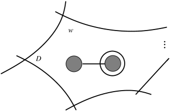
Figure 11. Nice type-$g$ stabilization in the domain $D$. The two full circles indicate the feet of the 1-handle we add to $\Sigma$, the contour of one of which is parallel to the new $\alpha$–curve, while the interval joining the two disks (which becomes a circle when completed in the 1-handle) is the new $\beta$–curve.

The expression “nice stabilization” will refer to either of the above types.

Remark 3.7.

The two types of nice stabilizations can be regarded as taking the connected sum of the multi-pointed Heegaard diagram $\mathfrak{D}$ with the diagrams (a) (for type-$b$ stabilization) and (b) (for type-$g$ stabilization) of Figure 12, depicting two diagrams for $S^{3}$. Since we take the connected sum in a domain $D$ containing a basepoint $w$, one of the basepoints of Figure 12 ($w_{2}$ for (a) and $w$ for (b)) should be eliminated.

\begin{picture}(9224.0,3458.0)(3025.0,-5081.0)\end{picture}

Figure 12. Two Heegaard diagrams of $S^{3}$. The left diagram is a spherical Heegaard diagram for $S^{3}$, with a single $\alpha$– and a single $\beta$–curve and two basepoints. The diagram on the right is the standard toroidal Heegaard diagram of $S^{3}$ with one basepoint.

In the sequel a nice move will mean either a nice isotopy, a nice handle slide or a nice stabilization/destabilization. It is an elementary fact that the result of a nice move on a multi-pointed Heegaard diagram of a 3–manifold $Y$ is also a multi-pointed Heegaard diagram of $Y$.

Theorem 3.8.

Suppose that $\mathfrak{D}^{\prime}=(\Sigma,\mbox{\boldmath$\alpha$}^{\prime},\mbox{\boldmath$\beta$}^{\prime},\mathbf{w}^{\prime})$ is given by a nice move on the nice diagram $\mathfrak{D}=(\Sigma,\mbox{\boldmath$\alpha$},\mbox{\boldmath$\beta$},\mathbf{w})$. Then $(\Sigma,\mbox{\boldmath$\alpha$}^{\prime},\mbox{\boldmath$\beta$}^{\prime},\mathbf{w}^{\prime})$ is nice, in the sense of Definition 3.1.

Proof.

The result of a nice move is a multi-pointed Heegaard diagram, so we need to check only that $\mathfrak{D}^{\prime}$ is nice, i.e. if an elementary domain contains no basepoint then it is either a bigon or a rectangle.

Consider a nice isotopy first. For a domain disjoint from the nice arc $\gamma$, the shape of the domain remains intact. Similarly, if a domain does not contain $\gamma(0)$ or $\gamma(1)$ then $\gamma$ splits off bigons and/or rectangles, and (by our assumption) a component which is not bigon or rectangle, which must contain a basepoint. Finally our assumptions on the domains $D_{1}$ and $D_{f}$ ensure that the resulting diagram is nice.

Suppose now that we perform a nice handle slide of $\alpha_{1}$ over $\alpha_{2}$. First consider the diagram which is identical to the nice diagram $\mathfrak{D}$ we started with, except we replace $\alpha_{1}$ by a new curve $\alpha_{1}^{\prime}$ which is the connected sum of $\alpha_{1}$ with $\alpha_{2}$ along $\delta$. To get the diagram $\mathfrak{D}^{\prime}$ (which is the result of the handle slide), we need to add a small isotopic translate of $\alpha_{2}$ (still denoted by $\alpha_{2}$) to this diagram. The curves $\alpha_{1}^{\prime}$, $\alpha_{1}$, and $\alpha_{2}$ bound a pair-of-pants in the Heegaard surface. (Notice that $\alpha_{1}$ is not in the diagram $\mathfrak{D}^{\prime}$.) The diagram $\mathfrak{D}^{\prime}$ has a collection of elementary domains which are rectangles, supported in the region between $\alpha_{1}^{\prime}$ and $\alpha_{2}$. There are also two bigons $B_{u}$ and $B_{d}$ in the new diagram, which are contained in the rectangle containing (in the old diagram $\mathfrak{D}$) the arc $\delta$, cf. Figure 9. There is a natural one-to-one correspondence between all other elementary domains in the diagram before and after the handle slide. The domain $D_{1}$ in the original diagram $\mathfrak{D}$ acquires four additional corners in the new diagram; all other domains have the same combinatorial shape before and after the handle slide. Since $D_{1}$ contains a basepoint, the new diagram $\mathfrak{D}^{\prime}$ is nice as well. See Figure 9 for an illustration.

Finally, a nice type-$b$ stabilization introduces three new bigons (one of which is with the basepoint $w^{\prime}$) and changes $D$ only. Since $D$ contains a basepoint, the resulting diagram is obviously nice. A nice type-$g$ stabilization changes only the domain $D$, hence if we start with a nice diagram, the fact that $D$ contains a basepoint implies that the result will be nice, concluding the proof. ∎

4. Convenient diagrams

Suppose now that $(\Sigma,\mbox{\boldmath$\alpha$},\mbox{\boldmath$\beta$})$ is an essential pair-of-pants diagram of a 3–manifold $Y$ which contains no $S^{1}\times S^{2}$–summand. In the following we will give an algorithm which provides a nice diagram from $(\Sigma,\mbox{\boldmath$\alpha$},\mbox{\boldmath$\beta$})$. Any output of this algorithm will be called a convenient diagram. (The algorithm will require certain choices, and depending on these choices we will have $\alpha$–, $\beta$– and symmetric convenient diagrams.) The algorithm involves seven steps, which we spell out in detail below.

Algorithm 4.1.

The following algorithm provides a nice multi-pointed Heegaard diagram from an essential pair-of-pants diagram $(\Sigma,\mbox{\boldmath$\alpha$},\mbox{\boldmath$\beta$})$ of a 3–manifold which has no $S^{1}\times S^{2}$–summand.

Step 1  Apply an isotopy on $\beta$ to get the bigon–free model of $(\Sigma,\mbox{\boldmath$\alpha$},\mbox{\boldmath$\beta$})$. Recall that by Theorem 2.10 the resulting diagram is unique (up to homeomorphism). We will henceforth use the notation $(\Sigma,\mbox{\boldmath$\alpha$},\mbox{\boldmath$\beta$})$ to denote this bigon-free model.

Step 2  Choose one of the curve systems $\alpha$ or $\beta$. Depending on the choice here, the result of the algorithm will be called $\alpha$–convenient or $\beta$–convenient. To ease notation, we will assume that we chose the $\alpha$–curves; for the other choice the subsequent steps must be modified accordingly.

Step 3  Put one basepoint into the interior of each hexagon, and two into the interior of each octagon of $(\Sigma,\mbox{\boldmath$\alpha$},\mbox{\boldmath$\beta$})$. Notice that in this way in each component of $\Sigma-\mbox{\boldmath$\alpha$}$ (and of $\Sigma-\mbox{\boldmath$\beta$}$) there will be two basepoints.

Step 4  Consider a component $P$ of $\Sigma-\mbox{\boldmath$\alpha$}$. Denoting parallel $\beta$–curves in $P$ with a single interval, the resulting digaram (after a suitable diffeomorphism of $P$) is one of the diagrams shown in Figure 6, together with the two basepoints chosen above. In case (i) connect the two basepoints with an oriented arc $a_{P}$ which crosses each of the vertical $\beta$–arcs once and is disjoint from all other curves in $P$. (The orientation of $a_{P}$ can be chosen arbitrarily. As we will see, the resulting convenient diagram will depend on the chosen orientation of $a_{P}$. For an example, see Figure 13(a).) In case (iii) connect the two basepoints with an oriented arc $a_{P}$ which intersects the $\beta$–arcs indicated by one of the horizontal arcs of Figure 6(iii), and which is disjoint from the $\beta$–arcs corresponding to the other two horizontal arcs, cf. Figure 13(b). Notice that for the arc therefore we have three possible choices; so, when taking possible orientations into account, altogether we have six choices in this case for $a_{P}$.

Figure 13. Possible oriented arcs. The left diagram shows the only possible choice for $a_{P}$ with one of its possible orientatons. In the right we show the three possible arcs, with one of their possible orientations.

Now, for each component $P_{j}$ of $\Sigma-\mbox{\boldmath$\alpha$}$ containing hexagons we fix an oriented arc $a_{P_{j}}$ as above.

Step 5  Choose a similar set of oriented arcs $b_{Q_{i}}$ for the basepoints, now using the components $Q_{i}$ of $\Sigma-\mbox{\boldmath$\beta$}$.

Step 6  Add a new $\alpha$–curve in each pair-of-pants component of $\Sigma-\mbox{\boldmath$\alpha$}$ as indicated by the dashed curves of Figure 14.

Figure 14. Addition of the new curves separating the two basepoints in a pair-of-pants. The basepoints are denoted by $w$.

The bigons in Figures 14(i) and (iii) are placed in the hexagon pointed into by the chosen oriented arc $a_{P}$, and in (iii) the bigon rests on the $\beta$–curve which is intersected by $a_{P}$. Although in the situation depicted in (ii) we also have a number of choices, we do not record them by choosing an arc. Notice that adding a curve as shown in (ii) in a pair-of-pants containing an octagon, we cut it into a hexagon, an octagon, a rectangle and a bigon (and some further rectangles between the parallel $\beta$–curves indicated by a single arc in the diagram). The union of the set $\alpha$ with the chosen new curves (a collection of $5g(\Sigma)-5$ curves altogether) will be denoted by $\mbox{\boldmath$\alpha$}^{c}$.

Step 7  Consider now a component $Q$ of $\Sigma-\mbox{\boldmath$\beta$}$. The intersection of $Q$ with $\alpha$ still falls into the three categories shown by Figure 6 (after a suitable diffeomorphism has been applied). After adding the new $\alpha$–curves, the patterns slightly change. The diagrams might contain bigons, and, when disregarding the bigons, we will have diagrams only of the shape of (i) and (iii) of Figure 6 (since after disregarding bigons there is no elementary domain which is an octagon). For the components where $Q\cap\mbox{\boldmath$\alpha$}$ looked like (i) or (iii) choose the new $\beta$–curve dictated by the chosen arcs $b_{Q}$, while in those domains where $Q\cap\mbox{\boldmath$\alpha$}$ is of (ii) (and then $Q\cap\mbox{\boldmath$\alpha$}^{c}$, after disregarding the bigons, became (i) or (iii)) we make further choices of oriented arcs and add the new $\beta$–curves accordingly. We assume that the bigons in the diagrams are very narrow and almost reach the basepoints — this convention helps deciding the intersection patterns between the bigons and the newly chosen curves. Like before, the completion of $\beta$ with the above choices will be denoted by $\mbox{\boldmath$\beta$}^{c}$.

Definition 4.2.

The resulting multi-pointed diagram $\mathfrak{D}=(\Sigma,\mbox{\boldmath$\alpha$}^{c},\mbox{\boldmath$\beta$}^{c},\mathbf{w})$ with $|\mathbf{w}|=4g(\Sigma)-4$ and $|\mbox{\boldmath$\alpha$}^{c}|=|\mbox{\boldmath$\beta$}^{c}|=5g(\Sigma)-5$ will be called a convenient diagram; depending on the choice made in Step 2, we call the diagram $\alpha$– or $\beta$–convenient.

A simple variation of Algorithm 4.1 provides a symmetric convenient diagram as follows: skip Step 2, add only one basepoint to an octagon in Step 3 and then apply Steps 4–7 modified so that in the components of $\Sigma-\mbox{\boldmath$\alpha$}$ (and of $\Sigma-\mbox{\boldmath$\beta$}$) described by Figure 6(ii) no new curves are added. The number of basepoints and the number of curves in a symmetric convenient diagram therefore depend on the genus of the Heegaard surface and the number of octagons in the bigon–free model. An example of a symmetric convenient diagram with no hexagons was discussed (and was called adapted) in [8].

Proposition 4.3.

Any $\alpha$–convenient ($\beta$–convenient or symmetric convenient) Heegaard diagram is nice.

Proof.

We only need to check that after adding both the new $\alpha$– and $\beta$–curves we do not create any further $2n$–gons with $n>2$ than the ones containing the basepoints. It is obvious from the construction that all basepoints will be in different components, and any $\alpha$– (and similarly $\beta$–) component contains a basepoint.

When adding the new curve in the situation of Figure 14(i), we have two choices, as encoded by the orientation of the arc connecting the two basepoints, pointing towards the region where the bigon is created. (Notice that the boundary circles of a pair-of-pants in (i) are not symmetric: one of the components is distinguished by the property that it is intersected by the same $\beta$–arc twice.) We will label the corresponding oriented arc with (i). In the case of Figure 14(ii) there are four possibilities, according to which boundary the newly added circle is isotopic to (when the basepoints are disregaded) and from which side it places the bigon. Since the modification of (ii) does not affect any other elementary $2n$–gon with $n>2$ besides the octagon we started with, the choice here will be irrelevant as far as the combinatorics of the other domains go, and (as in the algorithm) we do not record the choices made. For the case of Figure 14(iii) there are six choices, also indicated by an oriented arc connecting the two basepoints. These oriented arcs will be decorated by (iii).

Now for a given hexagon we must choose from these possibilities for both the $\alpha$– and the $\beta$–curves. This amounts to examining the changes on a hexagon with two oriented arcs pointing to (or from) the basepoint in the middle of the hexagon. The two oriented arcs (one corresponding to the fact that the hexagon is in an $\alpha$-component, the other that it is in a $\beta$-component) intersect either neighbouring, or opposite sides of the hexagon, and either can be a type (i) or type (iii), and can point in or out. Figure 15 shows the modification of the hexagon in each case. By drawing all possibilities for the two oriented arcs (taking symmetries and identities into account, there are 10 of them), and picturing the result on a given hexagon in Figure 16, the proof of the proposition is complete.

Figure 15. Possible oriented arcs and the effect of adding a new curve in a hexagon, dictated by the oriented arc.

∎

Figure 16. The list of all the cases in the proof of Proposition 4.3. In (1), (2), (3), (7), (8) the oriented arcs intersect the top horizontal and the upper left interval, while in (4), (5), (6), (9), (10) the top and bottom horizontals. For out-pointing oriented arcs (i) and (iii) has the same effect. In (1) the two oriented arcs are both (i) and point in, in (2) the vertical points in and is (i), the other points out, in (3) both point out. In (4) both point in and are (i), in (5) the top one points in and is (i), the other one points out, while in (6) both point out. (7), (8), (9) and (10) are the modifications of (1), (2), (4) and (5) by replacing the type (i) oriented arc with the type (iii) having the same direction.

We will define the Heegaard Floer chain complexes (determining the stable Heegaard Floer invariants) using combinatorial properties of convenient diagrams. Since in Algorithm 4.1 there are a number of steps which involve choices (recall that the algorithm itself starts with the choice of an essential pair-of-pants diagram for $Y$), it will be crucial for us to relate the results of various choices. The relations will be discussed in the next section.

Remark 4.4.

There are further possible choices for the dashed curves to turn an essential pair-of-pants diagram into a nice one. For example, Figure 17 shows an alternate configuration instead of Figure 14(i). Although such variants will be used in our later arguments, in the definition of convenient diagrams we chose the curve given by Figure 14(i), since this choice led to the least number of possibilities to examine.

Figure 17. An alternate curve for Figure 14(i).

5. Convenient diagrams and nice moves

The aim of the present section is to show that convenient diagrams of a fixed 3–manifold can be connected by nice moves. In order to state the main theorem of the section, we need a definition.

Definition 5.1.

Suppose that $\mathfrak{D}_{1},\mathfrak{D}_{2}$ are given nice diagrams of a 3–manifold $Y$. We say that $\mathfrak{D}_{1}$ and $\mathfrak{D}_{2}$ are nicely connected if there is a sequence $(\mathfrak{D}^{(i)})_{i=1}^{n}$ of nice diagrams all presenting the same $3$–manifold $Y$ such that

• $\mathfrak{D}_{1}=\mathfrak{D}^{(1)}$ and $\mathfrak{D}_{2}=\mathfrak{D}^{(n)}$, and

• consecutive elements $\mathfrak{D}^{(i)}$ and $\mathfrak{D}^{(i+1)}$ of the sequence differ by a nice move.

It is a simple exercise to verify that being nicely connected is an equivalence relation among nice diagrams representing a fixed 3–manifold $Y$. With the above terminology in place, in this section we will show

Theorem 5.2.

Suppose that $Y$ is a given 3–manifold which contains no $S^{1}\times S^{2}$–summand. Suppose that $\mathfrak{D}_{i}$ $(i=1,2)$ are convenient diagrams derived from essential pair-of-pants diagrams for $Y$. Then $\mathfrak{D}_{1}$ and $\mathfrak{D}_{2}$ are nicely connected.

Remark 5.3.

Notice that the diagrams in the path $(\mathfrak{D}^{(i)})_{i=1}^{n}$ connecting the two given convenient diagrams $\mathfrak{D}_{1}$ and $\mathfrak{D}_{2}$ are all nice, but not necessarily convenient for $i\neq 1,n$.

5.1. Convenient diagrams corresponding to a fixed pair-of-pants diagram

In this subsection, we wish to show that any two convenient diagrams belonging to a fixed essential pair-of-pants diagram can be nicely connected. We start by relating the $\alpha$–, $\beta$– and symmetric convenient Heegaard diagrams corresponding to the same pair-of-pants diagram and the same choice of oriented arcs.

Proposition 5.4.

Suppose that $\mathfrak{D}_{1}$ is an $\alpha$–convenient Heegaard diagram. Let $\mathfrak{D}_{2}$ denote the symmetric convenient diagram corresponding to the same pair-of-pants diagram and the same choice of oriented arcs fixed in Steps 4 and 5 of Algorithm 4.1. Then $\mathfrak{D}_{1}$ and $\mathfrak{D}_{2}$ are nicely connected.

Proof.

Let us fix an octagon of the bigon–free pair-of-pants decomposition underlying the convenient diagrams. We only need to work in the respective $\alpha$– or $\beta$–pair-of-pants containing this fixed octagon. To visualize the octagon better (and to indicate that arcs correspond to potentially more than one parallel segments), now we use two parallel $\beta$– (or $\alpha$–) curves from the bunch intersecting the pair-of-pants. In Figure 18(a) we show an $\alpha$–pair-of-pants (that is, the circles are all $\alpha$–curves, the newly chosen one being dashed, while the intervals denote the $\beta$–components in this pair-of-pants, and the dotted lines correspond to the new $\beta$–curve). Figure 18(b) shows a possible configuration in the $\beta$–pair-of-pants containing the same octagon (again, the new $\alpha$–curve is dashed while the new $\beta$–curve is dotted). Now the sequence of nice isotopies and nice handle slides on both the $\alpha$– and the $\beta$–curves, as indicated by the diagrams of Figure 18 (showing the effect of the nice moves only in the $\alpha$–pair-of-pants), transforms the diagram into Figure 18(g). From here, a nice type-$b$ destabilization (for each octagon) provides a symmetric convenient diagram (depicted by Figure 18(h)).

Figure 18. Isotopies and handle slides for showing that $\alpha$–convenient and symmetric convenient diagrams are nicely connected. Diagram (b) shows the $\beta$–pair-of-pants in the starting Heegaard diagram, all other diagrams are depicting the $\alpha$–pair-of-pants. Nice moves are indicated between consecutive diagrams. The new $\alpha$–curve appear as dashed, while the new $\beta$–curve as dotted segment(s).

∎

In view of the above result, when studying which diagrams can be nicely connected, it is no longer necessary to specify if a diagram is $\alpha$–convenient, $\beta$–convenient or symmetric. So we will typically drop this quantifier from the notation, and refer simply to convenient diagrams.

Next we will analyze the connection between convenient diagrams corresponding to a fixed pair-of-pants decomposition of $Y$.

Theorem 5.5.

Suppose that two convenient Heegaard diagrams $\mathfrak{D}_{1}$ and $\mathfrak{D}_{2}$ are derived from the same essential pair-of-pants diagram of a 3–manifold $Y$ which contains no $S^{1}\times S^{2}$–summand. Then the convenient diagrams are nicely connected.

Proof.

According to Proposition 5.4, we need to relate symmetric convenient Heegaard diagrams only. According to Algorithm 4.1, the two symmetric diagrams differ by the different choices of the oriented arcs connecting the basepoints sharing the same ($\alpha$– or $\beta$–) pair-of-pants components. Since the choice of these arcs is independent from each other, we only need to examine the case of changing one choice in one single pair-of-pants. The proof will rely on giving the sequence of diagrams, differing by nice moves, connecting the two different choices. Since we can work locally in a single pair-of-pants, these diagrams will not be very complicated. To simplify matters even more, we will follow the convention that bigons are omitted from the diagrams. Once again, we always imagine that bigons are very thin and almost reach the basepoint which is in the domain. Since nice moves cannot cross basepoints, the addition of these bigons will still keep niceness.

For the case of Figure 14(i) we need to specify only the direction of the oriented arc. As Figure 19 shows, the two choices can be connected by a nice handle slide and a nice isotopy.

Figure 19. Connecting different choices by nice moves for the configuration in Figure 14(i). In this case the difference between the chosen oriented arcs $a_{P}$ and $a^{\prime}_{P}$ providing the upper diagrams is in their orientations.

In the case depicted by Figure 14(iii) we need to consider the change of the oriented arc and the change of its direction. We can deal with the two cases separately; and as Figures 20 and 21 show, these changes can be achieved by nice isotopies and nice handle slides.

Figure 20. Connecting different choices by nice moves for the configuration in Figure 14(iii).The upper diagrams correspond to choosing the two arcs $a_{P}$ and $a_{P}^{\prime}$ in such a way that they intersect different horizontal arcs of Figure 6(iii).

Figure 21. Connecting different choices by nice moves for the configuration in Figure 14(iii). The two upper diagrams correspond to the choice of the same arc $a_{P}$ equipped with the two possible orientations.

∎

Remark 5.6.

Although it is not needed in the present situation, we will refer later to the simple fact that the choices given by Figure 14(i) and the one shown by Figure 17 are nicely connected.

5.2. Convenient diagrams corresponding to a fixed Heegaard decomposition

The next step in proving Theorem 5.2 is to relate convenient Heegaard diagrams which are derived from the same Heegaard decomposition but not necessarily from the same essential pair-of-pants Heegaard diagram. This is the most demanding part of the proof of Theorem 5.2, since now we need to work in the four-punctured sphere as opposed to the three-punctured sphere (as in Subsection 5.1).

Theorem 5.7.

Suppose that ${\mathcal{U}}$ is a fixed Heegaard decomposition of the 3–manifold $Y$, which contains no $S^{1}\times S^{2}$–summand. If $\mathfrak{D}_{i}$ are convenient diagrams of $Y$ derived from the essential pair-of-pants diagrams $(\Sigma,\mbox{\boldmath$\alpha$}_{i},\mbox{\boldmath$\beta$}_{i})$ $(i=1,2)$ both corresponding to ${\mathcal{U}}$, then $\mathfrak{D}_{1}$ and $\mathfrak{D}_{2}$ are nicely connected.

According to Lemma 2.6 (which rests on Theorem 2.3) two essential pair-of-pants diagrams determining the same Heegaard decomposition can be connected by a sequence of essential pair-of-pants diagrams, where the consecutive terms differ by a flip of one of the curve systems.

Thus, we need to connect two $\beta$–convenient diagrams which are derived from pair-of-pants decompositions $(\Sigma,\mbox{\boldmath$\alpha$},\mbox{\boldmath$\beta$})$ and $(\Sigma,\mbox{\boldmath$\alpha$}^{\prime},\mbox{\boldmath$\beta$})$, so that $\mbox{\boldmath$\alpha$},\mbox{\boldmath$\alpha$}^{\prime}$ and $\beta$ are markings, and $\mbox{\boldmath$\alpha$}^{\prime}$ is given by applying a flip to one of the curves in $\alpha$. Let $S$ denote the 4–punctured sphere in which the flip takes place, i.e. $S$ is the union of two pair-of-pants components of $\Sigma-\mbox{\boldmath$\alpha$}$. According to Theorem 5.5 we can assume that away from $S$ (i.e. for all basepoint pairs outside of $S$) and for all $\beta$–pair-of-pants we apply the same choices for the two convenient diagrams. Hence all differences between the convenient diagrams are localized in $S$.

First we would like to enumerate the possible configurations the $\beta$–curves can have in $S$. Let us first consider only those $\alpha$– and $\beta$–curves which were in the given pair-of-pants decomposition. We will denote these sets of elements still by $\alpha$ and $\beta$. Let $\mbox{\boldmath$\alpha$}_{1}$ denote $\mbox{\boldmath$\alpha$}-\{\alpha_{0}\}$, where $\alpha_{0}$ is the curve on which we will perform the flip. Recall that the curves in $\alpha$ and $\beta$ provide a bigon–free Heegaard diagram, hence by Proposition 2.14 the domains in $\Sigma-\mbox{\boldmath$\alpha$}_{1}-\mbox{\boldmath$\beta$}$ are either rectangles, hexagons or octagons. Recall also that further $\beta$–curves (and then $\alpha$–curves) are added to the diagram to turn it into a convenient diagram. By our previous discussion in Section 4, it follows that when forgetting about the bigons in $S$, the additional $\beta$–curves will cut the octagons into hexagons. (Once again, in our diagrams and considerations we will disregard the bigons. Since those can be assume to be very thin and almost reach the basepoints, the nice moves will remain nice even when adding these bigons back.) Assume now that we did add the new $\beta$–curves, but we did not add the new $\alpha$–curves in $S$ yet. (Recall that we are considering here a $\beta$–convenient diagram.) According to the above, we can assume that the domains of $S-\mbox{\boldmath$\beta$}$ are all hexagons. We continue to follow the convention that parallel $\beta$–arcs in $S$ are denoted by a single arc. The two pair-of-pants components contain four basepoints altogether, hence there are four hexagons in $S$. This means that there are six arcs partitioning $S$ into the four hexagons.

Lemma 5.8.

There are six possible configurations of six arcs to partition $S$ into four hexagons. These configurations are given by Figure 22 and are indexed by the four–tuples of degrees of the four boundary circles of $S$. (The degree of a circle is the number of arcs intersecting the circle.)

Figure 22. Possible configurations of $\beta$–curves in the 4–punctured sphere component of $\Sigma-\mbox{\boldmath$\alpha$}_{1}$. Boundary circles are all $\alpha$–curves, while the arcs are (parallel) $\beta$–curves in the 4–punctured sphere. As usual, we do not indicate the bigons and the basepoints.

Proof.

By contracting the boundary circles of $S$ to points, the above problem becomes equivalent to the enumeration of connected spherical graphs on four vertices involving six edges, such that no homotopically trivial and parallel edges are allowed. We can further partition the problem according to the number of loops (i.e. edges starting and arriving to the same vertex) the graph contains. Since we view the graphs on $S^{2}$, a loop partitions the remaining three points into a group of two and a single one. By connectedness the single one must be connected to the base of the loop. If there is no loop in the graph, then a simple combinatorial argument shows that the graph is a square with a diagonal, and with a further edge, for which we have two possibilities, corresponding to the graphs $(3,3,3,3)$ and $(4,4,2,2)$ of Figure 23, giving the corresponding configurations of Figure 22.

Figure 23. The six connected spherical graphs.

If the graph has one loop, then the only possibility in given by the diagram with index $(6,3,2,1)$. For two loops there are two possibilities (according to whether the bases of the loops coincide or differ); these are the graphs $(8,2,1,1)$ and $(5,5,1,1)$ of Figure 23, corresponding to the configurations $(8,2,1,1)$ and $(5,5,1,1)$ of Figure 22. Finally there is one possibility containing three loops, resulting in $(9,1,1,1)$ of Figure 23, giving rise to the configuration $(9,1,1,1)$ of Figure 22. ∎

Now let us put $\alpha_{0}$ back into $S$. Our next goal is to normalize the curve $\alpha_{0}$ in $S$. Notice that we could find a diffeomorphic model of $S$ in which $\alpha_{0}$ is the standard curve partitioning $S$ into two pairs-of-pants. With this model, however, the configuration of the $\beta$–curves might be rather complicated. We decided to work with a model of $S$ where the $\beta$–curves are standard (as depicted by Figure 22) and in the following we will normalize $\alpha_{0}$ by nice moves. In our subsequent diagrams we will always choose a circle, which we will call “outer” and which we will draw as outermost in our planar pictures, and which corresponds to the highest degree vertex of the spherical graph encountered in the previous proof. (If this vertex is not unique, we pick one of the highest degree vertices.) The other three boundary circles will be referred to as “inner” circles. Consider the pair-of-pants from the two components of $S-\alpha_{0}$ which is disjoint from the outer circle and denote it by $P$. Since we use a model for $S$ that conveniently normalizes the $\beta$–arcs but not necessarily $\alpha_{0}$, $P$ is not necessarily embedded in the standard way into $S$ (as, for example the pairs-of-pants in Figure 1 embed into the 4–punctured sphere). By an appropriate homeomorphism $\phi$ on $P$, however, the $\beta$–curves in $P$ can be normalized as before: since there are no octagons in $S$, the result will look like one of the diagrams of Figure 6(i) or (iii) (where $\alpha_{0}$ is the outer circle of $P$). The two cases will be considered separately. We start with the situation when the above pair-of-pants is of the shape of (i) (and call this Case A), and address the other possibility (Case B) afterwards. In the following we will show first that for any $\alpha_{0}$ there is a sequence of nice isotopies and handle slides which convert the curve system into one of finitely many cases which we will call “elementary curve configurations”.

Assume that we are in Case A. Consider the model of $P$ depicted by Figure 6(i) and connect the two boundary components of $P$ different from $\alpha_{0}$ by a straight line ${\tilde{a}}_{0}$, which therefore avoids the $\beta$–segments connecting different boundary components, and intersects the further segments (intersecting the outer boundary $\alpha_{0}$ of $P$ twice) transversely once each. In the model $\alpha_{0}$ can be given by considering the boundary of an $\epsilon$–neighbourhood (inside the model for $P$) of the union of ${\tilde{a}}_{0}$ with the two boundary circles it connects in $P$. Let $a_{0}$ denote the image of ${\tilde{a}}_{0}$ in $S$ (when identifying $P\subset S$ with the model of $P$ by the homeomorphism $\phi$). Consequently, $\alpha_{0}$ can be described by the arc $a_{0}$ connecting two boundary components of $S$: consider an $\epsilon$–neighbourhood of the union of $a_{0}$ together with the two boundary circles it connects. We can also assume that the arc $a_{0}$ passes through the two basepoints $w_{P}^{1}$ and $w_{P}^{2}$ contained by the pair-of-pants $P$, and we assume that these basepoints are near the boundary components of $P$ the arc $a_{0}$ connects. Fix the dual curve $a_{0}^{\prime}$ (connecting the other two boundary circles of $S$ in the complement of $a_{0}$, passing through the remaining two basepoints $w_{S-P}^{1}$ and $w_{S-P}^{2}$) and distinguish one of the basepoints from each pair outside and inside $P$, say $w_{P}^{2}$ and $w_{S-P}^{2}$. The latter will be denoted by $w_{d}$.

Our immediate aim is to show that the curve system under consideration can be transformed using nice moves into one of a finite collection of curve systems (or “elementary curve configurations”) described below. In order to state the precise result, first we need to consider oriented arc systems in the diagrams of Figure 22.

Definition 5.9.

Fix one of the diagrams of Figure 22, together with a distinguished basepoint $w_{d}$. An elementary situation is a collection of three disjoint oriented arcs $\gamma_{1}$, $\gamma_{2}$, and $\gamma_{3}$ in $S$ subject to the following constraints:

• each oriented arc $\gamma_{i}$ starts at one of the inner boundary circles, and there is only one arc starting at each inner circle,

• immediately after starting at an inner circle, each $\gamma_{i}$ passes through the basepoint of the domain (i.e. the $\gamma_{i}$ crosses this basepoint before crossing any of the other $\beta$-circles),

• the intersection of $\gamma_{i}$ with the $\beta$ is minimal in the following sense: there are no bigons in $S$ consisting of an arc in $\gamma_{i}$ and an arc in one of the $\beta$, and in fact, there are no triangles consisting of an arc in $\gamma_{i}$, an arc in $\beta$ and an arc in $\alpha_{i}$,

• each arc contains a unique basepoint, none of which is $w_{d}$, and finally

• each arc enters the domain of $w_{d}$ exactly once and points into it.

Before proceeding further, we give the list of all elementary situations.

Lemma 5.10.

Consider the configuration of $S$ depicted by $(3,3,3,3)$ of Figure 22, and fix $w_{d}$ in the lower left hexagon. Then there are four elementary situations of this case, given by Figure 24.

Figure 24. Elementary situations for (3,3,3,3) of Figure 22, with $w_{d}=w$ being chosen in the lower left hexagon.

Proof.

Consider the arc starting at the circle which is disjoint from the domain containing $w_{d}$. There are three choices for that arc (shown by (A), by (B) and (C), and by (D) of Figure 24), since after entering a domain (and passing through the basepoint there) the arc should enter and therefore stop at the domain of $w_{d}$. A similar simple case-by-case analysis for the remaining two arcs shows that Figure 24 lists all possibilities in this case. ∎

The further three possible choices of $w_{d}$ in the case of $(3,3,3,3)$ are all symmetric, hence (after possible rotations) the diagrams of Figure 24 provide a complete list of elementary situations in the case of $(3,3,3,3)$. Before listing all elementary situations for the remaining five possibilities of Figure 22 we make an observation. Suppose that $w_{d}$ is in a domain which has an inner circle on its boundary which circle is not adjacent to any other domain. (For example, in $(9,1,1,1)$ of Figure 22 there are three such domains.) Then there are no elementary situations with this choice of $w_{d}$, since $w_{d}$ could be the only basepoint for the arc starting at the inner circle, but that is not allowed by our definition. This observation cuts down the possible choices for the distinguished point $w_{d}$.

Lemma 5.11.

The elementary situations of the remaining five configurations of Figure 22 (up to symmetry) are shown by Figure 25.

Figure 25. Elementary situations for the further five possibilities of Figure 22.

Proof.

In $(9,1,1,1)$ there is only one domain into which we can place $w_{d}$ without having an empty set of elementary situations. For that choice the elementary situation is unique. For $(4,2,2,2)$ all four choices of domains for $w_{d}$ are possible and symmetric, for $(8,2,1,1)$ there are two (symmetric) choices. (Figure 25 shows only one of the symmetric choices.) For $(5,5,1,1)$ and $(6,3,2,1)$ there are two possible choices, the further choices are either symmetric, or do not provide any elementary situations. A fairly straightforward argument, similar to the one given in the proof of Lemma 5.10 now shows that Figure 25 provides all possible elementary situations. ∎

Now we return to the discussion of curve systems on the four–punctured sphere $S$. Notice first that an elementary situation provides a curve system on $S$: take each oriented arc, together with the boundary circle it starts from, and consider the boundary of an $\epsilon$–neighbourhood (for sufficiently small $\epsilon$) of it in $S$. The resulting curves, regarded as $\alpha$–curves (together with the basepoints on which the arcs passed through) provide a nice diagram on $S$ (which, together with curves on $\Sigma-S$, gives a nice diagram for $Y$). We will call these curve systems on $S$ elementary curve configurations.

Let us consider the curve $\alpha_{0}$ in $S$, which (according to our previous discussions) can be described by an arc $a_{0}$ connecting two boundary components of $S$. Recall first that in the $\beta$–convenient diagram there are further $\alpha$–curves: one in $P$ (separating the two basepoints on the arc $a_{0}$) and one in $S-P$ (separating the two basepoints on $a_{0}^{\prime}$). We choose these curves as follows.

Suppose first that $a_{0}$ enters and leaves the domain containing $w_{d}$ at least once. Then consider the subarc $a_{1}$ of $a_{0}$ which starts at one of its endpoints, passes through one of the basepoints and stops right before $a_{0}$ passes through the second basepoint, which we choose to be the distinguished one. The boundary of a small neighbourhood of the circle component from which $a_{1}$ starts and of $a_{1}$ now provides $\alpha_{1}$. In case $a_{0}$ does not enter and leave the domain of $w_{d}$ (for such a possibility see Figure 26(a)), we choose another curve $\alpha_{1}$: Instead of applying Figure 14(i), we rather apply the choice shown by Figure 17. In the above example the appropriate choice is given by Figure 26(b). A similar choice applied in the pair-of-pants $S-P$ gives $\alpha_{1}^{\prime}$; now the subarc $a_{1}^{\prime}$ will avoid the distinguished basepoint $w_{d}$. Now we are ready to state the result which nicely connects curve configurations in Case A to the elementary curve configurations.

Figure 26. A configuration when $a_{0}$ does not enter/leave the domain of $w_{d}$. In (b) the choice of $\alpha_{1}$ is shown.

Proposition 5.12.

Suppose that a $\beta$–convenient diagram $\mathfrak{D}_{1}$ in $S$ falling under Case A (with $\alpha_{0}$ given, and $\alpha_{1},\alpha_{1}^{\prime}$ chosen as above) is fixed. Then there is an elementary curve configuration $\mathfrak{D}_{2}$ such that $\mathfrak{D}_{1}$ and $\mathfrak{D}_{2}$ are nicely connected.

Proof.

First we will represent the three curves by three oriented arcs (which will resemble the presentation of elementary situations). We start by applying a nice handle slide on $\alpha_{0}$ over $\alpha_{1}$ performed at a segment of $\alpha_{0}$ neighbouring $w_{d}$. Notice that with the somewhat complicated choice of $\alpha_{1}$ given above, such a nice handle slide always exists: if the arc $a_{0}$ enters and leaves the domain of $w_{d}$ then the parallel portion of $\alpha_{0}$ and $\alpha_{1}$ provide the required (nice) handle slide, while in the other possibility for $a_{0}$, our modified choice of $\alpha_{1}$ makes sure of the existence of the handle slide. In Figure 27 we work out a particular example: (a) shows the two arcs $a_{0}$ and $a_{0}^{\prime}$ (the neighbourhoods of which, together with their endcircles, provide $\alpha_{0}$ and $\alpha_{0}^{\prime}$); the arc $a_{0}$ is solid, while $a_{0}^{\prime}$ is dashed on Fiure 27(a). Figure 27(b) shows $\alpha_{0}$ and $\alpha_{1}$, and also indicates the point where we take the handle slide; in this figure $\alpha_{0}$ is dashed and $\alpha_{1}$ is solid.

Figure 27. Simplifying the curves in an example to an elementary situation. In (a) the curve $a_{0}$ (solid) and $a_{0}^{\prime}$ (dashed) are shown, giving rise to $\alpha_{0}$ (dashed in (b)) and $\alpha_{0}^{\prime}$ (solid in (b)). Diagrams (c) and (d) show the points where the simplifications (by nice isotopies) should be performed. We pass from (e) to (f) by a nice isotopy again, and (f) is part of an elementary situation.

Perform the handle slide along a curve $\delta$ where $\delta(0)$ is the point of $\alpha_{0}$ in the domain $D_{w_{d}}$ of $w_{d}$ closest to $w_{d}$. To simplify notation, indicate $\alpha_{1}$ with the subarc defining it, with an arrow on its end which is not on a boundary component, and denote this oriented arc by $v_{1}$. The curve $a_{0}$, after the handle slide has been performed, will be indicated by a similar curve, this time however it starts at the other boundary component (which was connected to the first by $a_{0}$), passes through the other basepoint of $P$ and forks right before it reaches $v_{1}$. We put an arrow to both ends of the fork; the result will be denoted by $v_{0}$. The two curves in the chosen particular example are shown by Figure 27(c). A similar object is introduced for the last curve $\alpha_{0}^{\prime}$, which will be denoted by $v_{0}^{\prime}$ (and which, for simplicity, is not shown on Figure 27(c)). The result is reminiscent to the three oriented arcs in the definition of an elementary situation: we have three oriented ’arcs’ (one of which forks) starting at different inner circles, and passing through three basepoints of $S$ distinct from $w_{d}$. The arcs typically enter the domain containing $w_{d}$ many times. The curves $\alpha_{1},\alpha_{1}^{\prime}$ and $\alpha_{0}$ can be recovered from these arcs as the boundaries of the small neighbourhoods of the arcs together with the boundary circles the arcs start from.

Consider a point $p$ on one of the arcs which is in the domain $D_{w_{d}}$ containing $w_{d}$, which point $p$ can be connected to $w_{d}$ in the complement of all the oriented arcs within $D_{w_{d}}$, and when traversing on the arc containing $p$ to its end with an arrow, we leave $D_{w_{d}}$ at least once; see Figure 27(c) for such a point $p$. (If there is no such point on a certain arc, then the arc at question enters $D_{w_{d}}$ and immediately stops, exactly as arcs in an elementary situation do.) Now consider the same three arcs (one of which still might fork), and modify the one containing $p$ by terminating it at $p$. Consider the curve system corresponding to this modified set of oriented arcs. (The result of $v_{1}$ of our example under this operation is shown by Figure 27(d).) The rest of the arc (pointing from $p$ to the endpoint of the arc) then can be regarded as a curve $\gamma$ defininig an isotopy from this newly defined curve system back to the previous one. Since an arc can terminate either in $D_{w_{d}}$ next to $w_{d}$, or in the bigon defined by the fork, the isotopy defined by this $\gamma$ is a nice isotopy. Repeat this procedure as long as appropriate $p$ can be found (Figure 27(d) shows a further choice). The two arrows of the fork, together with an arc of the boundary of $D_{w_{d}}$, define a bigon. If there are no other arcs in this bigon, then, as above, the inverse of a nice isotopy can be used to eliminate the fork and replace it with a single oriented arc. (This is exactly what happens in Figure 27(e), and after applying this move, we get Figure 27(f), which is an elementary situation — at least it provides two curves of an elementary situation, and the third can be recovered easily from the above sequence of diagrams.)

By repeating the above procedure, we will get a collection of three disjoint oriented arcs, starting on the three inner circles and entering $D_{w_{d}}$ exactly once, hence we get an elementary situation. Since all the isotopies performed above are nice isotopies (or their inverses), the claim of the theorem follows at once. ∎

Before proceeding further with the proof of Theorem 5.4, let us describe our current position. We classified all possible background configurations of the $\beta$-curves in the four-punctured sphere where the flip on the $\alpha$-curves takes place (there are six types of these backgrounds). Then we divided the possible $\alpha$-curves into two classes (Case A and Case B), and showed that there is a finite number of possibilities for the $\alpha$-curves for each background (coming from the elementary situations) with which all other Case A configurations are nicely connected. What is left is to show that the Case B configurations and the elementary curve configurations (corresponding to a fixed background) are also nicely connected.

We proceed next to the classification of Case B configurations. Notice that (as for the Case A configurations) the curve $\alpha_{0}\subset S$ can be indicated by an arc $a_{0}$ connecting two inner boundary circles of $S$. (Then $\alpha_{0}$ is the boundary of the tubular neighbourhood in $S$ of this arc, together with the two boundary circles it connects.) The corresponding pair-of-pants is of the shape given by Figure 6(iii) exactly in case the arc $a_{0}$ defining $\alpha_{0}$ can be isotoped to be disjoint from all the $\beta$-arcs in $S$. This means that $a_{0}$ can be chosen to be parallel with one of the $\beta$-arcs in $S$. By fixing the outer circle, therefore for $(3,3,3,3)$ there are three Case B configurations, while this number is zero for $(9,1,1,1)$, $(8,2,1,1)$ and $(6,3,2,1)$, one for $(5,5,1,1)$ and two for $(4,4,2,2)$. Recall also that in Case A we distinguished a basepoint (called $w_{d}$) which is in a domain neighbouring the outer circle. We say that a Case B configuration is compatible with the choice of $w_{d}$ if the arc $a_{0}$ is not parallel to a boundary arc of the domain of $w_{d}$.

Now we are ready to show that all elementary curve configurations of Case A corresponding to a fixed background configuration of Figure 22 and a fixed distinguished point $w_{d}$, and all Case B configurations compatible with $w_{d}$ (and also correspond to the same background) are equivalent under nice handle slides and isotopies. As before, we give the arguments in detail for the case of $(3,3,3,3)$ as a background configuration, and then indicate the necessary modifications to be made for the other cases.

Proposition 5.13.

Fix a distinguished basepoint $w_{d}$ as before and consider all the elementary situations for the background $(3,3,3,3)$ with $w_{d}$ as the distinguished basepoint. Consider also the two Case B configurations compatible with the chosen $w_{d}$. The convenient diagrams corresponding to these choices are nicely connected.

Proof.

Consider the diagrams (1), (2) and (3) of Figure 28. The first two diagrams show the two Case B configurations (with the distinguished basepoint $w=w_{d}$), while the third diagram shows a Case A configuration which will be helpful in the proof.

Consider now the two placements of $\alpha_{1}$ (corresponding to the position of $\alpha_{0}$ given by Figure 28(1)) as shown by Figures 28(4) and (5). Since these two choices are two cases of adding a new curve in a pair-of-pants listed (iii) in Figure 6, Theorem 5.5 shows that the two choices give rise to nicely connected diagrams. On the other hand, by adding the last $\alpha$-curve as given by the dashed curve in (4) and (5), after a nice handle slide and nice isotopies we conclude that the elementary situations (A) and (B) of Figure 24 and the Case B configuration of (1) are nicely connected. The same two placements of $\alpha_{1}$ in the diagaram (2) (and the choice of $\alpha_{0}^{\prime}$ as shown in (C) or (D) of Figure 24) show that this Case B diagram is nicely connected with (C) and (D) of Figure 24. Putting the curve $\alpha_{1}$ into the diagram of (3) as given by Figures 28(6) and (7), a nice handle slide and nice isotopies turn this diagram into the elementary situations shown by (B) and (D) of Figure 24. In conclusion, we connected all the curve configurations corresponding to elementary situations (and also Case B configurations) with the distinguished basepoint $w=w_{d}$ by nice moves, concluding the proof of the proposition. ∎

Figure 28. Diagrams (4) and (5) connect (A) and (B) of Figure 24; here $w=w_{d}$. Similar choices in (2) and (3) connect (C) to (D) and (B) to (D) of Figure 24. Notice also that (1) and (2) give all Case B configurations compatible with the choice $w=w_{d}$.

Proposition 5.14.

Suppose that the $\beta$-curves are positioned in the four-punctured sphere $S$ as shown by $(3,3,3,3)$. Then all configurations are nicely connected.

Proof.

Since each Case B configuration is compatible with two choices of the distinguished basepoint, we can use these configurations to connect configurations with different fixed distinguished basepoints. The same argument applies if we change the choice of the outer circle, concluding the argument. ∎

The same strategy applies for the further five remaining backgrounds listed in Figure 22:

Theorem 5.15.

Consider a background configuration of Figure 22. Then the Case A elementary curve configurations and the Case B elementary curve configurations (if any) corresponding to the chosen background are nicely connected.

Proof.

The idea of the proof is exactly the same as the proof of Propositions 5.13 and 5.14, therefore we only provide the $\alpha_{0}$-circles which should be used in the same spirit as used in the proofs of the above propositions. Indeed, the circles can be defined by the dashed arcs of Figure 29. In each case one needs to make a careful (but rather straightforward) choice of the last $\alpha$-curve in the diagram; this last choice will not be given explicitly here. Notice that for $(9,1,1,1)$ there is one possible nontrivial place for $w_{d}$ and in this case there is only one elementary situation (and no Case B configuration), hence we do not need to do anything further. For the remaining cases the diagrams of Figure 29 provide the appropriate dashed arcs (as usual, the curves are the boundaries of the neighbourhoods of the unions of the arcs and the two circles they connect). ∎

Figure 29. Diagrams instructing how to connect elementary curve configurations. The circle $\alpha_{0}$ is given by the boundary of the neighbourhood of the dashed arc together with the two circles it connects. The further curves should be added as it is shown in Figure 28; hence there are more than one possibilities for them. Applying straightforward handle slides and isotopies, the individual diagrams can be used to connect different elementary curve configurations and Case B curve configurations.

Proof of Theorem 5.7.

Suppose that the convenient diagram $\mathfrak{D}_{i}$ is derived from the essential pair-of-pants diagram $(\Sigma,\mbox{\boldmath$\alpha$}_{i},\mbox{\boldmath$\beta$}_{i})$ ($i=1,2$). According to the assumption of the theorem, the two essential pair-of-pants diagrams represent the same Heegaard decomposition, therefore by Lemma 2.6 they are connected by a sequence of flips. Therefore it is enough to check the theorem in the case when the markings $\mbox{\boldmath$\alpha$}_{1}$ and $\mbox{\boldmath$\alpha$}_{2}$ differ by a flip and $\mbox{\boldmath$\beta$}_{1}=\mbox{\boldmath$\beta$}_{2}$. Suppose that the flip takes place in the four-punctured sphere $S\subset\Sigma$. The $\beta$–curves provide one of the configurations of Figure 22. According to Proposition 5.12 then both the curve systems $\mbox{\boldmath$\alpha$}_{1}$ and $\mbox{\boldmath$\alpha$}_{2}$ (before and after the flip) are nicely connected to either an elementary curve configuration or a Case B curve configuration. Applying Theorem 5.15 we conclude that the original Heegaard diagrams are nicely connected, finishing the proof of the theorem. ∎

Remark 5.16.

Notice that (since we normalized the shape of $\alpha_{0}$ in $S$), the same proof applies for $g$-flip equivalent configurations, hence we can use Theorem 11.1 of the Appendix instead of Theorem 2.3.

5.3. Convenient diagrams and stabilization

Next we consider the relation between convenient diagrams and stabilizations. Suppose that $(\Sigma,\mbox{\boldmath$\alpha$},\mbox{\boldmath$\beta$})$ is a bigon–free essential pair-of-pants Heegaard diagram for the 3-manifold $Y$ which contains no $S^{1}\times S^{2}$-summand. Choose a crossing $x$ of an $\alpha$– and a $\beta$–curve (called $\alpha_{1}$ and $\beta_{1}$) which is on the boundary of a domain $D$ which is either a hexagon or an octagon. Let $(\Sigma^{\prime},\mbox{\boldmath$\alpha$}^{\prime},\mbox{\boldmath$\beta$}^{\prime})$ denote the pair-of-pants Heegaard diagram we get by the stabilization procedure described in Lemma 2.15. In the following, ${\mathfrak{D}}$ will denote a symmetric convenient diagram derived from $(\Sigma,\mbox{\boldmath$\alpha$},\mbox{\boldmath$\beta$})$, while ${\mathfrak{D}}^{\prime}$ will be a symmetric convenient diagram we get from $(\Sigma^{\prime},\mbox{\boldmath$\alpha$}^{\prime},\mbox{\boldmath$\beta$}^{\prime})$ by applying the following choices:

• For any pair-of-pants which is away from the stabilization we apply the same choices as for ${\mathfrak{D}}$.

• For part of of the diagram we get by stabilizing the annuli $A_{\alpha}$ and $A_{\beta}$, there are no further choices to make. This is because these regions contain only rectangles and octagons, and our goal is to construct a symmetric convenient diagrams.

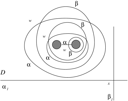
Figure 30. Stabilizations resuting the diagram $\mathfrak{D}_{1}$. The two full circles denote feet of a 1–handle. Basepoints are denoted by $w$.

Theorem 5.17.

The convenient diagrams ${\mathfrak{D}}$ and ${\mathfrak{D}}^{\prime}$ are nicely connected.

Proof.

Let us define the diagram $\mathfrak{D}_{1}$ by taking two nice type-$b$ and a nice type-$g$ stabilization in the elementary domain $D$ of $\mathfrak{D}$ containing a basepoint, where the pair-of-pants stabilization took place, as it is instructed by Figure 30. We would like to show that $\mathfrak{D}^{\prime}$ and $\mathfrak{D}_{1}$ can be connected by nice handle slides and nice isotopies.

Indeed, slide the $\alpha_{1}^{\prime\prime}$ (and similarly $\beta_{1}^{\prime\prime}$) of Figure 7 in $\mathfrak{D}^{\prime}$ over $\alpha_{1}$ (and $\beta_{1}$, resp.) by a nice handle slide, and apply nice isotopies until the resulting curves become part of the domain $D$. Repeat the same procedure now for the curves $\alpha_{1}^{\prime}$ and $\beta_{1}^{\prime}$. The resulting diagram is shown in Figure 31. Now it is easy to find a sequence of nice handle slides and nice isotopies connecting the diagram of Figure 31 and of Figure 30, concluding the proof of the theorem.

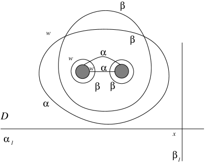
Figure 31. The diagram after the four nice handle slides and appropriate nice isotopies. Further nice handle slides and nice isotopies transform the diagram into Figure 30.

∎

Proof of Theorem 5.2.

Suppose that $(\Sigma_{i},\mbox{\boldmath$\alpha$}_{i},\mbox{\boldmath$\beta$}_{i})$ are essential pair-of-pants diagrams (corresponding to Heegaard decompositions ${\mathcal{U}}_{i}$) giving rise to convenient Heegaard diagrams $\mathfrak{D}_{i}$ ($i=1,2$). According to the Reidemesiter–Singer Theorem [21, 25] (see also [24]), the Heegaard decompositions ${\mathcal{U}}_{1}$ and ${\mathcal{U}}_{2}$ admit isotopic stabilizations. Let $(\Sigma,\mbox{\boldmath$\alpha$}^{i},\mbox{\boldmath$\beta$}^{i})$ denote the essential pair-of-pants diagram compatibe with the common Heegaard decomposition ${\mathcal{U}}$ we get by stabilizing the essential pair-of-pants diagram $(\Sigma_{i},\mbox{\boldmath$\alpha$}_{i},\mbox{\boldmath$\beta$}_{i})$. Choose a convenient diagram $\mathfrak{D}^{i}$ derived from $(\Sigma,\mbox{\boldmath$\alpha$}^{i},\mbox{\boldmath$\beta$}^{i})$. According to Theorem 5.17, the convenient diagrams $\mathfrak{D}_{i}$ and $\mathfrak{D}^{i}$ are nicely connected for $i=1,2$. On the other hand, $\mathfrak{D}^{1}$ and $\mathfrak{D}^{2}$ are now convenient diagrams corresponding to the same Heegaard decomposition, hence by Theorem 5.7 these diagrams are nicely connected. Since being nicely connected is transitive, the above argument shows that the convenient diagrams $\mathfrak{D}_{1}$ and $\mathfrak{D}_{2}$ are nicely connected, concluding the proof. ∎

6. The chain complex associated to a nice diagram

In this section we define the chain complex $({\widetilde{\rm{CF}}}(\mathfrak{D}),{\widetilde{\partial}}_{\mathfrak{D}})$ on which the definition of the stable Heegaard Floer invariant will rely. The definition of this chain complex is modeled on the definition of the Heegaard Floer homology groups ${\widehat{\rm{CF}}}$ of [12, 13], cf. also [23] and Section 10 of the present paper. In the next two sections we will deal with nice diagrams, and put our results concerning convenient diagrams temporarily aside.

Suppose that $\mathfrak{D}=(\Sigma=\Sigma_{g},\mbox{\boldmath$\alpha$}=\{\alpha_{i}\}_{i=1}^{k},\mbox{\boldmath$\beta$}=\{\beta_{j}\}_{j=1}^{k},\mathbf{w}=\{w_{1},\ldots,w_{k-g+1}\})$ is a nice multi-pointed Heegaard diagram for $Y$. An unordered $k$–tuple of points $\mathbf{x}=\{x_{1},\ldots,x_{k}\}\subset\Sigma$ will be called a generator if the intersection of $\mathbf{x}$ with any $\alpha$– or $\beta$–curve is exactly one point. In other words, $\mathbf{x}$ contains a unique coordinate from each $\alpha_{i}$ and from each $\beta_{j}$. Let $\mathcal{S}$ denote the set of these generators, and let

$${\widetilde{\rm{CF}}}(\mathfrak{D})=\oplus_{\mathbf{x}\in\mathcal{S}}\mathbb{F}$$

be the $\mathbb{F}$–vector space generated by the elements of ${\mathcal{S}}$. We will typically not distinguish an element of ${\mathcal{S}}$ from its corresponding basis vector in ${\widetilde{\rm{CF}}}(\mathfrak{D})$.

Definition 6.1.

(Cf. [23, Definition 3.2]) Fix two generators $\mathbf{x}$ and $\mathbf{y}\in\mathcal{S}$. We say that a 2n–gon from $\mathbf{x}$ to $\mathbf{y}$ is a formal linear combination $D=\sum n_{i}D_{i}$ of the elementary domains $D_{i}$ of $\mathfrak{D}=(\Sigma,\mbox{\boldmath$\alpha$},\mbox{\boldmath$\beta$})$, satisfying the following conditions:

• $x_{i}=y_{i}$ with $n$ exceptions;

• all multiplicities $n_{i}$ in $D$ are either 0 or 1, and at every coordinate $x_{i}\in\mathbf{x}$ (and similarly for $y_{i}\in\mathbf{y}$) either all four domains meeting at $x_{i}$ have multiplicity 0 (in which case $x_{i}=y_{i}$) or exactly one domain has multiplicity 1 and all three others have multiplicity 0 (when $x_{i}\neq y_{i}$);

• the support $s(D)$ of $D$, which is the union of the closures ${\overline{D}}_{i}$ of the elementary domains which have $n_{i}=1$ in the formal linear combination $D=\sum_{i}n_{i}D_{i}$ is a subspace of $\Sigma$ which is homeomorphic to the closed disk, with $2n$ vertices on its boundary;

• the $n$ coordinates (say $x_{1},\ldots,x_{n}$ and $y_{1},\ldots,y_{n}$) where $x_{i}$ differs from $y_{i}$ (which we call the moving coordinates) are on the boundary of $s(D)$ in an alternating fashion, in such a manner that, when using the boundary orientation of $s(D)$ (which is oriented by $\Sigma$) the $\alpha$–arcs point from $x_{i}$ to $y_{j}$ while the $\beta$–arcs from $y_{i}$ to $x_{j}$. In short, $\partial(\partial D\cap\mbox{\boldmath$\alpha$})=\mathbf{y}-\mathbf{x}$ and $\partial(\partial D\cap\mbox{\boldmath$\beta$})=\mathbf{x}-\mathbf{y}$.

The $2n$–gon is empty if the interior of $s(D)$ is disjoint from the basepoints $\mathbf{w}$ and the two given points $\mathbf{x}$ and $\mathbf{y}$. As before, for $n=1$ the $2n$–gon is called a bigon, while for $n=2$ it is a rectangle.

Notice that an empty bigon contains exactly one elementary bigon and some number of elementary rectangles, while an emtpy rectangle is the union of some number of elementary rectangles.

Suppose that $\mathbf{x},\mathbf{y}\in{\widetilde{\rm{CF}}}(\mathfrak{D})$ are two generators. Define the $\pmod{2}$ number $m_{\mathbf{x}\mathbf{y}}\in\mathbb{F}$ to be the cardinality $\pmod{2}$ of the set ${\mathfrak{M}}_{\mathbf{x},\mathbf{y}}$ defined as follows. We declare ${\mathfrak{M}}_{\mathbf{x},\mathbf{y}}$ to be empty if $\mathbf{x}$ and $\mathbf{y}$ are either equal or differ in at least three coordinates. If $\mathbf{x}$ and $\mathbf{y}$ differ at exactly one coordinate, then we define ${\mathfrak{M}}_{\mathbf{x},\mathbf{y}}$ as the set of empty bigons from $\mathbf{x}$ to $\mathbf{y}$, while if $\mathbf{x}$ and $\mathbf{y}$ differ in exactly two coordinates, then ${\mathfrak{M}}_{\mathbf{x},\mathbf{y}}$ is the set of empty rectangles from $\mathbf{x}$ to $\mathbf{y}$. It is easy to see that either ${\mathfrak{M}}_{\mathbf{x},\mathbf{y}}$ is empty or it contains one or two elements. The two elements of ${\mathfrak{M}}_{\mathbf{x},\mathbf{y}}$ can be distinguished by the part of the $\alpha$– (or $\beta$–) curves containing the moving coordinates that are in the boundary of the domain. (If $\mathbf{x}$ and $\mathbf{y}$ differ in exactly one coordinate and ${\mathfrak{M}}_{\mathbf{x},\mathbf{y}}$ contains two elements, then there are isotopic $\alpha$– and $\beta$–curves.)

Now define the boundary operator

$${\widetilde{\partial}}_{\mathfrak{D}}\colon{\widetilde{\rm{CF}}}(\mathfrak{D})\to{\widetilde{\rm{CF}}}(\mathfrak{D})$$

by the formula

$${\widetilde{\partial}}_{\mathfrak{D}}(\mathbf{x})=\sum_{\mathbf{y}\in\mathcal{S}}m_{\mathbf{x}\mathbf{y}}\cdot\mathbf{y}$$

on the generators, and extend the map linearly to ${\widetilde{\rm{CF}}}(\mathfrak{D})$.

For future reference, it will be convenient to have an alternative characterization of ${\widetilde{\partial}}_{\mathfrak{D}}$. To this end, it will help to generalize Definition 6.1 as follows:

Definition 6.2.

Suppose that $\mathbf{x},\mathbf{y}\in\mathcal{S}$ are two generators in the Heegaard diagram $(\Sigma,\mbox{\boldmath$\alpha$},\mbox{\boldmath$\beta$})$. A domain connecting $\mathbf{x}$ to $\mathbf{y}$ (or, when $\mathbf{x}$ and $\mathbf{y}$ are implicitly understood, simply a domain) is a formal linear combination $D=\sum_{i}n_{i}\cdot D_{i}$ of the elementary domains, which in turn can be thought of as a $2$-chain in $\Sigma$, satisfying the following constraints. Divide the boundary $\partial D$ of the 2-chain $D$ as $a+b$, where $a$ is supported in $\alpha$ and $b$ is supported in $\beta$. Then, thinking of $\mathbf{x}$ and $\mathbf{y}$ as 0-chains, we require that $\partial a=\mathbf{y}-\mathbf{x}$ (and hence $\partial b=\mathbf{x}-\mathbf{y}$). The set of domains from $\mathbf{x}$ to $\mathbf{y}$ will be denoted by $\pi_{2}(\mathbf{x},\mathbf{y})$.

Less formally, for each $i=1,\dots,g$, the portion of $\partial D$ in $\alpha_{i}$ determines a path from the $\alpha_{i}$–coordinate of $\mathbf{x}$ to the $\alpha_{i}$–coordinate of $\mathbf{y}$, and the portion of $\partial D$ on $\beta_{i}$ determines a path from the $\beta_{i}$–coordinate of $\mathbf{y}$ to the $\beta_{i}$–coordinate of $\mathbf{x}$.

Definition 6.3.

A domain $D=\sum n_{i}\cdot D_{i}$ is nonnegative (written $D\geq 0$) if all $n_{i}\geq 0$. Given an elementary domain $D_{i}$, the coefficient $n_{i}$ is called the multiplicity of $D_{i}$ in $D$. Equivalently, given a point $z\in\Sigma-\mbox{\boldmath$\alpha$}-\mbox{\boldmath$\beta$}$ the local multiplicity of $D$ at $z$, denoted $n_{z}(D)$, is the multiplicity of the elementary domain $D_{i}$ containing $z$ in $D$. For $\mathbf{w}=\{w_{1},\ldots,w_{k}\}$ we define $n_{\mathbf{w}}(D)=\sum_{i}n_{w_{i}}(D)$.

It is often fruitful to think of domains from the following elementary point of view. A domain $D$ connecting $\mathbf{x}$ to $\mathbf{y}$ is a linear combination of elementary domains whose local multiplicities satisfy a system of linear equations, one for each intersection point $p$ of $\alpha_{i}$ with $\beta_{j}$. To describe these relations, we need a little more notation. At each intersection point $p$ of $\alpha_{i}$ and $\beta_{j}$ there are four (not necessarily distinct) elementary domains, which we label clockwise as $A_{p}$, $B_{p}$, $C_{p}$, and $D_{p}$, so that $A_{p}$ and $B_{p}$ are above $\alpha_{i}$ and $B_{p}$ and $C_{p}$ are to the right of $\beta_{j}$, cf. Figure 32. Let $a_{p}$, $b_{p}$, $c_{p}$, and $d_{p}$ denote the multiplicities of $A_{p}$, $B_{p}$, $C_{p}$, and $D_{p}$ in $D$.

Figure 32. The quadrants $A_{p},B_{p},C_{p}$ and $D_{p}$ at a crossing.

For a generator $\mathbf{x}\in{\mathcal{S}}$ and an intersection point $q$ define

$$\delta(q,\mathbf{x})=\left\{\begin{array}[]{ll}+1&{\text{if $q\in\mathbf{x}$}}\\ 0&{\text{otherwise.}}\end{array}\right.$$

Lemma 6.4.

The formal linear combination $D=\sum D_{i}$ is in $\pi_{2}(\mathbf{x},\mathbf{y})$ (ie. is a domain from $\mathbf{x}$ to $\mathbf{y}$) if, for each $p\in\alpha_{i}\cap\beta_{j}$, we have that

$$a_{p}+c_{p}=b_{p}+d_{p}-\delta(p,\mathbf{x})+\delta(p,\mathbf{y}).$$ (6.1)

Proof.

Consider the quadrants around each intersection point $p$ as illustrated in Figure 32. The right horizontal arc (between $B_{p}$ and $C_{p}$, oriented out of $p$) appears in $\partial D$ with multiplicity $b_{p}-c_{p}$, while the left horizontal arc (between $A_{p}$ and $D_{p}$, oriented into $p$) appears in $\partial D$ with multiplicity $a_{p}-d_{p}$. Thus, the point $p$ appears in $\partial(\partial D\cap\alpha_{i})$ with multiplicity $a_{p}+c_{p}-b_{p}-d_{p}$; and in a domain from $\mathbf{x}$ to $\mathbf{y}$, each coordinate appears with multiplicity $\delta(p,\mathbf{y})-\delta(p,\mathbf{x})$. Equation (6.1) then follows. ∎

It is straightforward to see that if $D=\sum n_{i}D_{i}\in\pi_{2}(\mathbf{x},\mathbf{y})$ then $-D\in\pi_{2}(\mathbf{y},\mathbf{x})$, and for the sum $D+D^{\prime}$ with $D\in\pi_{2}(\mathbf{x},\mathbf{y})$ and $D^{\prime}\in\pi_{2}(\mathbf{y},\mathbf{z})$ we have $D+D^{\prime}\in\pi_{2}(\mathbf{x},\mathbf{z})$.

Suppose that $(\Sigma,\mbox{\boldmath$\alpha$},\mbox{\boldmath$\beta$},\mathbf{w})$ is a nice multi-pointed Heegaard diagram, and assume that the elementary domain $D_{i}$ is a $2n$–gon. Define $e(D_{i})$ by the formula $1-\frac{n}{2}$, and extend this definition linearly to all domains with $n_{w_{i}}=0$ ($i=1,\ldots,k-g+1$). The resulting quantity $e(D)$ is the Euler measure of $D$.

Remark 6.5.

The Euler measure has a natural interpretation in terms of the Gauss-Bonet theorem as follows. Endow $\Sigma$ with a metric for which all $\alpha_{i}$ and $\beta_{j}$ are geodesics, meeting at right angles. The Euler measure of an elementary domain is the integral of the curvature of this metric. Notice that this alternate definition applies for elementary domains which are not $2n$–gons.

If $D\in\pi_{2}(\mathbf{x},\mathbf{y})$, then for each $\mathbf{x}$– (and $\mathbf{y}$–) coordinate $x_{i}$ (and $y_{j}$) consider the average of the multiplicities of the four domains meeting at $x_{i}$ (and $y_{j}$). The sum of the resulting numbers $p_{x_{i}}(D)$ and $p_{y_{j}}(D)$ will be denoted by $p(D)$ and is called the point measure of $D$. We define the Maslov index $\mu(D)$ to be the sum

$$\mu(D)=e(D)+p(D).$$ (6.2)

Remark 6.6.

The term “Maslov index” is used here since, according to a theorem of Lipshitz [2], the quantity defined in Equation (6.2) computes the expected dimension of the moduli space of curves associated to the domain $D$.

It will be useful to have another construction; before introducing it, we pause for a definition:

Definition 6.7.

An elementary $\alpha$-arc $a$ is a subarc of $\alpha_{i}\subset\Sigma$ which connects two intersection points $x_{1}=\alpha_{i}\cap\beta_{j}$ and $x_{2}=\alpha_{i}\cap\beta_{k}$ such that int$(a)$ contains no further intersection points, ie. int$(a)\cap\mbox{\boldmath$\beta$}=\emptyset$. A similar definition gives the notion of elementary $\beta$–arcs. Let ${\mathcal{A}}$ denote the set of all elementary arcs ($\alpha$– or $\beta$–) of the diagram. It follows from the definition that an elementary arc $a$ is in the boundary of two (not necessarily distinct) elementary domains $D_{l}$ and $D_{r}$.

Let $\mathbf{x},\mathbf{y}\in\mathcal{S}$ be two generators and consider $D\in\pi_{2}(\mathbf{x},\mathbf{y})$ with $D\geq 0$. A topological space $S$, together with a tiling on it, and a map $f\colon S\to\Sigma$ can be built from $D$ in the following way. If an elementary domain $D_{i}$ appears in $D$ with multiplicity $n_{i}>0$ then take $n_{i}$ copies of $D_{i}$ and denote them by $D_{i}^{(1)},D_{i}^{(2)},\ldots,D_{i}^{(n_{i})}$. Suppose now that $a\subset\alpha_{t}$ is an $\alpha$–elementary arc in the boundary of the elementary domains $D_{i}$ and $D_{j}$, and assume without loss of generality that $n_{i}\leq n_{j}$. Then glue $D_{i}^{(1)}$ to $D_{j}^{(1)},D_{i}^{(2)}$ to $D_{j}^{(2)},\ldots,D_{i}^{(n_{i})}$ to $D_{j}^{(n_{i})}$ along the part of their boundary corresponding to the arc $a$. If $b\subset\beta_{l}$ is a $\beta$–elementary arc on the boundary of $D_{i}$ and $D_{j}$ (and once again $n_{i}\leq n_{j}$), then glue $D_{i}^{(n_{i})}$ to $D_{j}^{(n_{j})},D_{i}^{(n_{i}-1)}$ to $D_{j}^{(n_{j}-1)},\ldots,D_{i}^{(1)}$ to $D_{j}^{(n_{j}-n_{i}+1)}$ along the part of their boundary corresponding to the arc $b$. The existence of both the tiling and the contiuous map $f$ obviously follow from the construction. (Note that this construction is similar to the construction of the surface in [2]: the only difference is the manner in which we handle the corner points.)

Proposition 6.8.

Suppose that for the domain $D\in\pi_{2}(\mathbf{x},\mathbf{y})$ we have $D\geq 0$, $n_{\mathbf{w}}(D)=0$ and suppose that at each coordinate $x_{i}\in\mathbf{x}$ and $y_{j}\in\mathbf{y}$, we have that $p_{x_{i}}(D)$ and $p_{y_{j}}(D)$ are strictly less than $1$. Then the topological space $S$ defined above is a surface with boundary and with corner points corresponding to the points $z\in\mathbf{x}\cup\mathbf{y}$ with $p_{z}(D)\equiv\frac{1}{4}\pmod{\frac{1}{2}}$.

Proof.

The above construction provides a smooth manifold-with-boundary over each point $t\in D$ which is not one of the coordinates of $\mathbf{x}$ or $\mathbf{y}$. At coordinates of $\mathbf{x}$ or $\mathbf{y}$, there are only a few ways the local multiplicities can distribute over the four adjoining regions. Indeed, up to cyclic orderings (reading clockwise around $t$) we can have one of the following distributions: $(1,0,0,0)$, $(1,1,0,0)$, $(1,2,0,0)$, $(2,1,0,0)$, and $(1,1,1,0)$. Following the above construction, we see that in all but the second case, the surface $S$ has a corner over $t$. ∎

Proposition 6.9.

Suppose that $\mathfrak{D}$ is a nice multi-pointed Heegaard diagram. Suppose furthermore that for $D\in\pi_{2}(\mathbf{x},\mathbf{y})$ we have $D\geq 0$, $n_{\mathbf{w}}(D)=0$ and $\mu(D)=1$. Then either

(a) $e(D)=\frac{1}{2}$ and the point measures $p_{x_{i}}(D)=p_{y_{i}}(D)$ vanish with a single exception $i=j$, for which both point measures $p_{x_{j}}(D)=p_{y_{j}}(D)$ are equal to $\frac{1}{4}$, or

(b) $e(D)=0$ and the point measures vanish with two exceptional indices $i,j$ for which $p_{x_{i}}(D)=p_{x_{j}}(D)=p_{y_{i}}(D)=p_{y_{j}}(D)=\frac{1}{4}$.

Proof.

Notice that since $D\geq 0$, by definition $p(D)$ is a positive multiple of $\frac{1}{4}$ and (since the Heegaard diagram is nice) the Euler measure $e(D)$ is a nonnegative multiple of $\frac{1}{2}$. Therefore the condition $\mu(D)=e(D)+p(D)=1$ implies that either

(a) $e(D)=\frac{1}{2}$ and $p(D)=\frac{1}{2}$ (implying $(p_{x_{1}}(D),p_{y_{1}}(D))=(\frac{1}{4},\frac{1}{4})$) or

(b) $e(D)=0$ and $p(D)=1$. In this latter case we have three possibilities for the point measures:

1. $(p_{x_{1}}(D),p_{x_{2}}(D),p_{y_{1}}(D),p_{y_{2}}(D))=(\frac{1}{4},\frac{1}{4},\frac{1}{4},\frac{1}{4})$ or

2. $(p_{x_{1}}(D),p_{y_{1}}(D))=(\frac{1}{2},\frac{1}{2})$ or

3. $(p_{x_{1}}(D),p_{y_{1}}(D))=(\frac{3}{4},\frac{1}{4})$.

Case (a) is exactly the first and (1) of Case (b) is the second possibility given by the proposition. We claim that (2) and (3) of Case (b) cannot exist. When the point measure $(p_{x_{1}}(D),p_{y_{1}}(D))$ is equal to $(\frac{1}{2},\frac{1}{2})$, we have that the two points $x_{1}$ and $y_{1}$ are equal and the entire $\alpha$– (or $\beta$–) circle containing it is in the boundary $\partial D$. Since the domain is in one of its side, by Lemma 3.2 we conclude that $n_{\mathbf{w}}(D)\neq 0$, a contradiction.

Finally, we need to exclude the possibility for the point measures to be equal to $(p_{x_{1}}(D),p_{y_{1}}(D))=(\frac{3}{4},\frac{1}{4})$. This can in principle happen in one of two ways: either all local multiplicities around the corner point with multiplicity $\frac{3}{4}$ are bounded above by one, or not. In the latter case, there is some curve, say $\alpha_{i}$ (or $\beta_{j}$, but that is handled in exactly the same manner) with the property that the local multipicities of $D$ at the corner point are strictly greater on one side of $\alpha_{i}$ than they are on the other. From this, it follows globally that the local multiplicities of $D$ are strictly greater on one side of $\alpha_{i}$ than they are on the other. Since $D$ is a nonnegative domain, it follows that $D$ contains all the elementary domains on one side of $\alpha_{i}$. In view of Lemma 3.2, this violates the condition that $n_{\mathbf{w}}(D)=0$. We return now to the case where all local multiplicities are $\leq 1$. In this case, Proposition 6.8 constructs a surface $S$ mapping to $D$. It is easy to see that $S$ has a single boundary component, and hence its Euler characteristic is congruent to $1\pmod{2}$. Note that $S$ is an unbranched cover of a subsurface of $\Sigma$, and hence its Euler measure is calculated as the Euler measure of $D$. On the other hand, by the Gauss-Bonet theorem, the Euler measure of $S$ coincides with its Euler characteristic (since the correction terms coming from the two corners cancel). But the Euler measure $e(D)$ is zero, contradicting $\chi(S)\equiv 1$ (mod 2). ∎

We now give the following result essentially from [23, Theorem 3.3], where it is shown that the Maslov index one pseudo-holomorphic disks in a nice diagram are (empty) embedded bigons and rectangles. The proof of this result consists of two parts. In the first, it is shown that the properties of the index formula ensure that the holomorphic curves that need to be counted correspond to bigons and rectangles mapping into $\Sigma$. The second, combinatorial part, shows that such bigons and rectangles are in fact embedded.

The version we need here is slightly different. It states that the index one (as defined by Equation (6.2)) nonnegative domains are embedded bigons and rectangles. Again, the argument can be thought of as consisting of two parts. In the first part, it is shown that a nonnegative, index one domain corresponds to an immersed bigon or rectangle (this is, effectively, Proposition 6.9 above). Once this is done, the proof that the corresponding domain is in fact an embedded bigon or rectangle proceeds exactly as in [23].

Proposition 6.10.

The space ${\mathfrak{M}}_{\mathbf{x},\mathbf{y}}$ of empty rectangles and bigons connecting $\mathbf{x}$ and $\mathbf{y}$ can be described by

$${\mathfrak{M}}_{\mathbf{x},\mathbf{y}}=\{D\in\pi_{2}(\mathbf{x},\mathbf{y})\mid D\geq 0,\ n_{\mathbf{w}}(D)=0,\ \mu(D)=1\}.$$

Proof.

For $D\in{\mathfrak{M}}_{\mathbf{x},\mathbf{y}}$ we have, by definition, that $D\in\pi_{2}(\mathbf{x},\mathbf{y})$ and $D\geq 0$ (since all coefficients are either 0 or 1). Since $D$ is empty, we have also $n_{\mathbf{w}}(D)=0$ and that all coordinates which do not move have vanishing point measure. In addition, the moving coordinates have point measure $\frac{1}{4}$. Now if $D$ is a bigon, then it contains a unique elementary bigon, hence its Euler measure is $\frac{1}{2}$, and since it has two moving coordinates $x_{i},y_{i}$, we conclude that $p(D)=\frac{1}{2}$, implying $\mu(D)=1$. If $D$ is a rectangle, then $e(D)=0$ and since there are four moving coordinates, we get $p(D)=1$, showing again that $\mu(D)=1$. Therefore $D\in{\mathfrak{M}}_{\mathbf{x},\mathbf{y}}$ satisfies the three required properties.

Assume conversely that $D\in\pi_{2}(\mathbf{x},\mathbf{y})$ satisfies $D\geq 0$, $n_{\mathbf{w}}(D)=0$ and $\mu(D)=1$. Notice first that these properties imply that $p(D)\leq 1$, hence, in particular, $D$ is empty, i.e. does not contain any coordinate $x_{i}$ (or $y_{i}$) in its interior. Consider now the surface-with-boundary $S$ with the map $f\colon S\to\Sigma$ representing $D$ and the tiling given on $S$, as constructed in Proposition 6.8. In view of Proposition 6.9, $S$ is a disk with either two or four corner points, each of which has $90^{\circ}$ angle. Now the same line of reasoning as the one given for [23, Theorem 3.3] shows that $f$ is an embedding and $D$ is a bigon or rectangle, hence $D\in{\mathfrak{M}}_{\mathbf{x},\mathbf{y}}$, concluding the proof. ∎

With the above identity, the boundary operator ${\widetilde{\partial}}_{\mathfrak{D}}$ can be rewritten on $\mathbf{x}\in\mathcal{S}$ as

$${\widetilde{\partial}}_{\mathfrak{D}}\mathbf{x}=\sum_{\mathbf{y}\in\mathcal{S}}\sum_{\{D\in\pi_{2}(\mathbf{x},\mathbf{y})\big{|}D\geq 0,n_{\mathbf{w}}(D)=0,\mu(D)=1\}}\mathbf{y}.$$

We now turn back to the study of the pair $({\widetilde{\rm{CF}}}(\mathfrak{D}),{\widetilde{\partial}}_{\mathfrak{D}})$.

Theorem 6.11.

The pair $({\widetilde{\rm{CF}}}(\mathfrak{D}),{\widetilde{\partial}}_{\mathfrak{D}})$ is a chain complex, that is, ${\widetilde{\partial}}_{\mathfrak{D}}^{2}=0$.

Proof.

We need to show that for any pair of generators $\mathbf{x},\mathbf{z}$ the matrix element

$$\langle{\widetilde{\partial}}_{\mathfrak{D}}^{2}\mathbf{x},\mathbf{z}\rangle$$

is zero (mod 2). Notice that the above matrix element is simply the cardinality of the set

$${\mathfrak{N}}_{\mathbf{x}\mathbf{z}}=\bigcup_{\mathbf{y}\in\mathcal{S}}{\mathfrak{M}}_{\mathbf{x},\mathbf{y}}\times{\mathfrak{M}}_{\mathbf{y},\mathbf{z}}.$$

The proof that ${\mathfrak{N}}={\mathfrak{N}}_{\mathbf{x}\mathbf{z}}$ contains an even number of elements will be partitioned into three subcases. Define

$${\mathfrak{N}}(b)=\{(D_{1},D_{2})\in{\mathfrak{N}}\mid{\mbox{both }}D_{i}{\mbox{ are bigons}}\}.$$

In a similar vein, define ${\mathfrak{N}}(r)$ as the set of pairs $(D_{1},D_{2})\in{\mathfrak{N}}$ when both $D_{i}$ are rectangles, and finally define the set of mixed pairs ${\mathfrak{N}}(m)$ consisting of those $(D_{1},D_{2})$ of ${\mathfrak{N}}$ in which one of the domains is a bigon and the other one is a rectangle. Obviously

$${\mathfrak{N}}={\mathfrak{N}}(b)\cup{\mathfrak{N}}(r)\cup{\mathfrak{N}}(m)$$

is a disjoint union, and if all the above subsets have even cardinality, the evenness of $|{\mathfrak{N}}|$ follows at once.

Case 1: Examination of ${\mathfrak{N}}(b)$. The set ${\mathfrak{N}}(b)$ will be further partitioned as follows: Suppose that $(D_{1},D_{2})\in{\mathfrak{N}}(b)$. Let $i$ (and $j$) denote the moving coordinate of $D_{1}$ (of $D_{2}$ resp.). Let ${\mathfrak{N}}(b)_{1}$ denote the set of pairs $(D_{1},D_{2})\in{\mathfrak{N}}(b)$ with $i=j$, and ${\mathfrak{N}}(b)_{2}$ the set of those pairs where $i\neq j$.

Suppose that the pair of bigons $(D_{1},D_{2})\in{\mathfrak{M}}_{\mathbf{x},\mathbf{y}}\times{\mathfrak{M}}_{\mathbf{y},\mathbf{z}}$ for some $\mathbf{y}\in\mathcal{S}$ is in ${\mathfrak{N}}(b)_{2}$. Since the moving coordinate of $D_{1}$ is $i$, we get that $x_{j}=y_{j}$, therefore the bigon $D_{2}\in{\mathfrak{M}}_{\mathbf{y},\mathbf{z}}$ can be regarded as a bigon $D_{1}^{\prime}=D_{2}\in{\mathfrak{M}}_{\mathbf{x},\mathbf{y}^{\prime}}$, where the coordinates of $\mathbf{y}^{\prime}$ are given as $y_{k}^{\prime}=x_{k}(=z_{k})$ for all $k\neq i,j$, $y_{i}^{\prime}=x_{i}$ and $y_{j}^{\prime}=z_{j}$. With this choice of $\mathbf{y}^{\prime}$ it is easy to see that $D_{2}^{\prime}=D_{1}$ can be regarded as an element of ${\mathfrak{M}}_{\mathbf{y}^{\prime},\mathbf{z}}$, since $y_{i}=z_{i}$, cf. Figure 33(a). (The diagram also indicates that although the moving coordinates of $D_{1}$ and $D_{2}$ are disjoint, the embedded bigons themselves might intersect, requiring no alteration of the above argument.) Since $(D_{1},D_{2})$ and $(D_{1}^{\prime},D_{2}^{\prime})$ clearly determine each other, we found a pairing on ${\mathfrak{N}}(b)_{2}$, showing that the cardinality of this set is even.

Figure 33. Geometric possibilities when examining the matrix element $\langle{\widetilde{\partial}}_{\mathfrak{D}}^{2}\mathbf{x},\mathbf{z}\rangle$. The diagrams here correspond to Case 1 in the proof of Theorem 6.11. In (a) the case of two moving coordinates is illustrated, while in (b) and (c) we show the two possible scenarios for one moving coordinate. The difference of these last diagrams is in the point measures of the starting ($x$) and final ($z$) coordinates.

Consider now an element $(D_{1},D_{2})$ of ${\mathfrak{N}}(b)_{1}$. Suppose that $D_{1}\in{\mathfrak{M}}_{\mathbf{x},\mathbf{y}}$ while $D_{2}\in{\mathfrak{M}}_{\mathbf{y},\mathbf{z}}$. Let $\alpha_{i},\beta_{i}$ denote the curves containing the moving coordinates $x_{i},y_{i},z_{i}$. It follows from the orientation convention that the elementary domain having multiplicity 1 in $D_{2}$ and starting at $\mathbf{y}$ is neighbouring the elementary domain at $\mathbf{y}$ which has multiplicity 1 in $D_{1}$. These elementary domains therefore share either an elementary $\alpha$– or a $\beta$–arc. The two cases being symmetric, we assume the former. This means that the domain $D_{2}$ starts back on the same elementary $\alpha$–arc $\subset\alpha_{i}$ on which $D_{1}$ arrived to $y_{i}\in\mathbf{y}$. Now there are two cases to consider. The segment either reaches first the coordinate $x_{i}$ of $\mathbf{x}$ or $z_{i}$ of $\mathbf{z}$ on $\alpha_{i}$. In the first case $p_{x_{i}}(D_{1}\cup D_{2})=\frac{3}{4}$ and $p_{z_{i}}(D_{1}\cup D_{2})=\frac{1}{4}$, while in the second case $p_{x_{i}}(D_{1}\cup D_{2})=\frac{1}{4}$ and $p_{z_{i}}(D_{1}\cup D_{2})=\frac{3}{4}$. Suppose that we reach $z_{i}$ first — the other case can be handles by obvious modifications. This means that the $\beta$–curve $\beta_{i}$ enters the bigon $D_{1}$ at $z_{i}$. Since at $x_{i}$ a portion of $\beta_{i}$ is out of $D_{1}$, at some point $\beta_{i}$ must leave $D_{1}$. It can leave the bigon between $z_{i}$ and $y_{i}$ (entering another bigon, which it must also leave at some point), or between $z_{i}$ and $x_{i}$. Since $\beta_{i}$ will return to $x_{i}$, there exists an intersection point $y_{i}^{\prime}$ between $z_{i}$ and $x_{i}$ at which $\beta_{i}$ first leaves the bigon. This argument then produces another intersection point $\mathbf{y}^{\prime}$ with the coordinate on $\alpha_{i}$ and $\beta_{i}$ being $y_{i}^{\prime}$, and puts the situation in the form depicted in Figures 33(b) and (c) (depending whether the point measure of $D_{1}\cup D_{2}$ is $\frac{3}{4}$ at $z$ or at $x$). So the pair $(D_{1},D_{2})\in{\mathfrak{M}}_{\mathbf{x},\mathbf{y}}\times{\mathfrak{M}}_{\mathbf{y},\mathbf{z}}$ determines another pair $(D_{1}^{\prime},D_{2}^{\prime})\in{\mathfrak{M}}_{\mathbf{x},\mathbf{y}^{\prime}}\times{\mathfrak{M}}_{\mathbf{y}^{\prime},\mathbf{z}}$ (such that the supports $s(D_{1}\cup D_{2})$ and $s(D_{1}^{\prime}\cup D_{2}^{\prime})$ are equal), defining a pairing on ${\mathfrak{N}}(b)_{1}$. Since $y_{i}$ and $y_{i}^{\prime}$ determine each other, we get that the cardinality of ${\mathfrak{N}}(b)_{1}$ is even. This step concludes the proof that the cardinality of ${\mathfrak{N}}(b)$ is even.

Case 2: Examination of ${\mathfrak{N}}(r)$. As before, the set under examination can be partitioned further according to the number of moving coordinates. This number is at least two (since a single rectangle involves two moving coordinates), and for the same reason it is at most four. The case of four moving coordinates means that the element $(D_{1},D_{2})$ involves two disjoint rectangles (again, in the sense that although the supports might intersect, the moving coordinates are on distinct curves, cf. Figure 34(a)), and the evenness of the set of these pairs follows from the same principle for ${\mathfrak{N}}(b)_{2}$.

Suppose that there are three moving coordinates. Suppose that the corner point $y_{i}$ of $D_{1}$ is also a corner point of $D_{2}$. (Since there are three moving coordinates, the two rectangles must share a corner.) As before, the elementary domain in $D_{2}$ starting at $y_{i}$ shares a side with $D_{1}$; suppose it is an $\alpha$–arc. Moving towards the $\mathbf{x}$–coordinate $x_{i}$ on that circle, we reach either $x_{i}$ or the $\mathbf{z}$–coordinate $z_{i}$ first. As before, this means that we found a point ($x_{i}$ or $z_{i}$) with the property that the point meaure of $D_{1}\cup D_{2}$ at that point is $\frac{3}{4}$. This fact provides an arc which cuts $D_{1}\cup D_{2}$ into two other rectangles and provides the new coordinates for $\mathbf{y}^{\prime}$. Since the triples $(\mathbf{x},\mathbf{y},\mathbf{z})$ and $(\mathbf{x},\mathbf{y}^{\prime},\mathbf{z})$ determine each other, and $\mathbf{y}\neq\mathbf{y}^{\prime}$, the evenness of the cardinality of the set at hand follows at once. See Figure 34(b).

Figure 34. Geometric possibilities when examining the matrix element $\langle{\widetilde{\partial}}_{\mathfrak{D}}^{2}\mathbf{x},\mathbf{z}\rangle$. The diagrams here correspond to Case 2 in the proof of Theorem 6.11.

Finally we deal with the case of a pair $(D_{1},D_{2})$ of rectangles with exactly two moving coordinates, which are on the curves $\alpha_{i},\alpha_{j}$ and $\beta_{i},\beta_{j}$. Suppose that $D_{1}$ is a rectangle from $\mathbf{x}$ to $\mathbf{y}$ and $D_{2}$ from $\mathbf{y}$ to $\mathbf{z}$ (with coordinates $x_{i},y_{i},z_{i}$ on $\alpha_{i}$ and $x_{j},y_{j},z_{j}$ on $\alpha_{j}$). There are various possibilities for $D_{2}$ to start at $\mathbf{y}$: for each of the two coordinates $y_{i},y_{j}$ it can start by sharing either an $\alpha$- or a $\beta$-edge with $D_{1}$, and on that side the $\mathbf{z}$-coordinate can be reached before or after the corresponding $\mathbf{x}$-coordinate. We will deal with these different cases separately.

Let us start with the case when $D_{2}$ shares the $\alpha$-edge at $y_{j}$ and the $\beta$-edge at $y_{i}$ with $D_{1}$. If on both arcs the $\mathbf{x}$-coordinate comes before the $\mathbf{z}$-coordinate, then at $x_{j}$ there is a quadrant where the multiplicity of $D_{2}$ is at least two, a contradiction. Similarly, if both $\mathbf{z}$-coordinates come before the $\mathbf{x}$-coordinates, we find a corner $z_{i}$ of $D_{2}$ with point measure strictly greater than $\frac{1}{4}$, a contradiction again. Therefore we can assume that on $\beta_{j}$ the domain $D_{2}$ reaches the $\mathbf{z}$-coordinate first and then the $\mathbf{x}$-coordinate, while on $\alpha_{i}$ we encounter $x_{i}$ first and then $z_{i}$. To avoid the contradiction above, it can happen only if the point measurse of $z_{j}$ and $x_{i}$ are $\frac{3}{4}$; see Figure 34(d) for an example. Since we are dealing with empty rectangles, the further intersection points $y_{i}^{\prime}$ and $y_{j}^{\prime}$ become readily visible as the point where $\alpha_{i}$ and $\beta_{j}$ leave $D_{1}$ and $D_{2}$ respectively. This argument then provides the pair $(D_{1}^{\prime},D_{2}^{\prime})$ verifying the existence of the pairing on ${\mathfrak{N}}(r)_{2}$. Notice that in this case one $\mathbf{x}$- and one $\mathbf{z}$-coordinate comes with point measure $\frac{3}{4}$ in $D_{1}\cup D_{2}$.

Next assume that $D_{2}$ shares the $\alpha$-arcs at both $y_{i}$ and $y_{j}$ with $D_{1}$. Since in a rectangle opposite sides support the same number of elementary rectangles, when traveling from the $\mathbf{y}$- to the $\mathbf{z}$-coordinate on either sides of $D_{1}$ we first reach either the $\mathbf{x}$- or the $\mathbf{z}$-coordinate on both $\alpha$-curves. Suppose that we reach the $\mathbf{x}$-coordinate first. The usual argument (using the tiling of $D_{2}$ by elementary rectangles and the fact that in this case the two $\mathbf{x}$-coordinates will have point measure $\frac{3}{4}$) provides the appropriate point $\mathbf{y}^{\prime}$ as the intersection points where the $\alpha$-curves leave $D_{2}$. This argument verifies the result in this specific case, cf. Figure 34(e). Similarly, if the $\mathbf{z}$-coordinate is reached first, then we get a configuration where the two $\mathbf{z}$-coordinates have point measure $\frac{3}{4}$ in $D_{1}\cup D_{2}$. Once again, the $\mathbf{y}^{\prime}$-coordinates can be easily identified as the intersections of the $\beta$-curves with the $\alpha$-curves when these latter leave $D_{1}\cup D_{2}$. Notice that in these cases, depending on the position of $z_{i},z_{j}$ with respect to the $\mathbf{x}$- and the $\mathbf{y}$-coordinates, the domains $D_{1}^{\prime},D_{2}^{\prime}$ might “spiral around”, as it is illustrated by Figure 34(f).

Case 3: Examination of ${\mathfrak{N}}(m)$. Once again, we subdivide our study according to the number of moving coordinates. By the fact that we have a pair $(D_{1},D_{2})$ of a rectangle and a bigon, this number is either two or three. When it is three, the usual argument dealing with disjoint domains (in the sense of having different moving coordinates, cf. Figure 35(a) for an example of intersecting interiors) proves evenness for that subcase. Assuming two moving coordinates, consider the case when $D_{1}$ is a rectangle and $D_{2}$ is a bigon. (The other case is symmetric, requiring only obvious modifications of the argument.) Suppose that $y_{i}$ is the corner of $D_{2}$ which moves to $z_{i}$. Start moving again towards $z_{i}$, and distingush two cases whether we reach $z_{i}$ or $x_{i}$ first. In either case we get a portion of an $\alpha$– or $\beta$–curve which enters the rectangle $D_{1}$ (or the bigon $D_{2}$ in the other case), which must eventually leave it, producing a new intersection point $y_{i}^{\prime}$. Notice that we get two combinatorially different cases depending on how the arc leaves the bigon; prototypes of the two cases are depicted by Figures 35(b) and (c). In the first case the domain $D_{1}^{\prime}$ connecting $\mathbf{x}$ and $\mathbf{y}^{\prime}$ is a bigon, while from $\mathbf{y}^{\prime}$ to $\mathbf{z}$ the domain $D_{2}^{\prime}$ is a rectangle (recall that $D_{1}$ from $\mathbf{x}$ to $\mathbf{y}$ was a rectangle, while $D_{2}$ from $\mathbf{y}$ to $\mathbf{z}$ was a bigon). In the second case the domain $D_{1}^{\prime}$ connecting $\mathbf{x}$ and $\mathbf{y}^{\prime}$ is still a rectangle, while $D_{2}^{\prime}$ from $\mathbf{y}^{\prime}$ to $\mathbf{z}$ is a bigon. Neverthless, the same argument as before shows that there are an even number of pairs in ${\mathfrak{N}}(m)$.

Putting all three cases together, it follows that $|{\mathfrak{N}}_{\mathbf{x},\mathbf{z}}|$ is even, concluding the proof of ${\widetilde{\partial}}_{\mathfrak{D}}^{2}=0$. ∎

Figure 35. Geometric possibilities when examining the matrix element $\langle{\widetilde{\partial}}_{\mathfrak{D}}^{2}\mathbf{x},\mathbf{z}\rangle$. Diagrams describe possibilities corresponding to Case 3 in the proof of Theorem 6.11.

With the above result at hand, we have

Definition 6.12.

Suppose that $\mathfrak{D}$ is a nice multi-pointed Heegaard diagram. The combinatorial Heegaard Floer group of $\mathfrak{D}$ is the homology group ${\widetilde{\rm{HF}}}(\mathfrak{D})=H_{*}({\widetilde{\rm{CF}}}(\mathfrak{D}),{\widetilde{\partial}}_{\mathfrak{D}})$ of the chain complex $({\widetilde{\rm{CF}}}(\mathfrak{D}),{\widetilde{\partial}}_{\mathfrak{D}})$ defined above.

Recall that according to Definition 1.1 two pairs $(V_{i},b_{i})$ of $\mathbb{F}$–vector spaces (with $\mathbb{F}={\mathbb{Z}}/2{\mathbb{Z}}$) and positive integers are equivalent if (assuming $b_{1}\geq b_{2}$) we have that, as vector spaces, $V_{1}\cong V_{2}\otimes(\mathbb{F}\oplus\mathbb{F})^{(b_{1}-b_{2})}$. The equivalence class of $(V_{i},b_{i})$ is usually denoted by $[V_{i},b_{i}]$.

Definition 6.13.

Suppose that $\mathfrak{D}=(\Sigma,\mbox{\boldmath$\alpha$},\mbox{\boldmath$\beta$},\mathbf{w})$ is a nice multi-pointed Heegaard diagram. The stable Heegaard Floer homology of $\mathfrak{D}$ is defined as the equivalence class of the pair

$$[{\widetilde{\rm{HF}}}(\mathfrak{D}),b(\mathfrak{D})],$$

where ${\widetilde{\rm{HF}}}(\mathfrak{D})$ is the Floer homology group of $\mathfrak{D}$ defined as above, and $b(\mathfrak{D})$ is the cardinality of the basepoint set $\mathbf{w}$. We will denote the stable Heegaard Floer group of $\mathfrak{D}$ by ${\widehat{\rm{HF}}}_{{\rm{st}}}(\mathfrak{D})$.

7. Nice moves and chain complexes

Although a nice move can change the chain complex derived from the Heegaard diagram, as it will be shown in this section, the homology of the chain complex defined in the previous section remains unchanged under nice isotopy and handle slide and changes in a controlled manner under nice stabilization. Suppose therefore that $\mathfrak{D}_{1}$ is a nice diagram and $\mathfrak{D}_{2}$ is given by the application of a nice move on $\mathfrak{D}_{1}$. The main result of this section is summarized by the following

Theorem 7.1.

If the nice move applied to $\mathfrak{D}_{1}$ to get $\mathfrak{D}_{2}$ is a nice isotopy, a nice handle slide or a nice type-$g$ stabilization then $({\widetilde{\rm{CF}}}(\mathfrak{D}_{2}),{\widetilde{\partial}}_{\mathfrak{D}_{2}})$ has homology isomorphic to that of $({\widetilde{\rm{CF}}}(\mathfrak{D}_{1}),{\widetilde{\partial}}_{\mathfrak{D}_{1}})$, i.e.

$${\widetilde{\rm{HF}}}(\mathfrak{D}_{2})\cong{\widetilde{\rm{HF}}}(\mathfrak{D}_{1}).$$

If $\mathfrak{D}_{2}$ is given by a nice type-$b$ stabilization on $\mathfrak{D}_{1}$ then

$${\widetilde{\rm{HF}}}(\mathfrak{D}_{2})\cong{\widetilde{\rm{HF}}}(\mathfrak{D}_{1})\otimes(\mathbb{F}\oplus\mathbb{F}).$$

Corollary 7.2.

Suppose that the nice diagrams $\mathfrak{D}_{1}$ and $\mathfrak{D}_{2}$ are nicely connected. Then the stable Heegaard Floer homologies ${\widehat{\rm{HF}}}_{{\rm{st}}}(\mathfrak{D}_{1})$ and ${\widehat{\rm{HF}}}_{{\rm{st}}}(\mathfrak{D}_{2})$ are equal.

Proof.

Applying an induction on the length of the chain of nice diagrams connecting $\mathfrak{D}_{1}$ and $\mathfrak{D}_{2}$, it is enough to verify the statement only in the case when $\mathfrak{D}_{1}$ and $\mathfrak{D}_{2}$ differ by a single nice move. If the nice move is a nice isotopy, a nice handle slide or a nice type-$g$ stabilization, then (according to Theorem 7.1) the Heegaard Floer homologies ${\widetilde{\rm{HF}}}(\mathfrak{D}_{1})$ and ${\widetilde{\rm{HF}}}(\mathfrak{D}_{2})$ are isomorphic. Since in these steps the number of basepoints remains unchanged, we readily get that

$${\widehat{\rm{HF}}}_{{\rm{st}}}(\mathfrak{D}_{1})={\widehat{\rm{HF}}}_{{\rm{st}}}(\mathfrak{D}_{2}).$$

If the nice move connecting $\mathfrak{D}_{1}$ and $\mathfrak{D}_{2}$ is a nice type-$b$ stabilization, then (once again, by Theorem 7.1) we have that ${\widetilde{\rm{HF}}}(\mathfrak{D}_{2})\cong{\widetilde{\rm{HF}}}(\mathfrak{D}_{1})\otimes(\mathbb{F}\oplus\mathbb{F})$, while (by the definition of a nice type-$b$ stabilization) we also get that $b(\mathfrak{D}_{2})=b(\mathfrak{D}_{1})+1$. According to the definition of the stable Heegaard Floer invariants, therefore we conclude that

$${\widehat{\rm{HF}}}_{{\rm{st}}}(\mathfrak{D}_{1})={\widehat{\rm{HF}}}_{{\rm{st}}}(\mathfrak{D}_{2})$$

in this case as well, concluding the proof of the corollary. ∎

In proving Theorem 7.1 we consider first the cases where $\mathfrak{D}_{2}$ is given by a nice isotopy or a nice handle slide on $\mathfrak{D}_{1}$, which will be followed by the (much simpler) cases of stabilizations. The strategy in the first two cases (isotopy and handle slide) will be the following. We will specify a subcomplex $(K,{\widetilde{\partial}}_{K})$ of $({\widetilde{\rm{CF}}}(\mathfrak{D}_{2}),{\widetilde{\partial}}_{\mathfrak{D}_{2}})$, providing a quotient complex $(Q,{\widetilde{\partial}}_{Q})$. A relatively simple argument will show that $H_{*}(K,\partial_{K})=0$, and that $Q$ (as a vector space) is isomorphic to ${\widetilde{\rm{CF}}}(\mathfrak{D}_{1})$. Based on the special circumstances then we will show that we can pick a vector space isomorphism between ${\widetilde{\rm{CF}}}(\mathfrak{D}_{1})$ and $Q$ which is, in fact, an isomorphism of chain complexes. Theorem 7.1 then follows quickly. In fact, the vector space ${\widetilde{\rm{CF}}}$ comes with a natural basis (given by the set of the generators), and since $K$ is also defined using a subset of the generators, the quotient complex $(Q,{\widetilde{\partial}}_{Q})$ also comes with a natural basis. It will be therefore useful to describe ${\widetilde{\partial}}_{Q}$ explicitly in this special basis. We start our discussion with some formal aspects of the situation.

7.1. Formal aspects

Suppose that a chain complex $(B,\partial_{B})$ is given, and $B$ has a preferred basis ${\mathcal{B}}$. Assume that for $\mathbf{x},\mathbf{y}\in{\mathcal{B}}$ the matrix element $\langle\partial_{B}\mathbf{x},\mathbf{y}\rangle$ (defining the boundary map $\partial_{B}$) is given by the (mod 2 defined) number $n_{\mathbf{x}\mathbf{y}}$. Suppose furthermore that ${\mathcal{B}}$ can be given as a disjoint union ${\mathcal{B}}_{1}\cup{\mathcal{K}}\cup{\mathcal{L}}$, and there is a fixed bijection $J\colon{\mathcal{K}}\to{\mathcal{L}}$. In addition, assume that on the vector space spanned by basis vectors corresponding to the elements of ${\mathcal{L}}$ there is a ${\mathbb{Q}}$–filtration. (In the following, vectors corresponding to elements of ${\mathcal{B}}$ will be denoted by boldface letters, while their linear combinations by usual italics.) Suppose that for a basis element $\mathbf{k}$ corresponding to an element in ${\mathcal{K}}$ we have that

$$\partial_{B}\mathbf{k}= J(\mathbf{k})$$ (7.1)

$$+{\mbox{higher filtration level in }}{\mathcal{L}}$$

$$+{\mbox{further terms with coordiates only in }}{\mathcal{B}}_{1}\cup{\mathcal{K}}.$$ (7.2)

Consider now the subcomplex $K$ generated by the vectors corresponding to the elements of ${\mathcal{K}}$, together with their $\partial_{B}$–images, and let $Q=B/K$. From the property given by Equation (7.1) it follows that the quotient complex $Q$ is generated by the vectors $\{\mathbf{x}+K\mid\mathbf{x}\in{\mathcal{B}}_{1}\}$, and is equipped with a differential given by

$$\partial_{Q}(\mathbf{x}+K)=\partial_{B}\mathbf{x}+K,$$

for $\mathbf{x}\in{\mathcal{B}}_{1}$. Suppose now that $\partial_{B}\mathbf{x}=b_{1}+k+l$, where $b_{1},k,l$ are vectors in the subspaces of $B$ spanned by basis elements corresponding to elements of ${\mathcal{B}}_{1},{\mathcal{K}}$ and ${\mathcal{L}}$, respectively. By the existence of the filtration there are further vectors $k^{\prime},k^{\prime\prime}$ (also in the subspace spanned by ${\mathcal{K}}$) such that

$$\partial_{B}(\mathbf{x}+k^{\prime})=b_{1}^{\prime}+k^{\prime\prime},$$

i.e., the coordinates in ${\mathcal{L}}$ can be eliminated. Therefore $\partial_{B}\mathbf{x}=b_{1}^{\prime}+k^{\prime\prime}+\partial_{B}k^{\prime}$, which is of the shape $b_{1}^{\prime}+K$. This identity means that for $\mathbf{x}\in{\mathcal{B}}_{1}$we have $\partial_{Q}(\mathbf{x}+K)=b_{1}^{\prime}+K$ (with $b_{1}^{\prime}$ having coordinates from ${\mathcal{B}}_{1}$ only).

Our next goal is to determine the matrix $(\langle\partial_{Q}(\mathbf{x}+K),\mathbf{y}+K\rangle)_{\mathbf{x},\mathbf{y}\in{\mathcal{B}}_{1}}$ defining the boundary map $\partial_{Q}$. Recall that the boundary operator $\partial_{B}$ is given by the matrix $N=(n_{\mathbf{x},\mathbf{y}})_{\mathbf{x},\mathbf{y}\in{\mathcal{B}}}$ in the basis ${\mathcal{B}}={\mathcal{B}}_{1}\cup{\mathcal{K}}\cup{\mathcal{L}}$; the matrix $N$ can be viewed as a $3\times 3$ block matrix. The blocks in the block matrix will be indexed by the sets of basis vectors they connect, for example the upper right block is $N_{{\mathcal{B}}_{1},{\mathcal{L}}}$. We also assume that the basis vectors in ${\mathcal{L}}$ are ordered according to their filtration. Notice that by (7.1) the block $N_{{\mathcal{K}},{\mathcal{L}}}$ is lower triangular, with only 1’s in the diagonal, hence can be written as $I+T$, where $T$ is a strictly lower triangular matrix. Note also that $I+T$ is obviously invertible: $(I+T)^{-1}=\sum_{k=0}^{\infty}T^{k}$ where the sum is finite, since $T$ is strictly lower triangular.

In order to determine the matrix of the boundary map $\partial_{Q}$ in the basis $\{\mathbf{x}+K\mid\mathbf{x}\in{\mathcal{B}}_{1}\}$, we need to examine the linear transformation $\partial_{B}$ in another basis (since the basis vectors in ${\mathcal{K}}\cup{\mathcal{L}}$ do not generate a subcomplex). Let us therefore denote the set of vectors

$$\{\partial_{B}\mathbf{k}\mid\mathbf{k}\in{\mathcal{K}}\}$$

by $\partial_{B}{\mathcal{K}}$. If we take the matrix of $\partial_{B}$ in the basis ${\mathcal{B}}_{1}\cup{\mathcal{K}}\cup\partial_{B}{\mathcal{K}}$, then the matrix of $\partial_{Q}$ (in the basis $\{\mathbf{x}+K\mid\mathbf{x}\in{\mathcal{B}}_{1}\}$) is simply the upper left block of this matrix (written in a block form corresponding to the blocks of basis vectors suggested by the notation). In order to determine this upper left block, let us denote the matrix of the base change

$${\mathcal{B}}_{1}\cup{\mathcal{K}}\cup\partial_{B}{\mathcal{K}}\to{\mathcal{B}}_{1}\cup{\mathcal{K}}\cup{\mathcal{L}}$$

by $G$. (In the following linear algebra considerations we always regard vectors written in given bases as row vectors and the application of a linear transformation will correspond to matrix multiplication from the right with the matrix of the linear transformation in the given basis.)

Lemma 7.3.

The matrix $G$ is of the form

$$\begin{pmatrix}I&0&0\\ 0&I&0\\ U&V&Z\end{pmatrix}$$

where $U=N_{{\mathcal{K}},{\mathcal{B}}_{1}}$, $V=N_{{\mathcal{K}},{\mathcal{K}}}$ and $Z=N_{{\mathcal{K}},{\mathcal{L}}}$.

Proof.

Notice that the basis vectors given by the elements of ${\mathcal{B}}_{1}$ and ${\mathcal{K}}$ are in both bases, hence they map into themselves. In matrix terms, this means that the rows corresponding to these basis elements contain a single 1 each, and 0’s otherwise. Finally, if we take an element $\partial_{B}\mathbf{k}$ and apply $G$ to it, we get its expansion in the basis ${\mathcal{B}}_{1}\cup{\mathcal{K}}\cup{\mathcal{L}}$, where the coordinates exactly give the matrices $N_{{\mathcal{K}},{\mathcal{B}}_{1}},N_{{\mathcal{K}},{\mathcal{K}}}$ and $N_{{\mathcal{K}},{\mathcal{L}}}$. This observation then concludes our argument. ∎

Now it is easy to verify that $G^{-1}$ is equal to

$$\begin{pmatrix}I&0&0\\ 0&I&0\\ -Z^{-1}U&-Z^{-1}V&Z^{-1}\end{pmatrix}$$

Consequently, the matrix $M$ of $\partial_{B}$ in the new basis ${\mathcal{B}}_{1}\cup{\mathcal{K}}\cup\partial_{B}{\mathcal{K}}$ is equal to $GNG^{-1}$, hence its upper left block (representing $\partial_{Q}$ in the basis $\{\mathbf{x}+K\mid\mathbf{x}\in{\mathcal{B}}_{1}\}$) is equal to $N_{{\mathcal{B}}_{1},{\mathcal{B}}_{1}}-N_{{\mathcal{B}}_{1},{\mathcal{L}}}\cdot Z^{-1}U$. Since $Z=N_{{\mathcal{K}},{\mathcal{L}}}=I+T$ is invertible and $Z^{-1}=(I+T)^{-1}=\sum_{k=0}^{\infty}T^{k}$, as a conclusion we get

Lemma 7.4.

The matrix of $\partial_{Q}$ in the basis $\{\mathbf{x}+K\mid\mathbf{x}\in{\mathcal{B}}_{1}\}$ is equal to

$$N_{{\mathcal{B}}_{1},{\mathcal{B}}_{1}}-\sum_{k=0}^{\infty}N_{{\mathcal{B}}_{1},{\mathcal{L}}}\cdot T^{k}\cdot N_{{\mathcal{K}},{\mathcal{B}}_{1}}.$$

∎

By its definition, $K$ is a subcomplex of $(B,\partial_{B})$ (with the boundary map inherited from $\partial_{B}$), and by Property (7.1) it easily follows that $H_{*}(K)=0$. Now the short exact sequence

$$0\to K\to B\to Q\to 0$$

of chain complexes induces an exact triangle on the homologies, which (by the vanishing of $H_{*}(K)$) provides an isomorphism between $H_{*}(B,\partial_{B})$ and $H_{*}(Q,\partial_{Q})$.

In fact, the two chain complexes $(B,\partial_{B})$ and $(Q,\partial_{Q})$ are chain homotopy equivalent. Indeed, define the map $F\colon B\to Q$ by sending a basis element $\mathbf{x}\in{\mathcal{B}}_{1}$ to $\mathbf{x}+K\in Q$ and all elements of $K$ into 0. Let $G\colon Q\to B$ on $\mathbf{x}+K$ for $\mathbf{x}\in{\mathcal{B}}_{1}$ be defined by $G(\mathbf{x}+K)=\mathbf{x}+k^{\prime}$ where $k^{\prime}$ is in the span of the basis vectors corresponding to elements of ${\mathcal{K}}$ and has the property that $\partial_{B}(\mathbf{x}+k^{\prime})$ has no coordinates in ${\mathcal{L}}$. Notice that such an element $k^{\prime}$ always exists by Property (7.1) of the filtration, and the map is well-defined because of the uniqueness of $k^{\prime}$: if $k^{\prime}$ and $k^{\prime\prime}$ both satisfy these conditions, then $\partial_{B}(k^{\prime}+k^{\prime\prime})$ has no coordinates in ${\mathcal{L}}$, contradicting Property (7.1) of the filtration unless $k^{\prime}+k^{\prime\prime}=0$, i.e. $k^{\prime}=k^{\prime\prime}$ (mod 2).

Lemma 7.5.

The maps $F$ and $G$ provide chain homotopies between the chain complexes $(B,\partial_{B})$ and $(Q,\partial_{Q})$.

Proof.

Both $F$ and $G$ are chain maps, and it is easy to see that $F\circ G$ is the identity on $Q$. We claim that the map $G\circ F$ is chain homotopic to the identity id_B. Indeed, consider the map $H\colon B\to B$ defined as 0 on the vectors spanned by ${\mathcal{B}}_{1}\cup{\mathcal{K}}$, and sending $\partial_{B}\mathbf{k}$ to $\mathbf{k}$ for every element $\partial_{B}\mathbf{k}$ of $\partial_{B}{\mathcal{K}}$. Then

$$G\circ F+id_{B}=H\circ\partial_{B}+\partial_{B}\circ H$$

holds for every basis element: for an element $\mathbf{k}\in{\mathcal{K}}$ we have $F(\mathbf{k})=H(\mathbf{k})=0$, hence both sides of the above equality take the value $\mathbf{k}$ on $\mathbf{k}$. Similar simple argument works for an element of the form $\partial_{B}\mathbf{k}$ (with $\mathbf{k}\in{\mathcal{K}}$), while we need Property (7.1) to verify the equality for $\mathbf{x}\in{\mathcal{B}}_{1}$. (Remember that we are working over the field $\mathbb{F}=\mathbb{Z}/2\mathbb{Z}$ of two elements, so the signs are not relevant to our discussions.) ∎

In conclusion, suppose that the chain complex $(B,\partial B)$ comes with the partition ${\mathcal{B}}_{1}\cup{\mathcal{K}}\cup{\mathcal{L}}$ of its basis ${\mathcal{B}}$, together with the map $J\colon{\mathcal{K}}\to{\mathcal{L}}$ and the filtration on the subspace spanned by ${\mathcal{L}}$ satisfying Property (7.1) then

Proposition 7.6.

The factor complex $(Q,\partial_{Q})$ is chain homotopy equivalent to $(B,\partial_{B})$. ∎

7.2. Invariance under nice isotopies

In the following three subsections we will compare domains and elementary domains of two nice (multi-pointed) Heegaard diagrams: $\mathfrak{D}$ will denote the diagram before, while $\mathfrak{D}^{\prime}$ the diagram after the nice move. To keep the arguments transparent, we will adopt the convention that elementary domains in $\mathfrak{D}$ (in $\mathfrak{D}^{\prime}$) will be typically denoted by $D_{i}$ (and $D_{i}^{\prime}$, resp.), while domains in $\mathfrak{D}$ (and in $\mathfrak{D}^{\prime}$) will be typically denoted by ${\mathcal{D}}_{i}$ or by $\Delta$ (and ${\mathcal{D}}_{i}^{\prime}$, $\Delta^{\prime}$ for $\mathfrak{D}^{\prime}$).

We start with examining nice isotopies. Assume that we isotope an $\alpha$–curve $\alpha_{1}$ by a nice isotopy; let $\alpha_{1}^{\prime}$ denote the result of the isotopy and let $\mathfrak{D}$ and $\mathfrak{D}^{\prime}$ denote the Heegaard diagrams before and after the isotopy, respectively. Recall that the isotopy is determined by a nice arc $\gamma$ (along which the finger move is performed). Near every intersection point $x_{i}$ of $\gamma$ with a $\beta$–curve $\beta_{j}$ there are two new intersection points between $\alpha_{1}^{\prime}$ and $\beta_{j}$; the two points will be denoted by $f_{i}$ and $e_{i}$. We follow the convention that when using the induced orientation on the bigon (created by the finger move) with corners $f_{i}$ and $e_{i}$, we traverse from $f_{i}$ to $e_{i}$ on $\alpha_{1}^{\prime}$.

To apply the result of the previous subsection, let $B={\widetilde{\rm{CF}}}(\mathfrak{D}^{\prime})$, with generators $\mathcal{S}^{\prime}$ and notice that the elements of $\mathcal{S}$ (i.e., generators originated from the Heegaard diagram $\mathfrak{D}$) can be viewed naturally as elements of $\mathcal{S}^{\prime}$. This set $\mathcal{S}$ will play the role of ${\mathcal{B}}_{1}$, while ${\mathcal{K}}$ (and ${\mathcal{L}}$) will be the set of basis vectors having an $f_{i}$ ($e_{i}$, resp.) as a coordinate. The map $J(f_{i}\mathbf{y})=e_{i}\mathbf{y}$ determines a bijection $J\colon{\mathcal{K}}\longrightarrow{\mathcal{L}}$ which, (as we shall see in Lemma 7.7) satisfies the requirements of Subsection 7.1. A filtration on the vector space generated by the elements of ${\mathcal{L}}$ is given by the linear ordering of the points along the arc of $\alpha_{1}^{\prime}$ containing all these points. The property required by Equation (7.1) is given (in fact, in a much stronger form) by the following result.

Lemma 7.7.

Let $f_{i}\mathbf{y}\in{\mathcal{K}}$ and $e_{j}\mathbf{y}^{\prime}\in{\mathcal{L}}$ denote elements of $\mathcal{S}^{\prime}$ which contain $f_{i}$, resp. $e_{j}$ as a coordinate. (As always, the same symbols also denote the corresponding basis vectors of ${\widetilde{\rm{CF}}}(\mathfrak{D}^{\prime})$.) Then the set ${\mathfrak{M}}_{f_{i}\mathbf{y},e_{j}\mathbf{y}^{\prime}}$ is nonempty if and only if $i=j$ and $\mathbf{y}=\mathbf{y}^{\prime}$. In this case ${\mathfrak{M}}_{f_{i}\mathbf{y},e_{i}\mathbf{y}}$ consists of a single bigon.

Proof.

Consider any ${\mathcal{D}}^{\prime}\in{\mathfrak{M}}_{f_{i}\mathbf{y},e_{j}\mathbf{y}^{\prime}}$; by our orientation convention, the intersection $\partial{\mathcal{D}}^{\prime}\cap\alpha_{1}^{\prime}$ is an embedded arc from $f_{i}$ to $e_{j}$. First we wish to identify this arc. In fact, there are two paths on $\alpha_{1}^{\prime}$ connecting $f_{i}$ and $e_{j}$: one passes along the part of the curve $\alpha_{1}$ not affected by the finger move, while the other one is contained by the part created by the finger move. By Lemma 3.2, there is a basepoint next to the first path (on its either side), hence that cannot be used when considering empty bigons or rectangles connecting $f_{i}$ with some $e_{j}$. Therefore, $\partial{\mathcal{D}}^{\prime}\cap\alpha_{1}^{\prime}$ must be the second path. The orientation convention shows that ${\mathcal{D}}^{\prime}$ contains the new elementary bigon $B^{\prime}$ constructed during the isotopy with multiplicity $1$. This shows that $f_{i}\mathbf{y}$ and $e_{j}\mathbf{y}^{\prime}$ differ only at one coordinate, so $\mathbf{y}=\mathbf{y}^{\prime}$, and moreover that $f_{i}$ and $e_{j}$ are on the same $\beta$–circle. Traversing along that $\beta$–circle (starting at $f_{i}$) the first intersection with $\alpha_{1}^{\prime}$ is by definition $e_{i}$. The fact that ${\mathcal{D}}^{\prime}$ has two convex corners now implies that ${\mathcal{D}}^{\prime}$ in fact coincides with the bigon from $f_{i}\mathbf{y}$ to $e_{i}\mathbf{y}$. ∎

We define the subcomplex $K\subseteq{\widetilde{\rm{CF}}}(\mathfrak{D}^{\prime})$ as in Subsection 7.1, i.e., it is generated by the basis vectors corresponding to the elements of ${\mathcal{K}}$ together with their ${\widetilde{\partial}}_{\mathfrak{D}^{\prime}}$–images, and then we take the quotient complex $(Q,\partial_{Q})$. Consider now the map $F\colon{\widetilde{\rm{CF}}}(\mathfrak{D})\to Q$ defined by

$$\mathbf{x}\mapsto\mathbf{x}+K.$$

Since by Lemma 7.7 any vector in $K$ has a component which contains one of $f_{i}$ or $e_{j}$ as a coordinate, $F$ is clearly injective. Now, an element of $\mathcal{S}^{\prime}$ is either in $\mathcal{S}$ or contains an $f_{i}$– or an $e_{i}$–coordinate, hence $\dim{\widetilde{\rm{CF}}}(\mathfrak{D})+\dim K=\dim{\widetilde{\rm{CF}}}(\mathfrak{D}^{\prime})$. Thus, the map $F$ is a vector space isomorphism. Next we want to show that the map $F$ is a chain map, that is, $F({\widetilde{\partial}}_{\mathfrak{D}}(\mathbf{x}))={\widetilde{\partial}}_{Q}(F(\mathbf{x}))$. In order to achieve this, we need a geometric description of the boundary map ${\widetilde{\partial}}_{Q}$. We start with a definition.

Definition 7.8.

Fix $\mathbf{x},\mathbf{y}\in\mathcal{S}\subset\mathcal{S}^{\prime}$ and call a sequence $C=({\mathcal{D}}_{1}^{\prime},{\mathcal{D}}_{2}^{\prime},\ldots,{\mathcal{D}}_{n}^{\prime})$ of domains in $\mathfrak{D}^{\prime}$ a chain of length $n$ connecting $\mathbf{x}$ and $\mathbf{y}$ if for $i=1,\ldots,n-1$ we have $\mathbf{k}_{i}=f_{i}\mathbf{k}_{i}^{\prime}\in{\mathcal{K}}$, $\mathbf{l}_{i}=J(\mathbf{k}_{i})=e_{i}\mathbf{k}_{i}^{\prime}\in{\mathcal{L}}$ and

$${\mathcal{D}}^{\prime}_{1}\in{\mathfrak{M}}^{\mathfrak{D}^{\prime}}_{\mathbf{x}\mathbf{l}_{1}},{\mathcal{D}}^{\prime}_{2}\in{\mathfrak{M}}^{\mathfrak{D}^{\prime}}_{\mathbf{k}_{1}\mathbf{l}_{2}},\ldots,{\mathcal{D}}^{\prime}_{n-1}\in{\mathfrak{M}}^{\mathfrak{D}^{\prime}}_{\mathbf{k}_{n-2}\mathbf{l}_{n-1}},{\mathcal{D}}^{\prime}_{n}\in{\mathfrak{M}}^{\mathfrak{D}^{\prime}}_{\mathbf{k}_{n-1},\mathbf{y}}.$$

The definition allows $n=1$, when the chain consists of a single element ${\mathcal{D}}^{\prime}\in{\mathfrak{M}}_{\mathbf{x},\mathbf{y}}$. A domain ${\mathcal{D}}_{C}^{\prime}$ can be associated to a chain $C$ by adding the domains ${\mathcal{D}}_{i}^{\prime}$ appearing in $C$ and subtracting the bigons in ${\mathfrak{M}}^{\mathfrak{D}^{\prime}}_{\mathbf{k}_{i},J(\mathbf{k}_{i})}$ for $\mathbf{k}_{i}$ appearing in the chain.

The interpretation of the product in Lemma 7.4 then easily implies

Proposition 7.9.

For $\mathbf{x},\mathbf{y}\in{\widetilde{\rm{CF}}}(\mathfrak{D})$ the matrix element $\langle{\widetilde{\partial}}_{Q}(\mathbf{x}+K),\mathbf{y}+K\rangle$ is equal to the (mod 2) number of chains connecting $\mathbf{x}$ and $\mathbf{y}$.

Proof.

The number of chains is equal to the cardinality of the set

$${\mathfrak{M}}_{\mathbf{x},\mathbf{y}}^{\mathfrak{D}^{\prime}}\cup\bigcup_{(\mathbf{l}_{1},\ldots,\mathbf{l}_{n})}{\mathfrak{M}}^{\mathfrak{D}^{\prime}}_{\mathbf{x},\mathbf{l}_{1}}\times{\mathfrak{M}}^{\mathfrak{D}^{\prime}}_{\mathbf{k}_{1},\mathbf{l}_{2}}\times\cdots\times{\mathfrak{M}}^{\mathfrak{D}^{\prime}}_{\mathbf{k}_{n},\mathbf{y}}.$$

By the definition of the matrix elements, this number is (mod 2) equal to the $(\mathbf{x},\mathbf{y})$–element of the matrix $N_{{\mathcal{B}}_{1},{\mathcal{B}}_{1}}-\sum_{k=0}^{\infty}N_{{\mathcal{B}}_{1},{\mathcal{L}}}\cdot T^{k}\cdot N_{{\mathcal{K}},{\mathcal{B}}_{1}}$, which, by Lemma 7.4 is equal to the matrix element of the boundary operator ${\widetilde{\partial}}_{Q}$. This identity verifies the statement. ∎

Remark 7.10.

Notice that according to Lemma 7.7, the space ${\mathcal{M}}^{\mathfrak{D}^{\prime}}_{\mathbf{k}_{1},\mathbf{l}_{2}}$ for $\mathbf{l}_{2}=J(\mathbf{k}_{2})$ (and $\mathbf{k}_{1}\neq\mathbf{k}_{2}$) is necessarily empty, which implies that in fact any chain is of length one or two.

Our final aim in this subsection is to relate, for any $\mathbf{x},\mathbf{y}\in\mathcal{S}$, the set ${\mathfrak{M}}_{\mathbf{x},\mathbf{y}}^{\mathfrak{D}}$ with the set of chains in $\mathfrak{D}^{\prime}$ connecting $\mathbf{x}$ and $\mathbf{y}$. As we already explained, the intersection points $\mathbf{x},\mathbf{y}$ can be regarded as elements of $\mathcal{S}^{\prime}$; the set of domains connecting them therefore will be denoted by $\pi_{2}^{\mathfrak{D}}(\mathbf{x},\mathbf{y})$ and $\pi_{2}^{\mathfrak{D}^{\prime}}(\mathbf{x},\mathbf{y})$, respectively, indicating the diagram we are working in.

Given $\mathbf{x},\mathbf{y}\in{\mathcal{S}}$, we define a map

$$\Phi\colon\pi_{2}^{\mathfrak{D}^{\prime}}(\mathbf{x},\mathbf{y})\to\pi_{2}^{\mathfrak{D}}(\mathbf{x},\mathbf{y})$$

as follows. Recall that the nice isotopy is defined by a nice arc $\gamma$; let us consider an $\epsilon$–neighbourhood of $\gamma$ and suppose that the finger move took place in this neighbourhood. Let $\{D_{i}\}_{i=1}^{m}$ denote the set of elementary domains for $\mathfrak{D}$. For each $i=1,\dots,m$, choose a point $p_{i}$ in $D_{i}$, which is not in the $\epsilon$-neighborhood of $\gamma$. Consider a domain $\Delta^{\prime}\in\pi_{2}^{\mathfrak{D}^{\prime}}(\mathbf{x},\mathbf{y})$ and define

$$\Phi(\Delta^{\prime})=\sum_{i=1}^{m}n_{p_{i}}(\Delta^{\prime})\cdot D_{i}.$$

According to the next lemma, the map $\Phi$ is well-defined, i.e. is independent of the choice of $p_{i}$.

Lemma 7.11.

Let $p$ and $q$ be two points in the Heegaard surface which can be connected by a path $\eta$ which crosses none of the $\alpha$– or $\beta$–circles for $\mathfrak{D}$; i.e. $p$ and $q$ lie in the same elementary domain of $\mathfrak{D}$ (but the path $\eta$ might cross $\gamma$, and hence $p$ and $q$ might be in different elementary domains of $\mathfrak{D}^{\prime}$). Then, given $\mathbf{x},\mathbf{y}\in{\mathcal{S}}$, and $\Delta^{\prime}\in\pi_{2}^{\mathfrak{D}^{\prime}}(\mathbf{x},\mathbf{y})$, we have that $n_{p}(\Delta^{\prime})=n_{q}(\Delta^{\prime})$.

Proof.

The path $\eta$ crosses $\alpha_{1}^{\prime}$ some even number of times (with intersection number zero), in the support of the isotopy. However, by the hypothesis on $\mathbf{x}$ and $\mathbf{y}$, we know that $\Delta^{\prime}$ has no corners on this portion of $\alpha_{1}^{\prime}$, hence the result follows readily. ∎

It is easy to see that $\Phi(\Delta^{\prime})$ does indeed give an element of $\pi_{2}^{\mathfrak{D}}(\mathbf{x},\mathbf{y})$: thinking of the condition that $\Delta^{\prime}\in\pi_{2}^{\mathfrak{D}^{\prime}}(\mathbf{x},\mathbf{y})$ as a system of linear equations parameterized by intersection points between the circles of $\mathfrak{D}^{\prime}$ (Equation (6.1)), those equations are easily seen to hold at the intersection points between the circles of $\mathfrak{D}$ as well.

Lemma 7.12.

The map $\Phi$ is a bijection between the two sets of connecting domains. In addition, $\mu(\Phi(\Delta^{\prime}))=\mu(\Delta^{\prime})$ for all $\Delta^{\prime}\in\pi_{2}^{\mathfrak{D}^{\prime}}(\mathbf{x},\mathbf{y})$.

Proof.

Recall that the nice arc $\gamma$, thought of as a curve in $\mathfrak{D}$, starts out at $\gamma(0)\in\alpha_{1}$, and we denoted the elementary domain having $\gamma(0)$ on its boundary (but disjoint from $\gamma(t)$ for small $t$) by $D_{1}$. Then $\gamma$ proceeds through a domain $D_{2}$, crosses some further collection of domains $\{D_{i}\}_{i=3}^{f-1}$, and then terminates in the interior of an elementray domain which we label $D_{f}$. Note that the domains $D_{i}$ for $i=1,\dots,f$ are not necessarily distinct. The elementary domains $D_{1}$ and $D_{f}$ are replaced by domains $D_{1}^{\prime}$ and $D_{f}^{\prime}$ in $\mathfrak{D}^{\prime}$. The new diagram $\mathfrak{D}^{\prime}$ contains also a sequence of new elementary domains, which consist of a sequence of rectangles $\{R_{i}^{\prime}\}_{i=1}^{n}$ (in a neighborhood of $\gamma$), terminating in a bigon $B^{\prime}$ (which contains $\gamma(1)$ in its interior). Other elementary domains in $\mathfrak{D}^{\prime}$ correspond to connected components of $D_{i}\setminus\gamma$, where here $D_{i}$ is an elementary domain for $\mathfrak{D}$.

Note that the local multiplicities of a domain in $\pi^{\mathfrak{D}^{\prime}}_{2}(\mathbf{x},\mathbf{y})$ (with no corners among the $\{e_{i},f_{i}\}$) at these new domains $\{R_{i}^{\prime}\}_{i=1}^{n}$ and $B^{\prime}$ are uniquely determined by their local multiplicites at all the other outside regions. This follows easily from a local analysis (using Equation (6.1) at the new intersection points, along with the hypothesis that none of these intersection points is a corner); see Figure 36. This gives a map $\Psi\co\pi^{\mathfrak{D}}_{2}(\mathbf{x},\mathbf{y})\longrightarrow\pi_{2}^{\mathfrak{D}^{\prime}}(\mathbf{x},\mathbf{y})$ which is an inverse to $\Phi$, proving that $\Phi$ is a bijection.

We now check that $\mu(\Phi(\Delta^{\prime}))=\mu(\Delta^{\prime})$ for any $\mathbf{x},\mathbf{y}\in{\mathcal{S}}$ and $\Delta^{\prime}\in\pi_{2}^{\mathfrak{D}^{\prime}}(\mathbf{x},\mathbf{y})$. Since $\mathbf{x}$ and $\mathbf{y}$ are both in $\mathcal{S}$, the point measures at $\mathbf{x}$ (or $\mathbf{y}$) of $\Delta^{\prime}$ and $\Phi(\Delta^{\prime})$ are equal. Therefore to check that $\mu(\Phi(\Delta^{\prime}))=\mu(\Delta^{\prime})$ we only need to deal with the Euler measures. To this end, we compare domains in $\mathfrak{D}$ and $\mathfrak{D}^{\prime}$. Recall that the arc (thought of as supported in $\mathfrak{D}$) specifying the isotopy started at the elementary domain $D_{1}$, crossed its first domain labelled $D_{2}$, and terminated in $D_{f}$. Let us assume for notational simplicity that the three elementary domains $D_{1}$, $D_{2}$, and $D_{f}$ are distinct. Then, in $\mathfrak{D}^{\prime}$, the corresponding domains $D_{1}^{\prime}$, $D_{2}^{\prime}$, and $D_{f}^{\prime}$ acquire two additional corners. (Note that $D_{2}^{\prime}$ is not an elementary domain, as $\gamma$ disconnects $D_{2}$; but all its elementary components appear with the same local multiplicity in $\Delta^{\prime}$.) Hence, for $i=1$, $2$, or $f$, we have that

$$e(D_{i}^{\prime})=e(D_{i})-\frac{1}{2}.$$

Moreover, the diagram $\mathfrak{D}^{\prime}$ contains also a new bigon $B^{\prime}$, with $e(B^{\prime})=\frac{1}{2}$. By analyzing corners, we see that if $n_{i}$ denotes the local multiplicities of $D_{i}$, and if $b$ denotes the local multiplicity of $B^{\prime}$ in $\Phi(\Delta^{\prime})$, then $b-n_{f}=n_{1}-n_{2}$. All other elementary domains in $\mathfrak{D}^{\prime}$ either are the new rectangles, which have Euler measure zero, or they are components of the complement $D_{i}\setminus\gamma$ in $\mathfrak{D}$. In $\Phi(\Delta^{\prime})$ each such elementary domain appears with the same local multiplicity as $D_{i}^{\prime}$ had in $\Delta^{\prime}$; moreover the sum of the Euler measures of these componets add up to the Euler measure of $\Delta^{\prime}$. Putting these observations together, we conclude that $e(\Phi(\Delta^{\prime}))=e(\Delta^{\prime})$ (see Figure 36 for an illustration). Note that we have assumed that $D_{1}$, $D_{2}$, and $D_{f}$ are all distinct. The above discussion can be readily adapted to the case where this does not hold (e.g. if $D_{1}=D_{f}\neq D_{2}$, then $D_{1}^{\prime}=D_{f}^{\prime}$ acquires four extra corner points, and $e(D_{1}^{\prime})=e(D_{1})-1$). ∎

Figure 36. Bijectivity of domains.

Our next proposition will make use of the following result of Sarkar. Note that Sarkar’s proof is combinatorial, derived using properties of the Euler measure and the point measure (i.e. taking the definition of Maslov index as in Equation (6.2)).

Theorem 7.13.

(Sarkar, [22, Theorems 3.2 and 4.1]) Suppose that $\mathfrak{D}=(\Sigma,\mbox{\boldmath$\alpha$},\mbox{\boldmath$\beta$},\mathbf{w})$ is a nice diagram, and define the Maslov index of a domain using the combinatorial formula of Equation (6.2). Then the Maslov index $\mu$ is additive, that is, if ${\mathcal{D}}_{1}\in\pi_{2}(\mathbf{x},\mathbf{y})$ and ${\mathcal{D}}_{2}\in\pi_{2}(\mathbf{y},\mathbf{z})$ then for ${\mathcal{D}}_{1}+{\mathcal{D}}_{2}\in\pi_{2}(\mathbf{x},\mathbf{z})$ we have

$$\mu({\mathcal{D}}_{1}+{\mathcal{D}}_{2})=\mu({\mathcal{D}}_{1})+\mu({\mathcal{D}}_{2}).$$

∎

Lemma 7.12 has then the following refinement:

Proposition 7.14.

Given $\mathbf{x},\mathbf{y}\in\mathcal{S}$, there is a (canonical) identification between ${\mathfrak{M}}^{\mathfrak{D}}_{\mathbf{x},\mathbf{y}}$ and the set of chains in $\mathfrak{D}^{\prime}$ connecting $\mathbf{x}$ to $\mathbf{y}$ (in the sense of Definition 7.8).

Proof.

Recall that a chain $C$ connecting $\mathbf{x},\mathbf{y}\in{\mathcal{S}}\subset\mathcal{S}^{\prime}$ naturally defines a domain ${\mathcal{D}}^{\prime}_{C}\in\pi_{2}^{\mathfrak{D}^{\prime}}(\mathbf{x},\mathbf{y})$ by taking the domains of the chain with multiplicty one, and the bigons of ${\mathfrak{M}}^{\mathfrak{D}^{\prime}}_{\mathbf{k}_{i},\mathbf{l}_{i}}$ with multiplicity $-1$. According to Theorem 7.13 we have that $\mu({\mathcal{D}}^{\prime}_{C})=1$, hence by Lemma 7.12 the domain $\Phi({\mathcal{D}}^{\prime}_{C})$ also satisfies $\mu(\Phi({\mathcal{D}}^{\prime}_{C}))=1$. The construction of $\Phi$ and the fact that ${\mathcal{D}}^{\prime}_{C}$ is derived from a chain implies that $\Phi({\mathcal{D}}^{\prime}_{C})\geq 0$, and since $\gamma$ avoids all the basepoints we also get that $n_{\mathbf{w}}(\Phi({\mathcal{D}}^{\prime}_{C}))=0$. Therefore, by Proposition 6.10 we conclude that $\Phi({\mathcal{D}}^{\prime}_{C})\in{\mathfrak{M}}_{\mathbf{x},\mathbf{y}}^{\mathfrak{D}}$.

Conversely, we start with a domain $\Delta\in{\mathfrak{M}}_{\mathbf{x},\mathbf{y}}^{\mathfrak{D}}$. According to Lemma 7.12, there is a corresponding domain $\Delta^{\prime}\in\pi_{2}^{\mathfrak{D}^{\prime}}(\mathbf{x},\mathbf{y})$ with $\Phi(\Delta^{\prime})=\Delta$. We must argue that this domain $\Delta^{\prime}$ is in fact the domain associated to a chain $C$ (in the sense of Definition 7.8); and indeed this chain is uniquely determined by its underlying domain $\Delta^{\prime}={\mathcal{D}}^{\prime}_{C}$. We continue with the notation from Lemma 7.12. The nice arc $\gamma$ starts at the elementary domain $D_{1}$ (for $\mathfrak{D}$), immediately crosses $D_{2}$, and terminates in $D_{f}$; $n_{i}$ denotes the local multiplicity of $\Delta^{\prime}\in\pi_{2}^{\mathfrak{D}^{\prime}}(\mathbf{x},\mathbf{y})$ at $D_{i}^{\prime}$, while the local multiplicity of $\Delta^{\prime}$ at $B^{\prime}$ is $b$.

Case 1: Assume that $n_{1}=n_{f}=0$. In this case the length of the chain is determined by its domain: if ${\mathcal{D}}^{\prime}$ is the domain associated to a chain connecting $\mathbf{x}$ to $\mathbf{y}$, and $b$ denotes the local multiplicity of this domain at the new bigon $B^{\prime}$, then the length of the chain (as in Definition 7.8) is given by $1-b$. Since $\mathbf{x},\mathbf{y}\in\mathcal{S}$, we have that $n_{1}-n_{2}=b-n_{f}$. Thus, since $n_{2}$ is at most $1$, and $n_{1}=n_{f}=0$, we conclude that $b=0$ or $b=-1$.

Now, suppose that $\Delta\in{\mathfrak{M}}^{\mathfrak{D}}(\mathbf{x},\mathbf{y})$, and the corresponding $\Delta^{\prime}$ (with $\Phi(\Delta^{\prime})=\Delta$) has $b=0$. Then, this implies that $n_{2}=0$, and in fact that any chain representing $\Delta^{\prime}$ has length one.

Next suppose that $\Delta^{\prime}\in\pi_{2}^{\mathfrak{D}^{\prime}}(\mathbf{x},\mathbf{y})$ has $b=-1$. Then we claim that there is a unique chain whose domain coincides with $\Delta^{\prime}$. This follows from a case-by-case analysis, considering the various possibilities for the starting domain $\Delta\in\pi_{2}^{\mathfrak{D}}(\mathbf{x},\mathbf{y})$, as we will explain below.

We start with the case where $\Delta$ is a rectangle. Any rectangle (such as $\Delta$) is tiled by elementary domains, each of which is a rectangle. Equivalently, $\Delta$ contains a grid of parallel $\alpha$– and parallel $\beta$–arcs. The nice arc $\gamma$ enters the $\alpha_{1}$-labelled boundary arc of $\Delta$, where it cannot cross any of the other parallel $\alpha$–circles, $\gamma$ possibly crosses some of the $\beta$–arcs, and then it exits on one of the two $\beta$–arcs on the boundary. There are two subcases, according to which direction $\gamma$ turns. More precisely, let $\gamma_{0}$ be the connected subarc of $\gamma\cap\Delta$ which contains the initial point of $\gamma$. Then, $\gamma_{0}$ separates $\Delta$ into two components, one of which contains three corners of $\Delta$, and the other one contains only one. The component containing one of the corners of $\Delta$ might contain a coordinate of $\mathbf{x}$ or a coordinate of $\mathbf{y}$. We assume the latter case (the former case follows similarly). Moving $\alpha_{1}$ along $\gamma$ to get $\alpha^{\prime}_{1}$, we find two intersection points $e_{i}$ and $f_{i}$ which are nearest to the terminal point of $\gamma_{0}$. In the case we are considering, there is a bigon (supported inside $\Delta$) connecting some coordinate of $\mathbf{y}$, which we label $y_{1}$, to $f_{i}$. A diagram describing this possibility is shown by Figure 37. In fact, writing $\mathbf{y}=y_{1}\mathbf{k}^{\prime}$, we can consider the generator $\mathbf{k}=f_{i}\mathbf{k}^{\prime}$. We claim that:

• There is a chain whose underlying domain is $\Delta^{\prime}$, gotten by a rectangle connecting $\mathbf{x}$ to $e_{i}\mathbf{k}^{\prime}$, supported inside $\Delta$, followed by the bigon ${\mathcal{B}}^{\prime}$ from $f_{i}\mathbf{k}^{\prime}$ to $\mathbf{y}$. We call this the canonical chain for $\Delta^{\prime}$.

• The aforementioned canonical chain is the only chain connecting $\mathbf{x}$ to $\mathbf{y}$, and whose support is $\Delta^{\prime}$.

The first claim is straightforward. Suppose we have any chain whose domain coincides with $\Delta^{\prime}$. We have seen that this chain has length two; i.e. we can write ${\mathcal{D}}_{1}^{\prime}\in{\mathfrak{M}}^{\mathfrak{D}^{\prime}}_{\mathbf{x},e_{j}{\mathbf{t}}}$ and ${\mathcal{D}}_{2}^{\prime}\in{\mathfrak{M}}^{\mathfrak{D}^{\prime}}_{f_{j}{\mathbf{t}},\mathbf{y}}$. Our goal is to show that this chain coincides with the canonical one. To this end, consider the bigon ${\mathcal{B}}^{\prime}$ (in the canonical chain) connecting $f_{i}$ to $y_{1}$. This in turn must contain an elementary bigon $B_{0}^{\prime}$. Clearly, one of ${\mathcal{D}}_{1}^{\prime}$ or ${\mathcal{D}}_{2}^{\prime}$, call it ${\mathcal{D}}_{i}^{\prime}$, must contain $B_{0}^{\prime}$ as well; and hence ${\mathcal{D}}_{i}^{\prime}$ must be a bigon. We argue that ${\mathcal{D}}_{i}^{\prime}$ must be supported inside ${\mathcal{B}}^{\prime}$. To see this, note that ${\mathcal{B}}^{\prime}$ has a point on its $\alpha$–boundary and another point on its $\beta$–boundary, which have push-offs lying outside the support of ${\mathcal{D}}_{i}^{\prime}$ (since they are both supported outside $\Delta$, but not in the finger move region). Moreover, since each ${\mathcal{D}}_{i}^{\prime}$ contains corner points of $\Delta$, this actually forces ${\mathcal{D}}_{i}^{\prime}$ and ${\mathcal{B}}^{\prime}$ to have the same support. This also forces $i=2$, since the terminal points coincide, giving ${\mathcal{D}}_{2}^{\prime}={\mathcal{B}}^{\prime}$ as domains connecting intersection points. It follows easily now that our chain coincides with the canonical chain.

Figure 37. A rectangle ${\Delta}$ turning into a chain. At the left, we have a rectangle from $\mathbf{x}$ to $\mathbf{y}$, which is cut across by some collection of $\gamma$-arcs, labelled by oriented, dashed arcs. (Here, we have chosen to illustrate the case of two such arcs.) The initial one is labelled $\gamma_{0}$. After the finger move is performed, we arrive at the new domain pictured on the right. Note the small elementary domain $B_{0}^{\prime}$, which is a bigon; this is contained in the larger (shaded) bigon called ${\mathcal{B}}^{\prime}$ in the text. The two regions near $\Delta^{\prime}$ where the local multiplicity of ${\mathcal{D}}^{\prime}_{i}$ (from the text) is guaranteed to be zero are indicated by stars.

A similar analysis holds in the case where $\gamma$ turns the other direction (except in this case the bigon ${\mathcal{B}}^{\prime}$ connects $\mathbf{x}$ to $e_{i}\mathbf{k}^{\prime}$). Indeed, a similar analysis can be done in the case where $\Delta$ is a bigon, instead of a rectangle. This concludes the proposition, provided $n_{1}=n_{f}=0$.

When the nice arc starts or terminates in a bigon, the above discussion requires some modifications. In this case, we no longer know that $n_{1}=n_{f}=0$; and indeed this means that the length of a chain is no longer necessarily given by $1-b$. However, we still know that $0\leq n_{1}+n_{f}\leq 1$: $n_{1}=n_{f}=1$ would mean that both $D_{1}$ and $D_{f}$ are bigons, contained by $\Delta$, which can contain at most one elementary bigon. The cases where $n_{1}+n_{f}=0$ was treated before; so it remains to consider cases where $n_{1}=0$ and $n_{f}=1$ or $n_{1}=1$ and $n_{f}=0$.

Case 2: Suppose $n_{1}=0$ and $n_{f}=1$. We consider now $\Delta\in\pi_{2}^{\mathfrak{D}}(\mathbf{x},\mathbf{y})$. The fact that $n_{f}=1$ ensures that the region $D_{f}$ is contained in $\Delta$. Thus, $D_{f}$ cannot contain a basepoint, and hence it must be a bigon. Now, considering Euler measures, we can conclude that $\Delta$ is a bigon as well, and the nice arc $\gamma$ starts on the boundary of $\Delta$. Since $\Delta$ is a bigon, we can write $\mathbf{x}=x_{1}\mathbf{k}^{\prime}$ and $\mathbf{y}=y_{1}\mathbf{k}^{\prime}$.

We have the following subcases (cf. also Figure 38):

• The nice arc $\gamma$ terminates outside of $\Delta$.

• The nice arc $\gamma$ is supported entirely inside $\Delta$, terminating in its elementary bigon.

• The nice arc $\gamma$ crosses $\Delta$, and eventually reenters it, terminating in its elementary bigon.

Consider first Case (2-a) (depicted by the upper diagrams of Figure 38). Clearly, $\Delta^{\prime}$ in this case has negative local multiplicity somewhere, and hence we can conclude that $\Delta^{\prime}$ represents a chain of length $2$. We argue that that chain is uniquely determined. To this end, let $\gamma_{0}$ denote the connected component of $\Delta\cap\gamma$ containing the initial point of $\gamma$. The arc $\gamma_{0}$ disconnects $\Delta$. When we thicken up $\gamma_{0}$, we see that the endpoint of $\gamma_{0}$ gives rise to two intersection points $e_{i}$ and $f_{i}$ of $\alpha_{1}^{\prime}$ with $\beta_{1}$. Indeed, inside the tiling of $\Delta$, we can find a new elementary bigon $B_{0}^{\prime}$. This elementary bigon $B_{0}^{\prime}$ is contained in a unique bigon ${\mathcal{B}}^{\prime}$ which contains one of the corners of $\Delta$: either the initial corner $x_{1}$ or the terminal one $y_{1}$. Assume it is the terminal corner. Then, ${\mathcal{B}}^{\prime}$ is a bigon connecting $f_{i}\mathbf{k}^{\prime}$ to $y_{1}\mathbf{k}^{\prime}$. We claim:

• There is a chain whose underlying domain is $\Delta^{\prime}$, originating from the bigon which connects $\mathbf{x}=x_{1}\mathbf{k}^{\prime}$ to $e_{i}\mathbf{k}^{\prime}$, supported inside $\Delta$, followed by the above bigon ${\mathcal{B}}^{\prime}$ from $f_{i}\mathbf{k}^{\prime}$ to $\mathbf{y}$. We call this the canonical chain for $\Delta^{\prime}$.

• The canonical chain is the only chain connecting $\mathbf{x}$ to $\mathbf{y}$ and whose support is $\Delta^{\prime}$.

The first claim is straightforward. For the second, consider any chain ${\mathcal{D}}_{1}^{\prime}$ and ${\mathcal{D}}_{2}^{\prime}$ with the stated support. Note that $B_{0}^{\prime}$ is contained in one of ${\mathcal{D}}_{1}^{\prime}$ or ${\mathcal{D}}_{2}^{\prime}$; denote the one it is contained in ${\mathcal{D}}_{i}^{\prime}$. A geometric argument as before (using the properties that ${\mathcal{D}}_{i}^{\prime}$ contains $B_{0}^{\prime}$, and it has one of $x_{1}$ or $y_{1}$ as a corner) shows that $i=2$ and indeed ${\mathcal{D}}_{2}^{\prime}=B^{\prime}$. It is easy to conclude that the chain coincides with the canonical chain.

Consider next Case (2-b) (see the lower diagrams of Figure 38). In this case, it is straightforward to see that $\Delta^{\prime}$ is an embedded bigon. As such, we cannot find any decomposition of it as a length $2$ chain; i.e. it corresponds to a length $1$ chain.

Finally, Case (2-c) follows the same way as Case (2-a).

Figure 38. Cases (2-a) and (2-b) of the proof of Proposition 7.14.

Case 3: Suppose that $n_{1}=1$ and $n_{f}=0$. We can assume that $n_{2}=0$ (for otherwise $\Delta$ and $\Delta^{\prime}$ agree: both are bigons).

We have that $\Delta$ is a bigon, as it contains the elementary domain $D_{1}$ (which in turn must be a bigon). But in this case, $\Delta^{\prime}$ is a nonnegative domain with $\mu(\Delta^{\prime})=1$, which contains the elementary bigon $B_{0}^{\prime}$. Evidently, this forces $\Delta^{\prime}$ to be a bigon, as well. Thus, $\Delta^{\prime}$ is the domain of a length $1$ chain. Since it is an embedded bigon, it cannot be realized as the domain of a length $2$ chain. ∎

Lemma 7.15.

The map $F\colon({\widetilde{\rm{CF}}}(\mathfrak{D}),{\widetilde{\partial}}_{\mathfrak{D}})\to(Q,{\widetilde{\partial}}_{Q})$ is an isomorphism of chain complexes.

Proof.

Recall that $F$ is a vector space isomorphism, therefore we only need to verify that the matrix elements $\langle{\widetilde{\partial}}_{\mathfrak{D}}\mathbf{x},\mathbf{y}\rangle$ and $\langle{\widetilde{\partial}}_{Q}(\mathbf{x}+K),\mathbf{y}+K\rangle$ are equal. By Proposition 7.9 the latter number has been identified as the number of chains connecting $\mathbf{x}$ and $\mathbf{y}$ in $\mathfrak{D}^{\prime}$. Proposition 7.14 then allows us to conclude the proof. ∎

Now we are ready to show the isomorphism of the groups of ${\widetilde{\rm{HF}}}(\mathfrak{D})$ and ${\widetilde{\rm{HF}}}(\mathfrak{D}^{\prime})$:

Proposition 7.16.

The homology of $(Q,{\widetilde{\partial}}_{Q})$ is isomorphic to both

1. $H_{*}({\widetilde{\rm{CF}}}(\mathfrak{D}),{\widetilde{\partial}}_{\mathfrak{D}})$ and to

2. $H_{*}({\widetilde{\rm{CF}}}(\mathfrak{D}^{\prime}),{\widetilde{\partial}}_{\mathfrak{D}^{\prime}})$.

Consequently, if the nice diagrams $\mathfrak{D}$ and $\mathfrak{D}^{\prime}$ differ by a nice isotopy then ${\widetilde{\rm{HF}}}(\mathfrak{D})\cong{\widetilde{\rm{HF}}}(\mathfrak{D}^{\prime})$.

Proof.

According to Lemma 7.15 the map $F$ provides an isomorphism between the chain complexes $({\widetilde{\rm{CF}}}(\mathfrak{D}),{\widetilde{\partial}}_{\mathfrak{D}})$ and $(Q,{\widetilde{\partial}}_{Q})$, and hence induces an isomorphism between their homologies. This verifies (1).

To prove (2) consider the exact triangle of homologies given by the short exact sequence

$$0\to K\to{\widetilde{\rm{CF}}}(\mathfrak{D}^{\prime})\to Q\to 0$$ (7.3)

of chain complexes. By Lemma 7.7 the map ${\widetilde{\partial}}_{\mathfrak{D}^{\prime}}$ is injective on the basis vectors corresponding to the elements of ${\mathcal{K}}$, and since it obviously surjects as a map from the subspace spanned by these vectors to their ${\widetilde{\partial}}_{\mathfrak{D}^{\prime}}$–image ${\widetilde{\partial}}_{\mathfrak{D}^{\prime}}{\mathcal{K}}$, we get that $H_{*}(K)=0$. Exactness of the triangle associated to the short exact sequence of (7.3) now verifies (2). ∎

Remark 7.17.

According to the adaptation of Proposition 7.6, the chain complexes $({\widetilde{\rm{CF}}}(\mathfrak{D}),{\widetilde{\partial}}_{\mathfrak{D}})$ and $({\widetilde{\rm{CF}}}(\mathfrak{D}^{\prime}),{\widetilde{\partial}}_{\mathfrak{D}^{\prime}})$ are, in fact, chain homotopy equivalent complexes.

7.3. Invariance under nice handle slides

Next we will consider the case of a nice handle slide. The proof of the invariance of the homology groups in this case will be formally very similar to the case of nice isotopies.

Let $\mathfrak{D}=(\Sigma,\mbox{\boldmath$\alpha$},\mbox{\boldmath$\beta$},\mathbf{w})$ be a nice diagram, equipped with an embedded arc $\delta$ connecting $\alpha_{1}$ to $\alpha_{2}$ in an elementary rectangle $R$, and let $\mathfrak{D}^{\prime}=(\Sigma,\mbox{\boldmath$\alpha$}^{\prime},\mbox{\boldmath$\beta$},\mathbf{w})$ denote the diagram resulting from the nice handle slide of $\alpha_{1}$ over $\alpha_{2}$ along $\delta$. In particular, let $\alpha_{1}^{\prime}$ denote the curve replacing $\alpha_{1}$ in the new diagram. Recall that $\alpha_{1}$, $\alpha_{1}^{\prime}$ and $\alpha_{2}$ bound a pair-of-pants in the Heegaard surface, which contains the handle slide arc $\delta$.

Orient $\alpha_{2}$ as the boundary of this pair-of-pants (which in turn inherits an orientation from the Heegaard surface), and order the intersection points with the $\beta$–curves according to this orientation, starting with the point which follows the endpoint $\delta(1)$ of the curve $\delta$. Denote these intersection points by $\{e_{i}\}_{i=1}^{n}$. Each intersection point $e_{i}\in\alpha_{2}\cap\beta_{k(i)}$ has a corresponding nearest intersection point $f_{i}\in\alpha_{1}^{\prime}\cap\beta_{k(i)}$; see Figure 39 for an illustration.

Figure 39. Nice handle slide. We have illustrated the pair-of-pants in a nice handle slide (of $\alpha_{1}$ over $\alpha_{2}$). The transverse arcs are pieces of $\beta$–curves. We have also shown here the numbering conventions for intersection points of the $\beta$–curves with $\alpha_{2}$, and with part of $\alpha^{\prime}_{1}$. Intersection points of $\alpha_{1}$ with the $\beta$–arcs are indicated by hollow circles; each has a nearby matching solid circle (which is used in the one-to-one correspondence between generators for $\mathfrak{D}$ and certain generators in $\mathfrak{D}^{\prime}$).

Let $\mathcal{S}$ and $\mathcal{S}^{\prime}$ denote the set of generators for $\mathfrak{D}$ and $\mathfrak{D}^{\prime}$. Generators of $\mathfrak{D}^{\prime}$ can be partitioned into two types:

• Those generators which do not contain any coordinate of the form $f_{i}$. These generators are in one-to-one correspondence with the generators $\mathcal{S}$ of $\mathfrak{D}$ (via a one-to-one correspondence which moves the coordinate on $\alpha_{1}$ to its nearest intersection point on $\alpha_{1}^{\prime}$, and which preserves all other coordinates). We will suppress this one-to-one correspondence from the notation, thinking of $\mathcal{S}$ as a subset of $\mathcal{S}^{\prime}$.

• Those generators which contain a coordinate of the form $f_{i}$. (Note that all the generators contain a coordinate of the form $e_{j}$.) We subdivide the set of these generators into two subsets. Let ${\mathcal{K}}$ denote those generators which contain $f_{i}$ and $e_{j}$ with $i>j$, and let ${\mathcal{L}}$ denote those generators which contain $f_{i}$ and $e_{j}$ with $i<j$.

The map $f_{i}e_{j}\mathbf{x}\mapsto f_{j}e_{i}\mathbf{x}$ determines a bijection $J\colon{\mathcal{K}}\longrightarrow{\mathcal{L}}$ (which, as we shall see in Lemma 7.18, satisfies the requirements from Subsection 7.1). There is a rectangle supported in the pair-of-pants, with corners $f_{i}$, $e_{i}$, $e_{j}$ and $f_{j}$, connecting $f_{i}e_{j}\mathbf{x}$ with $f_{j}e_{i}\mathbf{x}$. Let $K$ denote the subspace of ${\widetilde{\rm{CF}}}(\mathfrak{D}^{\prime})$ generated by the basis vectors corresponding to the elements of ${\mathcal{K}}$ together with their ${\widetilde{\partial}}_{\mathfrak{D}^{\prime}}$–images. By ordering the pairs $f_{i}e_{j}$ with the lexicographic ordering (i.e. first according to the index of $f$, then according to the index of $e$) we get a filtration on the vector space spanned by the basis vectors corresponding to the elements of ${\mathcal{L}}$.

In the following we will need a more detailed understanding of the sets ${\mathfrak{M}}^{\mathfrak{D}^{\prime}}_{\mathbf{k},\mathbf{l}}$, leading us to the appropriate version of Lemma 7.7 in the context of handle slides. Recall that a nice handle slide is defined by an arc $\delta$ contained by a single elementary rectangle $R$, with the assumption that $D_{1}$, the domain containing $\delta(0)$ on its boundary, but different from $R$, contains a basepoint. Let $D_{f}$ denote the domain having $\delta(1)$ on its boundary (and different from $R$).

Lemma 7.18.

Suppose that $i>j,l>k$ and let $\mathbf{k}=f_{i}e_{j}\mathbf{x},\mathbf{l}=f_{k}e_{l}\mathbf{y}$ denote elements of ${\mathcal{K}}$ and ${\mathcal{L}}$, resp. Then the set ${\mathfrak{M}}^{\mathfrak{D}^{\prime}}_{\mathbf{k},\mathbf{l}}$ is nonempty if and only if either $i=l,j=k$ and $\mathbf{x}=\mathbf{y}$, or if $\mathbf{l}$ is in a higher filtration level than $J(\mathbf{k})=f_{j}e_{i}\mathbf{x}$. In addition, the set ${\mathfrak{M}}^{\mathfrak{D}^{\prime}}_{f_{i}e_{j}\mathbf{x},f_{j}e_{i}\mathbf{x}}$ contains a single element, and for all $\mathbf{l}\neq f_{j}e_{i}\mathbf{y}$ any domain ${\mathcal{D}}^{\prime}\in{\mathfrak{M}}^{\mathfrak{D}^{\prime}}_{\mathbf{k},\mathbf{l}}$ contains the elementary domain $D_{f}=D_{f}^{\prime}$ with multiplicity 1.

Proof.

We will proceed by a case-by-case analysis of possibilities for a domain ${\mathcal{D}}^{\prime}\in{\mathfrak{M}}^{\mathfrak{D}^{\prime}}_{\mathbf{k},\mathbf{l}}$. Since $\mathbf{k}\in{\mathcal{K}}$ and $\mathbf{l}\in{\mathcal{L}}$, one of the coordinates (or both) on $\alpha_{1}^{\prime}$ and $\alpha_{2}$ must be different in these intersection points. Notice first that there are two arcs on $\alpha_{1}^{\prime}$ connecting any two $f_{i}$ and $f_{k}$, but one of them passes by two bigons on one side and a basepoint on the other, hence only one of these two arcs is allowed to appear in the boundary of any ${\mathcal{D}}^{\prime}\in{\mathfrak{M}}^{\mathfrak{D}^{\prime}}_{\mathbf{k},\mathbf{l}}$ (since ${\mathcal{D}}^{\prime}$ contains at most one elementary bigon and no basepoint).

Figure 40. An illustration of Lemma 7.18 The shaded regions represent parts of the domain ${\mathcal{D}}^{\prime}$.

Assume first that ${\mathcal{D}}^{\prime}$ is a bigon, and the differing coordinate is on the curve $\alpha_{1}^{\prime}$. The relevant moving coordinates are therefore $f_{i}$ and $f_{k}$, while $e_{j}=e_{l}$, and hence $i>j=l>k$. Considering the orientation conventions in the picture (and the fact that ${\mathcal{D}}^{\prime}$ does not contain two elementary bigons or a basepoint), we deduce that any positive bigon from $f_{i}$ to $f_{k}$ with $i>k$ contains all $e_{m}$ with $i>m>k$. But this violates the condition that ${\mathcal{D}}^{\prime}$ is an empty bigon. (See the first picture in Figure 40.)

As the next case, assume now that ${\mathcal{D}}^{\prime}$ is still a bigon, but the moving coordinates are on $\alpha_{2}$. If the bigon contains $f_{j}$ and $f_{l}$ on its boundary, then (by the orientation convention, together with the fact that ${\mathcal{D}}^{\prime}$ does not contain the baspoint) we must have $j<l$ and for $\mathbf{k}$ and $\mathbf{l}$ to be in ${\mathcal{K}}$ and ${\mathcal{L}}$ resp., we need $j<i=k<l$. In this case, however, $f_{i}=f_{k}$ will be a coordinate contained in ${\mathcal{D}}^{\prime}$, contradicting the fact that it is an empty bigon. (See the second picture in Figure 40.) Otherwise, if ${\mathcal{D}}^{\prime}$ does not contain $f_{j}$ and $f_{l}$ (on its boundary), then either $l<j$ and we cannot choose $f_{i}=f_{k}$ to satisfy the constraints, or $j<l$. In this case, the orientation convention for ${\mathcal{D}}^{\prime}$ going from $\mathbf{k}$ to $\mathbf{l}$ implies that $D_{f}=D_{f}^{\prime}$ is in ${\mathcal{D}}^{\prime}$, and furthermore $j<i=k<l$, hence the filtration level of $\mathbf{l}$ is higher than that of $J(\mathbf{k})$. (See the third picture in Figure 40.)

Assume now that ${\mathcal{D}}^{\prime}$ is an empty rectangle, hence there are two coordinates which move. If only one of them is on the curves $\alpha_{1}^{\prime}$ or $\alpha_{2}$, then the arguments above apply verbatim. So consider the case when both coordinates on $\alpha_{1}^{\prime}$ and $\alpha_{2}$ move. If $i<k$ then by the assumption on $\mathbf{k}$ and $\mathbf{l}$ we have $j<i<k<l$, and by the orientation convention (which dictates that we should move from $e_{j}$ to $e_{l}$) it follows that (in order to keep the domain empty) ${\mathcal{D}}^{\prime}$ must contain $D_{f}=D_{f}^{\prime}$. (See the fourth picture in Figure 40.) Assume now that $k<i$, so that ${\mathcal{D}}^{\prime}$ contains the arc in $\alpha_{1}^{\prime}$ between $f_{k}$ and $f_{i}$. This implies that ${\mathcal{D}}^{\prime}$ also contains the arc in $\alpha_{2}$ connecting $e_{k}$ to $e_{i}$. The emptyness of ${\mathcal{D}}^{\prime}$ dictates $j\leq k<i\leq l$. If at one end we have strict inequality, then by the fact that ${\mathcal{D}}^{\prime}$ has multiplicity 0 or 1 for each elementary domain, we get that we pass on $\alpha_{2}$ from $e_{j}$ to $e_{l}$ through the point $\delta(1)$. Notice that the claim on the filtration level also follows at once. (See the fifth picture in Figure 40.) The last case to examine is when $j=k<i=l$. In this case there is a single rectangle in ${\mathfrak{M}}^{\mathfrak{D}^{\prime}}_{\mathbf{k},\mathbf{l}}$ (any other domain which has these four corners must contain two elementary bigons). This completes the proof. ∎

Notice that Lemma 7.18 verifies the property of the map $J$ required by Equation (7.1). As before, the subspace $K$ defined above is a subcomplex of ${\widetilde{\rm{CF}}}(\mathfrak{D}^{\prime})$, and therefore we can consider the quotient complex $(Q,{\widetilde{\partial}}_{Q})$. The map $F\colon{\widetilde{\rm{CF}}}(\mathfrak{D})\to Q$ is again defined by the simple formula

$$\mathbf{x}\mapsto\mathbf{x}+K.$$

As for nice isotopies, we define the chains in $\mathfrak{D}^{\prime}$ as before:

Definition 7.19.

For $\mathbf{x},\mathbf{y}\in\mathcal{S}\subset\mathcal{S}^{\prime}$ a sequence $C=({\mathcal{D}}^{\prime}_{1},{\mathcal{D}}^{\prime}_{2},\ldots,{\mathcal{D}}^{\prime}_{n})$ of domains in $\mathfrak{D}^{\prime}$ is a chain (of length $n$) connecting $\mathbf{x}$ and $\mathbf{y}$ if $\mathbf{k}_{i}=f_{i}e_{j}\mathbf{k}_{i}^{\prime}\in{\mathcal{K}}$, $\mathbf{l}_{i}=J(\mathbf{k}_{i})=f_{j}e_{i}\mathbf{k}_{i}^{\prime}\in{\mathcal{L}}$ ($i=1,\ldots,n-1$), and

$${\mathcal{D}}_{1}^{\prime}\in{\mathfrak{M}}^{\mathfrak{D}^{\prime}}_{\mathbf{x},\mathbf{l}_{1}},{\mathcal{D}}_{2}^{\prime}\in{\mathfrak{M}}^{\mathfrak{D}^{\prime}}_{\mathbf{k}_{1},\mathbf{l}_{2}},\ldots,{\mathcal{D}}_{n-1}^{\prime}\in{\mathfrak{M}}^{\mathfrak{D}^{\prime}}_{\mathbf{k}_{n-2},\mathbf{l}_{n-1}},{\mathcal{D}}_{n}^{\prime}\in{\mathfrak{M}}^{\mathfrak{D}^{\prime}}_{\mathbf{k}_{n-1},\mathbf{y}}.$$

As before, the definition allows $n=1$, when the chain consists of a single element ${\mathcal{D}}^{\prime}\in{\mathfrak{M}}^{\mathfrak{D}^{\prime}}_{\mathbf{x},\mathbf{y}}$. A domain ${\mathcal{D}}^{\prime}_{C}$ can be associated to a chain $C$ by adding the domains ${\mathcal{D}}^{\prime}_{i}$ appearing in $C$ together and subtracting the rectangles in ${\mathfrak{M}}^{\mathfrak{D}^{\prime}}_{\mathbf{k}_{i},J(\mathbf{k}_{i})}$ for $\mathbf{k}_{i}$ appearing in the chain.

The adaptation of Proposition 7.9 shows that the matrix element $\langle{\widetilde{\partial}}_{Q}(\mathbf{x}+K),\mathbf{y}+K\rangle$ is determined by the number of chains connecting $\mathbf{x}$ and $\mathbf{y}$ in $\mathfrak{D}^{\prime}$:

Proposition 7.20.

For $\mathbf{x},\mathbf{y}\in{\widetilde{\rm{CF}}}(\mathfrak{D})$ the matrix element $\langle{\widetilde{\partial}}_{Q}(\mathbf{x}+K),\mathbf{y}+K\rangle$ in $(Q,{\widetilde{\partial}}_{Q})$ is equal to the (mod 2) number of chains connecting $\mathbf{x}$ and $\mathbf{y}$. ∎

There is a map

$$\Phi\colon\pi_{2}^{\mathfrak{D}^{\prime}}(\mathbf{x},\mathbf{y})\to\pi_{2}^{\mathfrak{D}}(\mathbf{x},\mathbf{y})$$

defined analogously to the map $\Phi$ for the case of nice isotopies. Specifically, in the present case, we have the small domains for $\mathfrak{D}^{\prime}$ which are those elementary domains which are supported inside the pair-of-pants determined by $\alpha_{1}$, $\alpha_{1}^{\prime}$, and $\alpha_{2}$: these are the sequence of rectangles between $\alpha_{1}^{\prime}$ and $\alpha_{2}$, and also the two bigons $B_{u}^{\prime}$ and $B_{d}^{\prime}$, formed from the rectangle $R$ in $\mathfrak{D}$ containing the curve $\delta$. All other elementary domains for $\mathfrak{D}^{\prime}$ are called large domains. The large domains in $\mathfrak{D}^{\prime}$ are in one-to-one correspondence with the domains of $\mathfrak{D}$.

If $\Delta^{\prime}=\sum m_{i}D_{i}^{\prime}\in\pi_{2}^{\mathfrak{D}^{\prime}}(\mathbf{x},\mathbf{y})$ is a domain in $\mathfrak{D}^{\prime}$, we let $\Phi(\Delta^{\prime})$ denote the sum gotten by dropping all the terms belonging to small domains, taking the special rectangle $R$ with the same multiplicity as $B_{u}^{\prime}$ had in $\Delta^{\prime}$, and viewing the result as a domain for $\mathfrak{D}$. Note that the multiplicity of $B_{u}^{\prime}$ in any $\Delta^{\prime}\in\pi_{2}^{\mathfrak{D}^{\prime}}(\mathbf{x},\mathbf{y})$ (for $\mathbf{x},\mathbf{y}\in\mathcal{S}$) coincides with the multiplicity of $B_{d}^{\prime}$; this remark is analogous to but somewhat simpler than Lemma 7.11, and is left to the reader to verify.

Lemma 7.21.

The map $\Phi$ is a bijection between $\pi_{2}^{\mathfrak{D}^{\prime}}(\mathbf{x},\mathbf{y})$ and $\pi_{2}^{\mathfrak{D}}(\mathbf{x},\mathbf{y})$ and $\mu(\Phi(\Delta^{\prime}))=\mu(\Delta^{\prime})$ for all $\Delta^{\prime}\in\pi_{2}^{\mathfrak{D}^{\prime}}(\mathbf{x},\mathbf{y})$.

Proof.

The proof of bijectivity is analogous ot the proof of Lemma 7.12. The key point is that the local multiplicities of any $\Delta^{\prime}\in\pi_{2}^{\mathfrak{D}^{\prime}}(\mathbf{x},\mathbf{y})$ (with $\mathbf{x},\mathbf{y}\in\mathcal{S}$) at the small domains are determined by the local multiplicities of $\Delta^{\prime}$ at the large domains.

Figure 41. Transforming domains under handle slides. The local multiplicities before the handle slide (on the left) determine the local multiplicities at all regions afterwards (on the right). In particular, the generator on the left (indicated by the dark circle) which had point measure given by $\frac{n_{3}+n_{4}+m_{3}+m_{4}}{4}$ is taken to a generator (also indicated by the dark circle) which has point measure $\frac{n_{3}+n_{4}+m_{3}+m_{4}-2b+2n_{1}}{4}$.

The verification of $\mu(\Phi(\Delta^{\prime}))=\mu(\Delta^{\prime})$ needs a little more care than was required in Lemma 7.12. It is not true in general that both the Euler and the point measures remain invariant. Instead, we find that the elementary domain $D_{1}$ in $\mathfrak{D}$ is replaced by a new elementary domain $D_{1}^{\prime}$ for $\mathfrak{D}^{\prime}$, with $e(D_{1}^{\prime})=e(D_{1})-1$. Moreover, the rectangle $R$ containing $\delta$ in $\mathfrak{D}$, which has Euler measure equal to zero, is replaced by two elementary bigons $B_{u}^{\prime}$ and $B_{d}^{\prime}$ with Euler measures $\frac{1}{2}$ each. Thus, if $b$ denotes the local multiplicity of $\Delta^{\prime}\in\pi_{2}^{\mathfrak{D}^{\prime}}(\mathbf{x},\mathbf{y})$ at $B_{u}^{\prime}$, and $n_{1}$ is the local multiplicity of $D_{1}^{\prime}$ in $\Delta^{\prime}$, then we find that

$$e(\Phi(\Delta^{\prime}))=n_{1}-b+e(\Delta^{\prime}).$$

Similarly, the point measure of $\Delta^{\prime}$ at each coordinate of $\mathbf{x}$ other than the coordinate on $\alpha_{2}$ coincides with the point measure of $\Phi(\Delta^{\prime})$ at the corresponding coordinate. However, for the coordinate $e_{i}$ on $\alpha_{2}$, we find that

$$n_{e_{i}}(\Delta^{\prime})=n_{e_{i}}(\Phi(\Delta^{\prime}))+\left(\frac{n_{1}-b}{2}\right).$$

(See Figure 41.) Combining this with the analogous statement for the $\mathbf{y}$ generator, and adding, we conclude that $\mu(\Phi(\Delta^{\prime}))=\mu(\Delta^{\prime})$, as claimed. ∎

Proposition 7.14 has the following analogue for handle slides (though the number of cases is slightly smaller):

Proposition 7.22.

Given $\mathbf{x},\mathbf{y}\in\mathcal{S}$, there is a (canonical) identification between the elements of ${\mathfrak{M}}^{\mathfrak{D}}_{\mathbf{x},\mathbf{y}}$ and the chains connecting $\mathbf{x}$ to $\mathbf{y}$ in $\mathfrak{D}^{\prime}$, in the sense of Definition 7.19.

Proof.

As before, for given $\mathbf{x},\mathbf{y}\in\mathcal{S}\subset\mathcal{S}^{\prime}$, a chain $C$ connecting $\mathbf{x}$ to $\mathbf{y}$ naturally defines a domain ${\mathcal{D}}^{\prime}_{C}\in\pi_{2}^{\mathfrak{D}^{\prime}}(\mathbf{x},\mathbf{y})$. Consider $\Phi({\mathcal{D}}^{\prime}_{C})$ for this chain $C$. By Lemma 7.21 combined with Theorem 7.13, we see that $\Phi({\mathcal{D}}^{\prime}_{C})$ is an element in ${\mathfrak{M}}^{\mathfrak{D}}_{\mathbf{x},\mathbf{y}}$.

Conversely, start with $\Delta\in{\mathfrak{M}}^{\mathfrak{D}}_{\mathbf{x},\mathbf{y}}$. According to Lemma 7.21, there is $\Delta^{\prime}\in\pi_{2}^{\mathfrak{D}^{\prime}}(\mathbf{x},\mathbf{y})$ with $\Phi(\Delta^{\prime})=\Delta$. We claim that $\Delta^{\prime}$ is the domain associated to a chain, and indeed that the chain is uniquely determined by its underlying domain.

Continuing with notation from Lemma 7.21, there are domains $D_{1}$ and $D_{f}$ which contain $\delta(0)$ and $\delta(1)$ on their boundary, but are different from the rectangle $R$ containing $\delta$. By hypothesis, the local multiplicity $n_{1}$ of $\Delta^{\prime}$ at $D_{1}^{\prime}$ vanishes. We will also consider the local multiplicity $b$ at the two bigons $B_{u}^{\prime}$ and $B_{d}^{\prime}$.

Case 1: $n_{f}=0$ and $b=0$. The condition that $b=0$ ensures that the length of the chain is one. Thus, in this case, $\Delta^{\prime}$ is the domain of a chain of length one connecting $\mathbf{x}$ to $\mathbf{y}$.

Case 2: $n_{f}=0$ and $b=1$. Again, $n_{f}=0$ ensures that the length is at most two. Consider $\Delta$. Letting $R$ be the domain in $\mathfrak{D}$ containing the nice arc $\delta$, the fact that $b=1$ ensures that the local multiplicity of $\Delta$ at $R$ is $1$. Moreover, the local multiplicity of $\Delta$ at $D_{1}$ and $D_{f}$ are both zero. It follows that $\Delta$ is a rectangle with boundary on $\alpha_{1}$ and $\alpha_{2}$. The top two diagrams of Figure 42 illustrate this case.

Note that $\Delta^{\prime}$ contains two elementary bigons ($B_{u}^{\prime}$ and $B_{d}^{\prime}$), and hence it follows that it must correspond to a length two chain: ${\mathcal{D}}_{1}^{\prime}$ contains one of the bigons and ${\mathcal{D}}_{2}^{\prime}$ contains the other one.

Case 3: $n_{f}=1$ and $b=0$. The condition that $b=0$ ensures that the length of the chain is one (i.e. this case is formally just like Case 1).

Case 4: $n_{f}=1$ and $b=1$. Since $n_{f}=1$, the corresponding domain $D_{f}$ must be either an elementary bigon or an elementary rectange. Assume first that $D_{f}$ is an elementary bigon. It follows that $\Delta$, which contains $D_{f}$, must also be a bigon. Since $n_{1}=0$, this in fact is a bigon connecting two points on $\alpha_{1}$. Correspondingly, $\Delta^{\prime}$ contains three elementary bigons: $B_{u}^{\prime}$, $B_{d}^{\prime}$, and $D_{f}=D_{f}^{\prime}$. Thus, it must correspond to a chain of length at least three. The length of the chain can be no longer than three, in view of Lemma 7.18.

Figure 42. An illustration of Proposition 7.22. At the left, shaded regions represent the domain $\Delta$ in the diagram $\mathfrak{D}$ before the handleslide; these get transformed to chains for the diagram $\mathfrak{D}^{\prime}$ after the handleslide, as indicated on the right. (Regions with local multiplicity $-1$ are hatched, rather than shaded.) Components of the initial point $\mathbf{x}$ are indicated by dark circles, and components of the terminal point $\mathbf{y}$ are indicated by white circles. Components of intermediate generators appearing in the corresponding chains are indicated by gray circles. (For the reader’s convenience, we have indicated the $\alpha$-circle not part of the diagram by a dashed arc.) The top two diagrams correspond to Case 2 of the proposition, the middle two diagrams illustrate Case 4 of Proposition 7.22 when $D_{f}$ is a bigon, and the bottom two illustrate Case 4 when $D_{f}$ is a rectangle.

Let $x_{1}$ resp. $y_{1}$ denote the coordinate of $\mathbf{x}$ resp. $\mathbf{y}$ on $\alpha_{1}$. Let $e_{i}$ denote the coordinate of $\mathbf{x}$ (and hence also $\mathbf{y}$) on $\alpha_{2}$. Thus, we have some tuple ${\mathbf{t}}$ with the property that $\mathbf{x}=x_{1}e_{i}{\mathbf{t}}$ and $\mathbf{y}=y_{1}e_{i}{\mathbf{t}}$, cf. the bottom diagrams of Figure 42 for an illustration of this case.

The $\beta$–arc on the boundary of the bigon $\Delta$ from $\mathbf{x}$ to $\mathbf{y}$ also crosses $\alpha_{2}$ in a pair of points $e_{j}$ and $e_{k}$, which we order so that $j<k$. Indeed, the fact that the bigon is empty ensures that $j<i<k$. There is now a chain:

Here, by Lemma 7.18, ${\mathcal{D}}^{\prime}_{2}$ must contain the bigon $D_{f}$. Moreover, by orderings, we see that ${\mathcal{D}}^{\prime}_{1}$ contains $B_{u}^{\prime}$ and ${\mathcal{D}}^{\prime}_{3}$ contains $B_{d}^{\prime}$. These properties, along with the fact that ${\mathcal{D}}^{\prime}_{1}$ has an initial corner $x_{1}$ while ${\mathcal{D}}^{\prime}_{3}$ has terminal corner $y_{1}$, ensure that the chain is unqiuely determined by the domain.

Finally, in the case when $D_{f}$ is an elementary rectangle, a simple adaptation of the above argument provides the result. ∎

Lemma 7.23.

The map $F\colon{\widetilde{\rm{CF}}}(\mathfrak{D})\to Q$ is an isomorphism of chain complexes.

Proof.

As before, it follows from the construction that $F$ is a vector space isomorphism. In order to show that it is an isomorphism of chain complexes, by Proposition 7.20 it is enough to show that for generators $\mathbf{x},\mathbf{y}\in\mathcal{S}$ the elements of the set ${\mathfrak{M}}_{\mathbf{x},\mathbf{y}}^{\mathfrak{D}}$ are in one-to-one correspondence with the chains connecting $\mathbf{x}$ and $\mathbf{y}$ in $\mathfrak{D}^{\prime}$, which is exactly the content of Proposition 7.22. ∎

Proposition 7.24.

The homology of $(Q,{\widetilde{\partial}}_{Q})$ is isomorphic to both

1. $H_{*}({\widetilde{\rm{CF}}}(\mathfrak{D}),{\widetilde{\partial}}_{\mathfrak{D}})$ and to

2. $H_{*}({\widetilde{\rm{CF}}}(\mathfrak{D}^{\prime}),{\widetilde{\partial}}_{\mathfrak{D}^{\prime}})$.

Consequently, if the nice diagrams $\mathfrak{D}$ and $\mathfrak{D}^{\prime}$ differ by a nice handle slide then ${\widetilde{\rm{HF}}}(\mathfrak{D})\cong{\widetilde{\rm{HF}}}(\mathfrak{D}^{\prime})$.

Proof.

Since the property verified by Lemma 7.23 (together with the result of Proposition 7.20) shows that $F$ is a chain map, and simple dimension reasons show that it is a vector space isomorphism, we get that $F$ induces an isomorphism on homologies. On the other hand, $H_{*}(Q,{\widetilde{\partial}}_{Q})$ is isomorphic to $H_{*}({\widetilde{\rm{CF}}}(\mathfrak{D}^{\prime}),{\widetilde{\partial}}_{\mathfrak{D}^{\prime}})$, since in the exact triangle of homologies induced by the short exact sequence $0\to K\to{\widetilde{\rm{CF}}}(\mathfrak{D}^{\prime})\to Q\to 0$ the homology groups of $K$ are obviously 0. This last observation concludes the proof of the invariance under nice handle slides. ∎

Remark 7.25.

Once again, according to the adaptation of Proposition 7.6, the chain complexes $({\widetilde{\rm{CF}}}(\mathfrak{D}),{\widetilde{\partial}}_{\mathfrak{D}})$ and $({\widetilde{\rm{CF}}}(\mathfrak{D}^{\prime}),{\widetilde{\partial}}_{\mathfrak{D}^{\prime}})$ are, in fact, chain homotopy equivalent complexes.

7.4. Invariance under nice stabilizations

Recall that we defined two types (type-$b$ and type-$g$) of nice stabilizations, depending on whether the stabilization increased the number of basepoints or the genus of the Heegaard surface. In this subsection we examine the effect of these operations on the chain complex associated to a nice diagram. A nice type-$g$ stabilization is rather simple in this respect, so we start our discussion with that case.

Theorem 7.26.

Suppose that $\mathfrak{D}$ is a given nice diagram, and $\mathfrak{D}^{\prime}$ is given as a nice type-$g$ stabilization on $\mathfrak{D}$. Then the chain complexes $({\widetilde{\rm{CF}}}(\mathfrak{D}),{\widetilde{\partial}}_{\mathfrak{D}})$ and $({\widetilde{\rm{CF}}}(\mathfrak{D}^{\prime}),{\widetilde{\partial}}_{\mathfrak{D}^{\prime}})$ are isomorphic, and consequently the Heegaard Floer groups ${\widetilde{\rm{HF}}}(\mathfrak{D})$ and ${\widetilde{\rm{HF}}}(\mathfrak{D}^{\prime})$ are also isomorphic.

Proof.

Let $D$ denote the elementary domain in which the nice type-$g$ stabilization takes place, and denote the newly introduced curves by $\alpha_{new}$ and $\beta_{new}$. By the definition of nice type-$g$ stabilization, the unique $\beta$–curve intersecting $\alpha_{new}$ is $\beta_{new}$, and $\alpha_{new}\cap\beta_{new}$ comprises a single point, which we will denote by $x_{new}$.

Suppose now that $\mathbf{x}=\{x_{1},\ldots,x_{k}\}$ is a generator in $\mathfrak{D}$. Since on $\alpha_{new}$ of $\mathfrak{D}^{\prime}$ we can only choose $x_{new}$ as a coordinate of a point in $\mathcal{S}^{\prime}$, the augmentation map $\phi\colon{\mathcal{S}}\to\mathcal{S}^{\prime}$ defined on the generator $\mathbf{x}=\{x_{1},\ldots,x_{k}\}$ as

$$\{x_{1},\ldots,x_{k}\}\mapsto\{x_{1},\ldots,x_{k},x_{new}\}$$

provides a bijection between $\mathcal{S}$ and ${\mathcal{S}}^{\prime}$. Since all four quadrants meeting at $x_{new}$ contain a basepoint (since all are part of the domain derived from the chosen $D$ where the stabilization has been performed), we get that for any $\mathbf{x},\mathbf{y}\in\mathcal{S}^{\prime}$ and any ${\mathcal{D}}\in{\mathfrak{M}}_{\mathbf{x},\mathbf{y}}$ we have that $p_{x_{new}}({\mathcal{D}})=0$, hence the coordinate on $\alpha_{new}$ and $\beta_{new}$ never moves. This verifies that the linear extension of $\phi$ from the basis $\mathcal{S}$ to ${\widetilde{\rm{CF}}}(\mathfrak{D})$ provides an isomorphism

$$f\colon{\widetilde{\rm{CF}}}(\mathfrak{D})\to{\widetilde{\rm{CF}}}(\mathfrak{D}^{\prime})$$

which, in addition, is a chain map. Consequently the induced map $f_{*}\colon{\widetilde{\rm{HF}}}(\mathfrak{D})\to{\widetilde{\rm{HF}}}(\mathfrak{D}^{\prime})$ is an isomorphism, concluding the proof. ∎

Suppose finally that $\mathfrak{D}^{\prime}$ is given by a nice type-$b$ stabilization of $\mathfrak{D}$.

Theorem 7.27.

If $\mathfrak{D}^{\prime}$ is given by a nice type-$b$ stabilization on $\mathfrak{D}$ then the homologies of the chain complexes derived from $\mathfrak{D}$ and $\mathfrak{D}^{\prime}$ satisfy the formula

$${\widetilde{\rm{HF}}}(\mathfrak{D}^{\prime})\cong{\widetilde{\rm{HF}}}(\mathfrak{D})\otimes(\mathbb{F}\oplus\mathbb{F}).$$

Proof.

Recall that a nice type-$b$ stabilization means the introduction of a pair of curves $(\alpha_{new},\beta_{new})$ in an elementary domain $D$ of $\mathfrak{D}$ (containing a basepoint $w$) with the property that the two new curves are homotopically trivial and intersect each other in two points $\{x_{u},x_{d}\}$, together with the introduction of a new basepoint $w_{new}$ in the intersection of the two disks $D_{\alpha},D_{\beta}$, with boundaries $\alpha_{new}$ and $\beta_{new}$. Since $\alpha_{new}$ (and also $\beta_{new}$) contains only the two intersection points $x_{u}$ and $x_{d}$, any element $\mathbf{x}\in\mathcal{S}$ gives rise to two elements $\{\mathbf{x},x_{u}\}$ and $\{\mathbf{x},x_{d}\}$ of $\mathcal{S}^{\prime}$. In fact, any element of ${\mathcal{S}}^{\prime}$ arises in this way, uniquely specifying the part which originates from $\mathcal{S}$. This shows that ${\widetilde{\rm{CF}}}(\mathfrak{D}^{\prime})\cong{\widetilde{\rm{CF}}}(\mathfrak{D})\otimes(\mathbb{F}\oplus\mathbb{F})$. Now the spaces ${\mathfrak{M}}_{\mathbf{x},\mathbf{y}}$ considered in $\mathfrak{D}$ or $\mathfrak{D}^{\prime}$ (which will be recoreded in an upper index) can be also easily related to each other. Suppose that $\mathbf{x}=\{\mathbf{x}_{1},x_{n}\},\mathbf{y}=\{\mathbf{y}_{1},y_{n}\}\in\mathcal{S}^{\prime}$ with $\mathbf{x}_{1},\mathbf{y}_{1}\in\mathcal{S}$ and $x_{n},y_{n}\in\{x_{u},x_{d}\}$.

1. If $x_{n}=y_{n}$ then (since the last coordinate does not move) we have that ${\mathfrak{M}}_{\mathbf{x},\mathbf{y}}^{\mathfrak{D}^{\prime}}={\mathfrak{M}}_{\mathbf{x}_{1},\mathbf{y}_{1}}^{\mathfrak{D}}$.

2. If $x_{n}\neq y_{n}$ then $\mathbf{x}$ and $\mathbf{y}$ can be connected only by a bigon with moving coordinates $x_{n},y_{n}$. Hence, if ${\mathfrak{M}}_{\mathbf{x},\mathbf{y}}^{\mathfrak{D}^{\prime}}$ is nonempty, we must have that $\mathbf{x}_{1}=\mathbf{y}_{1}$, and indeed ${\mathfrak{M}}_{\mathbf{x},\mathbf{y}}^{\mathfrak{D}^{\prime}}={\mathfrak{M}}_{x_{u},x_{d}}$.

Since there are two bigons connecting $x_{u}$ to $x_{d}$, the moduli spaces in case (2) have even cardinality, showing that the chain complex $({\widetilde{\rm{CF}}}(\mathfrak{D}^{\prime}),{\widetilde{\partial}}_{\mathfrak{D}^{\prime}})$ splits as a tensor product of $({\widetilde{\rm{CF}}}(\mathfrak{D}),{\widetilde{\partial}}_{\mathfrak{D}})$ and $(\mathbb{F}\oplus\mathbb{F},0)$, implying the result. ∎

Proof of Theorem 7.1.

The compilation of Propositions 7.16 and 7.24, together with Theorems 7.26 and 7.27 provide the result. ∎

8. Heegaard Floer homologies

Using the chain complex defined in the previous section for a convenient diagram, we are ready to define the stable (combinatorial) Heegaard Floer homology group of a 3–manifold $Y$. The definition involves two steps, since we can apply our results about convenient Heegaard diagrams only for 3–manifolds containing no $S^{1}\times S^{2}$–summand. Recall that we define $b(\mathfrak{D})$ of a multi-ponted Heegaard diagram $\mathfrak{D}=(\Sigma,\mbox{\boldmath$\alpha$},\mbox{\boldmath$\beta$},\mathbf{w})$ as the cardinality of the basepoint set $\mathbf{w}$.

Definition 8.1.

• Suppose that $Y$ is a 3–manifold which contains no $S^{1}\times S^{2}$–summand. Let $(\Sigma,\mbox{\boldmath$\alpha$},\mbox{\boldmath$\beta$})$ denote an essential pair-of-pants diagram for $Y$, and let $\mathfrak{D}$ be a convenient diagram derived from $(\Sigma,\mbox{\boldmath$\alpha$},\mbox{\boldmath$\beta$})$ using Algorithm 4.1, having $b(\mathfrak{D})$ basepoints. Define the stable Heegaard Floer group ${\widehat{\rm{HF}}}_{{\rm{st}}}(Y)$ as the equivalence class

  $$[{\widetilde{\rm{HF}}}(\mathfrak{D}),b(\mathfrak{D})]$$

  of the vector space ${\widetilde{\rm{HF}}}(\mathfrak{D})$ and the integer $b(\mathfrak{D})$.

• For a general 3–manifold $Y$ consider a decomposition $Y=Y_{1}\#n(S^{1}\times S^{2})$ such that $Y_{1}$ contains no $S^{1}\times S^{2}$–summand. The stable Heegaard Floer homology group ${\widehat{\rm{HF}}}_{{\rm{st}}}(Y)$ of $Y$ is then defined as

  $$[{\widetilde{\rm{HF}}}(\mathfrak{D})\otimes(\mathbb{F}\oplus\mathbb{F})^{n},b(\mathfrak{D})],$$

  where $\mathfrak{D}$ is a convenient Heegaard diagram derived from an essential pair-of-pants diagram of $Y_{1}$ using Algorithm 4.1, having $b(\mathfrak{D})$ basepoints.

In order to show that the above definition is valid, first we need to verify the statement that any 3–manifold admits a convenient Heegaard diagram. In fact, any genus–$g$ Heegaard diagram with $g$ $\alpha$– and $g$ $\beta$–curves (the existence of which follows from the existence of a Morse function on a closed 3–manifold with a unique minimum and maximum) can be first refined to an essential pair-of-pants diagram by adding further essential curves to it, from which the construction of a convenient diagram follows by applying Algorithm 4.1.

Next we would like to show that, in fact, the stable Heegaard Floer homology defined above is a diffeomorphism invariant of the 3–manifold $Y$ and is independent of the chosen convenient Heegard diagram.

Theorem 8.2.

Suppose that $Y$ is a given closed, oriented 3–manifold. The stable Heegaard Floer homology group ${\widehat{\rm{HF}}}_{{\rm{st}}}(Y)$ given by Definition 8.1 is a diffeomorphism invariant of $Y$.

Proof.

According to the Kneser-Milnor Theorem the closed, oriented 3–manifold $Y$ admits a connected sum decomposition $Y=Y_{1}\#n(S^{1}\times S^{2})$, where $Y_{1}$ contains no $S^{1}\times S^{2}$–summand. In addition, the Kneser-Milnor Theorem also shows that both $n$ and $Y_{1}$ are (up to diffeomorphism) uniquely determined by $Y$. Since by definition the stable Heegaard Floer homology group ${\widehat{\rm{HF}}}_{{\rm{st}}}(Y)$ of $Y$ depends only on ${\widehat{\rm{HF}}}_{{\rm{st}}}(Y_{1})$ and $n$, we only need to verify the invariance of the stable Heegaard Floer homologies for 3–manifolds with no $S^{1}\times S^{2}$–summand.

Suppose that the closed, oriented 3–manifold $Y$ contains no $S^{1}\times S^{2}$–summand. Consider two convenient Heegaard diagrams $\mathfrak{D}_{1}$ and $\mathfrak{D}_{2}$ of $Y$ derived from the essential pair-of-pants diagrams $(\Sigma_{1},\mbox{\boldmath$\alpha$}_{1},\mbox{\boldmath$\beta$}_{1})$ and $(\Sigma_{2},\mbox{\boldmath$\alpha$}_{2},\mbox{\boldmath$\beta$}_{2})$. According to Theorem 5.2 any two such convenient Heegaard diagrams are nicely connected. By Corollary 7.2, however, we know that nice moves do not change stable Heegaard Floer homology. Therefore it implies that

$$[{\widetilde{\rm{HF}}}(\mathfrak{D}_{1}),b(\mathfrak{D}_{1})]\cong[{\widetilde{\rm{HF}}}(\mathfrak{D}_{2}),b(\mathfrak{D}_{2})],$$

concluding the proof of independence. ∎

9. Heegaard Floer homology with twisted coefficients

It would be desirable to modify the definition of our invariant in such a way that we get well-defined vector spaces as opposed to equivalence classes of pairs of vector spaces and integers. One way to achieve this goal is to consider homologies with twisted coefficients, as we will discuss in this section.

Suppose that $\mathfrak{D}=(\Sigma,\mbox{\boldmath$\alpha$},\mbox{\boldmath$\beta$},\mathbf{w})$ is a multi-pointed Heegaard diagram of the 3–manifold $Y$ with $b=b(\mathfrak{D})$ basepoints. Suppose that $Y$ has no $S^{1}\times S^{2}$-summands. Following [18, Section 3.4], we define $\pi_{2}(\mbox{\boldmath$\alpha$})$ (and similarly $\pi_{2}(\mbox{\boldmath$\beta$})$) as the set of those domains $D=\sum n_{i}D_{i}$ which satisfy that $\partial D=\sum m_{i}\alpha_{i}$, i.e. the boundary of the domain $D$ is a linear combination of entire $\alpha$–curves. Elements of $\pi_{2}(\mbox{\boldmath$\alpha$})$ and $\pi_{2}(\mbox{\boldmath$\beta$})$ are also called $\alpha$– (and respectively $\beta$–) boundary degenerations. The map $m_{\mathbf{w},\alpha}\colon\pi_{2}(\mbox{\boldmath$\alpha$})\to{\mathbb{Z}}^{b}$ (and $m_{\mathbf{w},\beta}\colon\pi_{2}(\mbox{\boldmath$\beta$})\to{\mathbb{Z}}^{b}$) defined on $D\in\pi_{2}(\mbox{\boldmath$\alpha$})$ by $m_{\mathbf{w},\alpha}(D)=(n_{w_{1}}(D),\ldots,n_{w_{b}}(D))$ provides an isomorphism between $\pi_{2}(\mbox{\boldmath$\alpha$})$ and ${\mathbb{Z}}^{b}$. Indeed, by definition, a domain $D\in\pi_{2}(\mbox{\boldmath$\alpha$})$ has constant multiplicity on an $\alpha$–component, and since this multiplicity can be arbitrary, and each $\alpha$–component contains a unique basepoint, the above isomorphism follows.

More generally, for the generators $\mathbf{x},\mathbf{y}$ we can consider

$$m_{\mathbf{w}}\colon\pi_{2}(\mathbf{x},\mathbf{y})\to{\mathbb{Z}}^{b}$$

by mapping $D\in\pi_{2}(\mathbf{x},\mathbf{y})$ into $(n_{w_{1}}(D),\ldots,n_{w_{b}}(D))$. Suppose that $\mathbf{x}=\mathbf{y}$. Notice that in this case $\pi_{2}(\mathbf{x},\mathbf{x})$ admits a natural group structure. The kernel ${\mathcal{P}}$ of the above map is then called the group of periodic domains.

A map $\pi_{2}(\mathbf{x},\mathbf{x})\to H_{2}(Y;{\mathbb{Z}})$ can be defined by taking the 2-chain in $\Sigma$ representing an element $D$ of $\pi_{2}(\mathbf{x},\mathbf{x})$ and then (since its boundary can be written as a linear combination of entire $\alpha$– and $\beta$–curves) capping it off with the handles attached along the $\alpha$– and $\beta$–curves. This map fits in the exact sequence

$$0\to{\mathbb{Z}}\to\pi_{2}(\mbox{\boldmath$\alpha$})\oplus\pi_{2}(\mbox{\boldmath$\beta$})\to\pi_{2}(\mathbf{x},\mathbf{x})\to H_{2}(Y,{\mathbb{Z}})\to 0.$$

In a slightly different manner, distinguish a basepoint $w_{1}$ (say, in $D_{1}$) and then connect the domain of any other basepoint to $D_{1}$ by a tube and remove the other baspoint. The resulting once pointed Heegaard diagram on the $(b-1)$–fold stabilization of $\Sigma$ now presents the 3–manifold $Y\#_{b-1}S^{1}\times S^{2}$, and we get a simpler version of the above exact sequence:

$$0\to{\mathbb{Z}}\to\pi_{2}^{\prime}(\mathbf{x},\mathbf{x})\to H_{2}(Y\#_{b-1}S^{1}\times S^{2};{\mathbb{Z}})\to 0.$$

Here $\pi_{2}^{\prime}(\mathbf{x},\mathbf{x})$ is taken in the Heegaard diagram we get after the stabilizations, and the elements of $\pi_{2}^{\prime}(\mathbf{x},\mathbf{x})$ correspond to those elements of $\pi_{2}(\mathbf{x},\mathbf{x})$ which have the same mulitplicity at the domains containing the basepoints. The set ${\mathcal{P}}$ of periodic domains is therefore naturally a subset of $\pi_{2}^{\prime}(\mathbf{x},\mathbf{x})$, being the collection of those domains for which the common multiplicity at the basepoints is zero.

Recall that the set $\pi_{2}(\mathbf{x},\mathbf{y})$ is not always nonempty; in fact this property induces an equivalence relation on the set of generators. Let us fix a generator $\mathbf{x}\in{\mathcal{S}}$ in every equivalence class, and denote the identification of $\pi_{2}^{\prime}(\mathbf{x},\mathbf{x})$ (i.e. the set of domains in the Heegaard diagram providing $Y\#_{b-1}S^{1}\times S^{2}$) with $H_{2}(Y\#_{b-1}S^{1}\times S^{2};{\mathbb{Z}})\oplus{\mathbb{Z}}$ by $\phi$. For any further generator in the same equivalence class fix a domain $D_{\mathbf{y}}\in\pi_{2}(\mathbf{x},\mathbf{y})$ with $(n_{w_{i}}(D))={\bf 0}$. (By taking any element $D^{\prime}\in\pi_{2}(\mathbf{x},\mathbf{y})$ and the element $D^{\prime\prime}\in\pi_{2}(\mbox{\boldmath$\alpha$})$, regarded as an element in $\pi_{2}(\mathbf{x},\mathbf{x})$, with the property $m_{\mathbf{w}}(D^{\prime})=-m_{\mathbf{w},\alpha}(D^{\prime\prime})$, the sum $D^{\prime}+D^{\prime\prime}$ will be such a choice.) These choices provide an identification $\phi_{\mathbf{y},\mathbf{z}}$ of $\pi^{\prime}_{2}(\mathbf{y},\mathbf{z})$ (for all $\mathbf{y},\mathbf{z}$ which can be connected to $\mathbf{x}$) with $H_{2}(Y\#_{b-1}S^{1}\times S^{2};{\mathbb{Z}})\oplus{\mathbb{Z}}$, the last factor is given by $\sum n_{w_{i}}(D)$: associate to $D\in\pi^{\prime}_{2}(\mathbf{y},\mathbf{z})$ with $(n_{w_{i}}(D))={\bf 0}$ the $\phi$–image of the domain $D_{\mathbf{y}}+D-D_{\mathbf{z}}$ (which is obviously an element of $\pi^{\prime}_{2}(\mathbf{x},\mathbf{x})$).

In order to define the twisted theory, we need to modify the definition of both the vector space and the boundary map acting on it. Suppose that $\mathfrak{D}$ is a nice diagram for $Y$. Define ${\widehat{\rm{CF}}}_{T}(\mathfrak{D})$ as the free module generated by the generators (the element of the set ${\mathcal{S}}$) over the group-ring $\mathbb{F}[H_{2}(Y\#_{b-1}S^{1}\times S^{2};{\mathbb{Z}})]$. In particular, a generator of ${\widehat{\rm{CF}}}_{T}(\mathfrak{D})$, when regarded as a vector space over $\mathbb{F}$, is a pair $[\mathbf{y},a]$, where $\mathbf{y}\in{\mathcal{S}}$ is an intersection point and $a\in H_{2}(Y\#_{b-1}S^{1}\times S^{2};{\mathbb{Z}})$.

Define

$$\widehat{\partial}_{T,\mathfrak{D}}[\mathbf{y},a]=\sum_{\mathbf{z}\in\mathcal{S}}\sum_{D\in{\mathfrak{M}}_{\mathbf{y}\mathbf{z}}}[\mathbf{z},a+\phi_{\mathbf{y},\mathbf{z}}(D)]$$

The sum is obviously finite, since there are only at most two elements in ${\mathfrak{M}}_{\mathbf{y}\mathbf{z}}$, and there are finitely many intersection points. The simple adaptation of the proof of Theorem 6.11 then shows

Proposition 9.1.

Suppose that $\mathfrak{D}$ is a nice diagram for $Y$. Then $\widehat{\partial}_{T,\mathfrak{D}}^{2}=0$. ∎

With this result at hand we have

Definition 9.2.

Suppose that $Y$ is a given 3-manifold with $Y=Y_{1}\#_{n}S^{1}\times S^{2}$ (and $Y_{1}$ has no $S^{1}\times S^{2}$-summand). Then define the twisted Heegaard Floer homology ${\widehat{\rm{HF}}}_{T}(Y)$ of $Y$ as $H_{*}({\widehat{\rm{CF}}}_{T}(\mathfrak{D}),\widehat{\partial}_{T,\mathfrak{D}})$ for a convenient Heegaard diagram $\mathfrak{D}$ of $Y_{1}$.

Two simple examples will be useful in the proof of independence.

Examples 9.3.

(a) Suppose that $S^{3}$ is given by the twice pointed Heegaard diagram $\mathfrak{D}=(S^{2},\alpha,\beta,w_{1},w_{2})$ of Figure 12(a). Then the generators of ${\widehat{\rm{CF}}}_{T}(\mathfrak{D})$ are of the form $[x,n]$ and $[y,m]$ (where $x,y$ are the two intersection points and $n,m\in\mathbb{Z}$). By definition $\partial_{T}[y,n]=0$ and $\partial_{T}[x,n]=[y,n]+[y,n+1]$, hence every closed element of ${\widehat{\rm{CF}}}_{T}(\mathfrak{D})$ is homologous either to 0 or to $[y,0]$, showing that ${\widehat{\rm{HF}}}_{T}(\mathfrak{D})=\mathbb{F}$.

(b) The once pointed Heegaard diagram of $S^{3}$ given by Figure 12(b) provides the chain complex ${\widehat{\rm{CF}}}_{T}(\mathfrak{D})=\mathbb{F}$, and since $\widehat{\partial}_{T,\mathfrak{D}}=0$, we get that ${\widehat{\rm{HF}}}_{T}(\mathfrak{D})=\mathbb{F}$.

Theorem 9.4.

Suppose that $Y$ is a given 3-manifold. Then the combinatorially defined twisted Heegaard Floer homology ${\widehat{\rm{HF}}}_{T}(Y)$ is a topological invariant of $Y$.

Proof.

By the Kneser-Milnor theorem the decomposition $Y=Y_{1}\#_{n}S^{1}\times S^{2}$ is unique, hence we only need to verify the theorem for 3-manifolds with no $S^{1}\times S^{2}$-summand.

The independence of the choice of the intersection points $\mathbf{x}$ in their equivalence classes, and from the choices of the connecting domains $D_{\mathbf{y}}\in\pi_{2}(\mathbf{x},\mathbf{y})$ is a simple linear algebra exercise.

Suppose now that $\mathfrak{D}_{1}$ and $\mathfrak{D}_{2}$ are two convenient Heegaard diagrams for a manifold $Y$ with no $S^{1}\times S^{2}$-summand. According to Theorem 5.2 the two diagrams can be connected by a sequence of nice isotopies, handle slides and the two types of nice stabilizations. The proof of the invariance of the stable invariant under nice isotopy and nice handle slide readily applies to show the invariance of the twisted homology. When a type-$g$ stabilization (the one increasing the genus, but leaving the number of basepoints unchanged) is applied, the chain complex does not change, hence the independence of that move is trivial.

Finally we have to examine the effect of a type-$b$ stabilization. Notice that in this case the base ring also changes, so we need to apply more care. Suppose that we start with a diagram $\mathfrak{D}$. The result $\mathfrak{D}_{st}$ of the stabilization can be regarded as the connected sum of the original diagram $\mathfrak{D}$ with the spherical diagram $\mathfrak{D}_{0}$ of $S^{3}$ shown by Figure 12(a). According to Example 9.3(a), the twisted Heegaard Floer homology of that (nice) spherical Heegaard diagram is $\mathbb{F}=\mathbb{Z}/2\mathbb{Z}$. Therefore we get that the chain complex $({\widehat{\rm{CF}}}_{T}(\mathfrak{D}_{st}),\widehat{\partial}_{T,\mathfrak{D}_{st}})$ is the tensor product of $({\widehat{\rm{CF}}}_{T}(\mathfrak{D}),\widehat{\partial}_{T,\mathfrak{D}})$ and of $({\widehat{\rm{CF}}}_{T}(\mathfrak{D}_{0}),\widehat{\partial}_{T,\mathfrak{D}_{0}})$ over the ring $\mathbb{F}[H_{2}(Y\#_{b}S^{1}\times S^{2};\mathbb{Z})]$, where the ring acts on the first chain complex by the requirement that the new element of $H_{2}(Y\#_{b}S^{1}\times S^{2};\mathbb{Z})$ corresponding to the stabilization acts trivially, while the new element is the only one with nontrivial action on the chain complex of the spherical diagram $\mathfrak{D}_{0}$. Now the model computation verifies the result. ∎

The group $H_{2}(Y\#_{b-1}S^{1}\times S^{2})$ does not split in general canonically as a sum of $H_{2}(Y)$ and $H_{2}(\#_{b-1}S^{1}\times S^{2})$. The splitting is, however, canonical in the simple case when $Y$ is a rational homology 3–sphere, implying that $H_{2}(Y;{\mathbb{Z}})=0$. In this case the above defined group ${\widehat{\rm{HF}}}_{T}(Y)$ is isomorphic to the conventional Heegaard Floer group ${\widehat{\rm{HF}}}(Y)$, as it is defined in [12], cf. Theorem 10.4. Therefore we get a combinatorial proof of the following:

Theorem 9.5.

For a rational homology spheres 3-manifold $Y$, the invariant ${\widehat{\rm{HF}}}(Y)$ is a topological invariant of $Y$. ∎

We point out that the twisted group ${\widehat{\rm{HF}}}_{T}(Y)$ admits a natural relative ${\mathbb{Z}}$–grading: consider

$$gr([\mathbf{x},a])-gr([\mathbf{y},b])=\mu(D)$$

for the domain $D\in\pi_{2}(\mathbf{x},\mathbf{y})$ with the property $a+D=b$. (Here $\mu(D)$ is the Maslov index of the domain $D$. Since $D$ is unique, the above quantity is well-defined.)

10. Appendix: The relation between ${\widetilde{\rm{HF}}}(\mathfrak{D})$ and ${\widehat{\rm{HF}}}(Y)$

In this section we will identify ${\widetilde{\rm{HF}}}(\mathfrak{D})$ with an appropriately stabilized version of ${\widehat{\rm{HF}}}(Y)$ (which group was defined in [12] using the holomorphic theory of Lagrangian Floer homologies). Notice that in the proof of invariance of ${\widehat{\rm{HF}}}_{{\rm{st}}}(Y)$ in Theorem 8.2 we used only the combinatorial/topological arguments discussed in this paper and did not refer to any parts of the holomorphic theory.

Suppose that $\mathfrak{D}=(\Sigma,\mbox{\boldmath$\alpha$},\mbox{\boldmath$\beta$},\mathbf{w})$ is an admissible, genus-$g$ multi-pointed Heegaard diagram for a 3–manifold $Y$. (Let $|\mbox{\boldmath$\alpha$}|=|\mbox{\boldmath$\beta$}|=k$ and $|\mathbf{w}|=b(\mathfrak{D})$.) Following [18] a chain complex $({\widehat{\rm{CF}}}(\mathfrak{D}),\widehat{\partial}_{\mathfrak{D}})$ can be associated to $\mathfrak{D}$ using Lagrangian Floer homology. Specifically, consider the $k$–fold symmetric power ${\mathrm{Sym}}^{k}(\Sigma)$ with the symplectic form $\omega$ provided by [19] having the property that ${\mathbb{T}}_{\alpha}=\alpha_{1}\times\ldots\times\alpha_{k}$ and ${\mathbb{T}}_{\beta}=\beta_{1}\times\ldots\times\beta_{k}$ are Lagrangian submanifolds of $({\mathrm{Sym}}^{k}(\Sigma),\omega)$. Then ${\widehat{\rm{CF}}}(\mathfrak{D})$ is generated over $\mathbb{F}={\mathbb{Z}}/2{\mathbb{Z}}$ by the set of intersection points ${\mathbb{T}}_{\alpha}\cap{\mathbb{T}}_{\beta}\subset{\mathrm{Sym}}^{k}(\Sigma)$. Since $\mathbf{x}\in{\mathbb{T}}_{\alpha}\cap{\mathbb{T}}_{\beta}$ is an unordered $k$–tuple of points of $\Sigma$ having exactly one coordinate on each $\alpha_{i}$ and on each $\beta_{j}$, in the case where $\mathfrak{D}$ is a Heegaard diagram, we clearly have

Lemma 10.1.

The ${\mathbb{Z}}/2{\mathbb{Z}}$-vector spaces ${\widehat{\rm{CF}}}(\mathfrak{D})$ and ${\widetilde{\rm{CF}}}(\mathfrak{D})$ are isomorphic under the above identification map. ∎

Given generators $\mathbf{x},\mathbf{y}\in{\mathbb{T}}_{\alpha}\cap{\mathbb{T}}_{\beta}$, one can consider pseudo-holomorphic Whitney disks which connect them. To this end, fix an almost-complex structure $J$ on ${\mathrm{Sym}}^{k}(\Sigma)$ compatible with the symplectic structure $\omega$, and denote the unit complex disk $\{z\in\mathbb{C}\mid z{\overline{z}}\leq 1\}$ by ${\mathbb{D}}$. Let $e_{\alpha}=\{z\in\mathbb{C}\mid z{\overline{z}}=1,Re(z)\leq 0\}$ and $e_{\beta}=\{z\in\mathbb{C}\mid z{\overline{z}}=1,Re(z)\geq 0\}$. Define the space ${\mathcal{M}}_{\mathbf{x},\mathbf{y}}$ as the set of maps $u\colon{\mathbb{D}}\to{\mathrm{Sym}}^{k}(\Sigma)$ with the properties

• $u(i)=\mathbf{x}$ and $u(-i)=\mathbf{y}$,

• $u(e_{\alpha})\subset{\mathbb{T}}_{\alpha}$ and $u(e_{\beta})\subset{\mathbb{T}}_{\beta}$,

• $u({\mathbb{D}})\cap(\{w_{i}\}\times{\mathrm{Sym}}^{k-1}(\Sigma))=\emptyset$ for all $w_{i}\in\mathbf{w}$, and finally

• $u$ is $J$–holomorphic, that is, $du(iv)=Jdu(v)$ for all $v\in T{\mathbb{D}}$.

To each map $u$ as above, one can associate a domain ${\mathcal{D}}(u)$, which is a domain connecting $\mathbf{x}$ to $\mathbf{y}$ as in Definition 6.2 (see [12]). Indeed, it is convenient to consider moduli spaces ${\mathcal{M}}({\mathcal{D}})$, the moduli space of pseudo-holomorphic disks $u$ which induce the given domain ${\mathcal{D}}$. The moduli space ${\mathcal{M}}({\mathcal{D}})$ has a formal dimension $\mu({\mathcal{D}})$ which, as the notation suggests, depends only on the underlying domain. For generic $J$ and $\mu({\mathcal{D}})=1$, this moduli space is a smooth 1–manifold with a free ${\mathbb{R}}$–action on it. The number $\#\left(\frac{{\mathcal{M}}({\mathcal{D}})}{{\mathbb{R}}}\right)$ denotes the $\pmod{2}$ count of points in this quotient space (which is compact, and hence a finite collection of points).

With the help of the moduli spaces ${\mathcal{M}}({\mathcal{D}})$ one can now define a chain complex (provided $J$ is sufficiently generic), as follows. We define the boundary map $\widehat{\partial}\colon{\widehat{\rm{CF}}}(\mathfrak{D})\to{\widehat{\rm{CF}}}(\mathfrak{D})$ for given $\mathbf{x}\in{\mathbb{T}}_{\alpha}\cap{\mathbb{T}}_{\beta}$ by

$$\widehat{\partial}\mathbf{x}=\sum_{\mathbf{y}\in{\mathbb{T}}_{\alpha}\cap{\mathbb{T}}_{\beta}}\sum_{\{{\mathcal{D}}\in\pi_{2}(\mathbf{x},\mathbf{y})\big{|}n_{\mathbf{w}}({\mathcal{D}})=0,\mu({\mathcal{D}})=1\}}\#\left(\frac{{\mathcal{M}}({\mathcal{D}})}{{\mathbb{R}}}\right)\cdot\mathbf{y}.$$

In the case where $b(\mathfrak{D})=1$, the homology of the above chain complex is the 3–manifold invariant ${\widehat{\rm{HF}}}(Y)$ from [12]. More generally, we have the following result from [18]:

Theorem 10.2.

If $\mathfrak{D}$ is an admissible, multi-pointed Heegaard diagram for a 3–manifold $Y$, then the homology of the above complex is related to the 3–manifold invariant ${\widehat{\rm{HF}}}(Y)$ by

$$H_{*}({\widehat{\rm{CF}}}(\mathfrak{D}))\cong{\widehat{\rm{HF}}}(Y)\otimes(\mathbb{F}\oplus\mathbb{F})^{b(\mathfrak{D})-1}.$$

∎

In view of this, the main theorem from [23] can quickly be adapted to prove the following:

Theorem 10.3.

Suppose that $\mathfrak{D}$ is a nice multi-pointed Heegaard diagram of $Y$. Then

$${\widetilde{\rm{HF}}}(\mathfrak{D})\cong{\widehat{\rm{HF}}}(Y)\otimes(\mathbb{F}\oplus\mathbb{F})^{b(\mathfrak{D})-1}.$$

Proof.

In view of Lemma 10.1 and Theorem 10.2, it suffices to identify the boundary operator of ${\widehat{\rm{CF}}}(\mathfrak{D})$ with the boundary operator of ${\widetilde{\rm{CF}}}(\mathfrak{D})$.

The argument for the above identification uses the following facts:

1. A theorem of Lipshitz [2], according to which the Maslov index $\mu({\mathcal{D}})$ in the holomorphic theory is, indeed, given by Equation (6.2).

2. A simple principle, according to which one can choose generic $J$ so that ${\mathcal{M}}({\mathcal{D}})$ is empty unless ${\mathcal{D}}\geq 0$.

3. The fact that, for a nice Heegaard diagram, the nonnegative domains with Maslov index one are precisely bigons or rectangles (cf. Proposition 6.10).

4. An observation that in the case where ${\mathcal{D}}$ is a polygon, $\#\left(\frac{{\mathcal{M}}({\mathcal{D}})}{{\mathbb{R}}}\right)=1$ (mod 2), see [17, 20].

∎

In addition, the same principle shows that for the twisted theory we have the following partial identification of the resulting groups:

Theorem 10.4.

Suppose that $Y$ is a rational homology 3-sphere, that is, its first Betti number $b_{1}(Y)$ vanishes. The twisted (topological) Heegaard Floer homology ${\widehat{\rm{HF}}}_{T}(Y)$ (as it is defined in Section 9) is isomorphic to ${\widehat{\rm{HF}}}(Y)$ (as it is defined in [12], using the holomorphic theory). ∎

11. Appendix: Handlebodies and pair-of-pants decompositions

For the sake of completeness, in this Appendix we verify a slightly weaker version of Theorem 2.3 of Luo, which is still sufficient for the applications in this paper. Let us assume that $\Sigma$ is a genus-$g$ surface with $g>1$, and suppose that $\alpha$ and $\mbox{\boldmath$\alpha$}^{\prime}$ are two markings of the surface $\Sigma$. Recall from Definition 2.2 that the two pair-of-pants decompositions $\alpha$ and $\mbox{\boldmath$\alpha$}^{\prime}$ differ by a generalized flip (or g-flip) if $\mbox{\boldmath$\alpha$}=\mbox{\boldmath$\alpha$}_{0}\cup\{\alpha\},\mbox{\boldmath$\alpha$}=\mbox{\boldmath$\alpha$}_{0}\cup\{\alpha^{\prime}\}$, and $\alpha,\alpha^{\prime}$ are both contained by the 4-punctured component of $\Sigma-\mbox{\boldmath$\alpha$}_{0}$. Decompositions differing by a sequence of g-flips are called g-flip equivalent. Then the main result of this Appendix is:

Theorem 11.1.

Suppose that $\alpha$ and $\mbox{\boldmath$\alpha$}^{\prime}$ are two markings on the surface $\Sigma$. The markings determine the same handlebody if and only if the markings $\alpha$ and $\mbox{\boldmath$\alpha$}^{\prime}$ are g-flip equivalent.

We start with some preparatory constructions. Suppose that $\Sigma$ is of genus $g>1$ and $\alpha$ is a given marking on $\Sigma$. Recall that then $\alpha$ contains $3g-3$ curves. The set $\{\alpha_{1},\ldots,\alpha_{g}\}\subset\mbox{\boldmath$\alpha$}$ of curves of the marking is called a spanning $g$–tuple for the pair-of-pants decomposition if the subspace spanned by $\{\alpha_{1},\ldots,\alpha_{g}\}$ in $H_{1}(\Sigma;\mathbb{Z}/2\mathbb{Z})$ is $g$–dimensional, i.e. the curves are homologically independent.

We will prove Theorem 11.1 in two steps: first we assume that $\alpha$ and $\mbox{\boldmath$\alpha$}^{\prime}$ admit a common spanning $g$–tuple, and in the second step we treat the general case. (This second argument will be considerably shorter and simpler than the first.)

Proposition 11.2.

Suppose that $\alpha$ and $\mbox{\boldmath$\alpha$}^{\prime}$ are two markings with identical spanning $g$–tuples. Then $\alpha$ and $\mbox{\boldmath$\alpha$}^{\prime}$ can be connected by a sequence of g-flips and isotopies through markings.

Proof.

Let $A=\{\alpha_{1},\ldots,\alpha_{k}\}$ and $A^{\prime}=\{\alpha_{1}^{\prime},\ldots,\alpha_{k}^{\prime}\}$ denote the maximal subsets of $\alpha$ and $\mbox{\boldmath$\alpha$}^{\prime}$, respectively, with the property that $\alpha_{i}$ and $\alpha_{i}^{\prime}$ are isotopic for $i=1,\ldots,k$. In the following (after applying the isotopy) we will identify the two sets. By our assumption we have that $k\geq g$ and the complement $\Sigma-A$ is the disjoint union of punctured spheres.

If $k$ is $3g-3$, then all components of $\Sigma-A$ are pairs-of-pants, hence $\alpha$ and $\mbox{\boldmath$\alpha$}^{\prime}$ are isotopic decompositions, hence there is nothing to prove. If $k$ is $3g-4$, then there is a component of $\Sigma-A$ which is a 4-punctured sphere, the further components are pairs-of-pants. The 4-punctures sphere component contains a pair of (nonisotpic) $\alpha$– and $\mbox{\boldmath$\alpha$}^{\prime}$–curves. By the definition of g-flip, these are related by a g-flip move, hence the decompositions are connected by g-flips. Notice that in the intermediate stages the appearing curves already were part of $\alpha$ or $\mbox{\boldmath$\alpha$}^{\prime}$, hence all curves are homologically essential.

Suppose now that the statement is proved for pairs with $|A|=k+1$, and consider a pair $\mbox{\boldmath$\alpha$},\mbox{\boldmath$\alpha$}^{\prime}$ which has $k$ as the size of the corresponding set $A$. Let $F$ be a component of $\Sigma-A$ which is not a pair-of-pants. We will concentrate only on those curves of $\alpha$ and $\mbox{\boldmath$\alpha$}^{\prime}$ which are contained by $F$. Suppose that $\alpha$ and $\alpha^{\prime}$ (elements of $\alpha$ and $\mbox{\boldmath$\alpha$}^{\prime}$, resp.) are minimal curves, in the sense that by deleting them $F$ falls into two components, one of which is a pair-of-pants. (By the usual ’innermost circle’ argument it is easy to see that such curves always exist.) Let $a_{1},a_{2}$ denote the two further boundary circles of the pair-of-pants bounded by $\alpha$ (and let $a_{1}^{\prime},a_{2}^{\prime}$ denote the similar two circles for $\alpha^{\prime}$).

First we would like to present a normalization procedure for these minimal curves, hence for the coming lemma we only consider the decomposition $\alpha$ and temporarily forget about $\mbox{\boldmath$\alpha$}^{\prime}$. Let $a$ be an embedded arc connecting the boundary circle $a_{1}$ and $a_{2}$ in the complement $F-\mbox{\boldmath$\alpha$}$ in such a way that the boundary of the tubular neighbourhood of $a\cup a_{1}\cup a_{2}$ in $F$ is $\alpha$. Consider another embedded path $b$ in $F$ joining $a_{1}$ and $a_{2}$ and let $\beta$ denote the boundary of the tubular neighborhood of $b\cup a_{1}\cup a_{2}$. (Notice that now $b$ is not necessarily in the complement of the $\alpha$–curves.)

Lemma 11.3.

The marking $\alpha$ is g-flip equivalent to a marking $\beta$ containing all curves of $A$ and $\beta$. The sequence connecting $\alpha$ and $\beta$ is through markings.

Proof.

First of all, we can assume that $a$ and $b$ are disjoint: by considering a curve $c$ which is parallel to $a$ until its first intersection with $b$, and then parallel with $b$, by chosing the appropriate side for the parallels we can reduce the number of intersections of $a$ and $b$ by one, and since being g-flip equivalent is an equivalence relation, we only need to deal with disjoint $a$ and $b$.

Consider the surface $F^{\prime}$ we get by capping off all the boundary components of $F$ with punctured disks (with punctures $p_{i}$) except $a_{1}$ and $a_{2}$. In the resulting annulus the two arcs $a$ and $b$ are obviously isotopic (by allowing to isotope the endpoints of these arcs on the corresponding boundary components). Suppose that such an isotopy sweeps through the marked points $p_{1},\ldots,p_{n}$ of $F^{\prime}$ (recording the further boundary components of $F$). Obviously if $n=0$ then $a$ and $b$ were already isotopic in $F$ and there is nothing to prove. We will show a g-flip reducing $n$ by one. Indeed, choose an arc $b^{\prime}$ connecting $a_{1}$ and $a_{2}$ in $F$ such that $b^{\prime}$ is disjoint from both $a$ and $b$, and the isotopy in $F^{\prime}$ from $a$ to $b^{\prime}$ sweeps through a single marked point $p$. The boundary of the tubular neighbourhood of $b^{\prime}\cup a_{1}\cup a_{2}$ will be denoted by $\beta^{\prime}$. Let $\gamma$ denote the boundary component of the tubular neighbourhood of $a\cup b^{\prime}\cup a_{1}\cup a_{2}$ with the property that its complement in $F$ has a 4-punctured sphere component. The other component of $F-\gamma$ will be denoted by $G$. Let $\gamma$ denote a pair-of-pants decomposition of $G$ containing curves homologically essential in $\Sigma$. This decomposition $\gamma$ gives rise to two decompositions of $F$: we add to it $\{\gamma,\alpha\}$ or $\{\gamma,\beta^{\prime}\}$. Now these two decompositions differ by a g-flip (changing $\alpha$ to $\beta^{\prime}$), but $\mbox{\boldmath$\gamma$}\cup\{\gamma,\alpha\}$ is g-flip equivalent to $\alpha$ by induction (since they share one more common curve, namely $\alpha$) while $\mbox{\boldmath$\gamma$}\cup\{\gamma,\beta^{\prime}\}$ is g-flip equivalent to any decomposition containing $\beta^{\prime}$ (for the same reason). By induction on the distance $n$ of $a$ and $b$ (i.e. the number of $p_{i}$’s an isotopy in $F^{\prime}$ sweeps accross), the proof of the lemma is complete. ∎

Returning to the proof of Proposition 11.2, therefore we can assume that $a$ connects the two boundary components in any way we like. We will distinguish three cases according to the number $C$ of common circles of $\{a_{1},a_{2}\}$ and $\{a_{1}^{\prime},a_{2}^{\prime}\}$. If $C=2$, then by the above lemma we can assume that after a sequence of g-flips $\alpha$ coincides with $\beta$, hence by induction the two pairs-of-pants decompositions are g-flip equivalent. If $C=1$ (i.e. say $a_{2}=a_{2}^{\prime}$), we can again assume that $a$ and $b$ are disjoint, and then the curve $\delta$, which is the boundary of $a\cup b\cup a_{1}\cup a_{1}^{\prime}\cup a_{2}$ separates a 4-puntured sphere in which a g-flip moves $\alpha$ to $\beta$ and any extension of it will produce (by induction) a decomposition which is g-flip equivalent (with $\{\delta,\alpha\}$) to $\alpha$ and (with $\{\delta,\beta\}$) to $\beta$. Finally if $C=0$ then again first we assume that $a$ and $b$ are disjoint, and consider a curve $\delta$ in $F$ which splits off $a_{1},a_{2},a_{1}^{\prime},a_{2}^{\prime}$ (and the curves $\alpha,\beta$) from $F$. Any extension of these three curves will produce a decomposition which is g-flip equivalent to both $\alpha$ and $\beta$ by induction, hence the proof of Proposition 11.2 is complete. ∎

With the above special case in place, we can now turn to the

Proof of Theorem 11.1.

Suppose now that $\alpha$ and $\mbox{\boldmath$\alpha$}^{\prime}$ are given pair-of-pants decompositions, together with the chosen spanning $g$–tuples. If the spanning $g$–tuples coincide, then Proposition 11.2 applies and finishes the proof.

Suppose now that $\alpha$ and $\mbox{\boldmath$\alpha$}^{\prime}$ admit spanning $g$–tuples differing by a single handle slide. In this case there is a pair-of-pants decomposition $\mbox{\boldmath$\alpha$}_{1}$ containing both spanning $g$–tuples: the handle slide $\alpha_{1}$ on $\alpha_{2}$ determines a pair-of-pants bounded by $\alpha_{1},\alpha_{2}$ and $\alpha_{1}^{\prime}$ (the result of the handle slide), and refining this triple (together with $\alpha_{3},\ldots,\alpha_{g}$) to a pair-of-pants, we get the desired pair-of-pants decomposition $\mbox{\boldmath$\alpha$}_{1}$. The application of Proposition 11.2 for the pairs $(\mbox{\boldmath$\alpha$},\mbox{\boldmath$\alpha$}_{1})$ and for $(\mbox{\boldmath$\alpha$}^{\prime},\mbox{\boldmath$\alpha$}_{1})$ and the fact that being g-flip equivalent is transitive now shows that $\alpha$ and $\mbox{\boldmath$\alpha$}^{\prime}$ are g-flip equivalent.

Since (by a classical result) two $g$–tuples determining the same handlebody can be transformed into each other by a sequence of handle slides and isotopies, the repeated application of the above argument completes the proof. ∎

References

- [1] A. Juhász, Holomorphic discs and sutured manifolds, Algebr. Geom. Topol. 6 (2006), 1429–1457.
- [2] R. Lipshitz, A cylindrical reformulation of Heegaard Floer homology, Geom. Topol. 10 (2006), 955–1097.
- [3] R. Lipshitz, C. Manolescu and J. Wang, Combinatorial cobordism maps in hat Heegaard Floer theory, Duke Math. J. 145 (2008), 207–247.
- [4] R. Lipshitz, P. Ozsváth and D. Thurston, Bordered Heegaard Floer homology: Invariance and pairing, arXiv:0810.0687.
- [5] F. Luo, On Heegaard diagrams, Math. Res. Letters 4 (1997), 365–373.
- [6] C. Manolescu, P. Ozsváth and S. Sarkar, A combinatorial description of knot Floer homology, Ann. of Math. 169 (2009), 633–660.
- [7] C. Manolescu, P. Ozsváth, Z. Szabó and D. Thurston, On combinatorial link Floer homology, Geom. Topol. 11 (2007), 2339–2412.
- [8] P. Ozsváth, A. Stipsicz and Z. Szabó, A combinatorial description of the version of Heegaard Floer homology, IMRN, to appear, arXiv:0811.3395.
- [9] P. Ozsváth, A. Stipsicz and Z. Szabó, Combinatorial Heegaard Floer homology and sign assignments, in preparation, 2011.
- [10] P. Ozsváth, A. Stipsicz and Z. Szabó, Combinatorial Heegaard Floer homology and spinc structures, in preparation, 2011.
- [11] P. Ozsváth, A. Stipsicz and Z. Szabó, Knots, links and combinatorial Heegaard Floer homology, in preparation, 2011.
- [12] P. Ozsváth and Z. Szabó, Holomorphic disks and topological invariants for closed three-manifolds, Ann. of Math. 159 (2004), 1027–1158.
- [13] P. Ozsváth and Z. Szabó, Holomorphic disks and three–manifold invariants: properties and applications, Ann. of Math. 159 (2004), 1159–1245.
- [14] P. Ozsváth and Z. Szabó, Holomorphic disks and knot invariants, Adv. Math. 186 (2004), 58–116.
- [15] P. Ozsváth and Z. Szabó, Holomorphic triangle invariants and the topology of symplectic four-manifolds, Duke Math. J. 121 (2004), 1–34.
- [16] P. Ozsváth and Z. Szabó, Heegaard Floer homology and contact structures, Duke Math. J. 129 (2005), 39–61.
- [17] P. Ozsváth and Z. Szabó, Knot Floer homology, genus bounds, and mutation, Topology Appl. 141 (2004), 59–85.
- [18] P. Ozsváth and Z. Szabó, Holomorphic disks, link invariants and the multi-variable Alexander polynomial, Algebr. Geom. Topol. 8 (2008), 615–692.
- [19] T. Perutz, Hamiltonian handleslides for Heegaard Floer homology, Proceedings of Gökova Geometry-Topology Conference 2007, 15–35. GGT Gökova 2008.
- [20] J. Rasmussen, Floer homology and knot complements, Harvard University thesis, 2003, arXiv:math.GT/0306378.
- [21] K. Reidemeister, Zur dreidimensionalen Topologie, Abh. Math. Semin. Hamb. Univ. 9 (1933), 189–194.
- [22] S. Sarkar, Maslov index of holomorphic triangles, arXiv:math/0609673.
- [23] S. Sarkar and J. Wang, An algorithm for computing some Heegaard Floer homologies, Ann. Math. 171 (2010), 1213–1236.
- [24] S. Schleimer, Waldhausen’s theorem, Workshop on Heegaard Splittings, 299–317, Geom. Topol. Monogr. 12, Geom. Topol. Publ., Coventry, 2007.
- [25] J. Singer, Three-dimensional manifolds and their Heegaard diagrams, Trans. Amer. Math. Soc. 35 (1933), 88–111.
- [26] J. Wang, Nice Heegaard diagrams and combinatorial Floer homology, in preparation, 2009.