Information Nano-Technologies: Transition from Classical to Quantum

Abstract

In this presentation are discussed some problems, relevant with application of information technologies in nano-scale systems and devices. Some methods already developed in quantum information technologies may be very useful here. Here are considered two illustrative models: representation of data by quantum bits and transfer of signals in quantum wires.
keywords–quantum; information; nanotechnologies

1 Introduction

Let us recollect well known Feynman’s talks, relevant to presented theme. The first one, is the Caltech lecture “There’s plenty of room at the bottom” in 1959 [1] often is considered between the origins of nanotecnnologies. The second one, is the keynote speech “Simulating physics with computers” [2] in 1981 at the conference PhysComp’81 “Physics and Computations” about physical background of computing and information technologies. Main part of this talk was devoted to quantum processes.

In this speech was established some ideas, essential for the development of quantum computations and communication, but not only that. The simulation — is detailed modeling of a physical process. For quantum systems it is the especial challenge, because the formulations of the quantum theory is often similar with a “black box” [3, 4] description.

A positive result of the research of physics of computations was understanding of principle possibility of information processing by devices with elements of the atomic size. Sometimes it was even necessary to critically revisit some widespread ideas. For example, elements in such a scale often may be more adopted for reversible operations, but most gates in standard computer design are irreversible.

Charles Bennett suggested a model of a reversible Turing machine and even denoted a similarity of such a model with DNA and RNA [5]. The reversible Turing machine has direct generalization on quantum systems and it was demonstrated in few works of Paul Benioff, including the presentation on already mentioned PhysComp’81 [6]. Feynman’s representation is more close to the modern description of computers by gates and circuits, but uses specific attributes of quantum mechanics [2].

In Section 2 is reminded an abstract quantum analogue of classical bit. In Section 3 are briefly discussed distribution of signals in nanosystems and relevant quantum effects. In Section 4 is revisited so-called perfect state transfer. Section 5 is devoted to Weyl commutation relations.

2 Quantum bits

There is widespread notation $|0\rangle$ and $|1\rangle$ for two basic states of a quantum system, which often is called quantum bit or “qubit”. Feynman had used for manipulations with a qubit expressions with formal operators of annihilation and creation: ${\bf a}|1\rangle=|0\rangle$, ${\bf a}^{*}|0\rangle=|1\rangle$, ${\bf a}\,{\bf a}^{*}+{\bf a}^{*}{\bf a}={\bf 1}$, ${\bf a}^{2}=({\bf a}^{*})^{2}={\bf 0}$.

Let us consider a set with eight qubits. Basic states of such a “quantum byte” may be described as strings of zeros and units: $|00000000\rangle$, $|00000001\rangle$, $\ldots$, $|11111111\rangle$. It can be simply estimated, there are $2^{8}=256$ basic states or $2^{N}$ for a system with $N$ particles. It is in agreement rather with the principles of quantum mechanics, than with the classical case. In “computer notation” it is clear enough even without more pedantic consideration of tensor product of linear spaces describing a state of the quantum system.

An illustrative classical picture still exists for one qubit and any state may be represented by direction of some “arrow,” like two basic states: “spin up” and “spin down”. For a classical case description of such a system also demands two parameters, e.g., the Euler angles. But this visual correspondence disappears in a case with few systems, because in the classical world for description of $N$ “arrows” it would be necessary to use only $2N$ parameters instead of $2^{N}$.

Of course, classical bits may be represented in the classical model, as a discrete set with $2^{N}$ elements inside of a space with $2N$ continuous parameters. The quantum model with $2^{N}$ parameters also includes this set (Figure 1a), and here each element directly conforms to a continuous parameter.

a)               

b)               

Figure 1: Quantum spin chains

The quantum model corresponds to a classical one, if only states of separate qubits may differ from two fixed options of usual bit (Figure 1b). The difference $2^{N}\!\!-2N$ is an approximate estimation of “non-classicality” and it grows very fast with the number of systems $N$.

This consideration of complexity has relevance with presented theme, because the nano-scale domain describes aggregates with more than one quantum system, but it is still not big enough to use statistical laws. The quantum theory of information provides the convenient language for description of systems with not very big amount of elements due to appropriate level of abstraction.

For example, the same model may be applied to different quantum systems. A spin one-half system was used in the visual picture above, but the qubit is a model for many other systems with two states, like photons or quantum dots. Multi-qubit systems like “quantum byte” also may be associated not only with spin chain (Figure 1), but with quantum dots arrays (Figure 2) and other implementations [7].

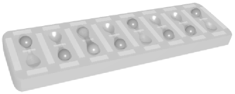
Figure 2: Quantum (double) dots

3 Quantum signal propagation in nanosystems

Let us discuss now application of some ideas to next generations of nanotechnologies. Such devices are still in a state of development and it may be reasonable to pay attention to processes in biosystems. Recent time active research is carried out with respect to descendants of most ancient “nanodevices” existing on the Earth about three milliards years or so.

It is the light-harvesting complex of some microorganisms. The importance of quantum effects for this case is already almost impossible to deny. The significant contribution for understanding here is due to works with participation of experts in quantum theory of information [8, 9, 10, 11].

Let us consider a problem of the effective transfer of absorbed photon energy to different elements of a nanosystem. In the biological systems mentioned above the effectiveness may be about 99%. It is astonishing with taking into consideration of quantum uncertainty, because it apparently should hinder the optimal transfer.

Yet biophysical processes in such systems formally look as not relevant with information transfer, a set of problems and methods applied there are very similar with the statement of a question about an effective transmission of signals in a nanodevice with taking into account of quantum effects. E.g., in paper [9] is suggested a transfer model based on a quantum analogue of the random walk. In the classical case a chaotic motion may be considered as a quite effective way of a transport in complicated compact systems.

Uncertainty of positions and trajectories in quantum mechanics needs for the special consideration. There is well known approach with the suggestion about state localization due to the interaction with the environment. It is one possible explanation of the transition from quantum to classical world [12]. Related ideas about decoherence assisted transport may be more or less directly used in some models about effective energy transfer in the light-harvesting complexes [9, 10].

Some classical models are tested very well for the macroscopic level and it is not clear at that scale they are still work for nanosystems. It is reasonable to check a possibility of description of the effective transfer without appealing to semi-empiric regularities acting on the boundary between quantum and classical world [12].

Indeed, the possibility of the “perfect” transfer of an excitation in “purely” quantum approach was also found recently [13]. Similar methods was only briefly mentioned in the relation with the biophysical systems discussed above [11].

In the works [14, 15] were also considered some aspects of this approach, appropriate to the present discussion. It can be said, the model of perfect transfer is an analogue of shift register: $10000000$ $\rightarrow$ $01000000$ $\rightarrow$ $\ldots$ $\rightarrow$ $00000001$. Here unit corresponds to the excited state. Coefficients describing strength of interactions between adjacent nodes of the chain may be chosen in such a way, to ensure localization of excitation only for two ends of chain and perfect transfer from first to last node [13].

Let us recollect some essential ideas. The quantum information science is most often related with quantum systems with finite number of (basic) states and it was quite clear from examples with qubits above. In more general case the term qudit is often used for a quantum system with $d$ states, e.g., a particle with spin $s$ corresponds to $d=2s+1$. Qubit is the particular case with $d=2$ and $s=1/2$.

Other model of qudit is some particle in a lattice with $d$ locations. Two simple examples with $d$ nodes are ring (Figure 3a) [16, Chap. 15-4] and a line (Figure 3b) [16, Chap. 15-5]. If we consider a single electron in such a circular or linear system, the wave numbers $k_{j}$ of stationary states may be expressed as $k_{j}b=2\pi j/d$ and $k_{j}b=\pi j/(d+1)$ respectively [16, Chap. 15]. The energies in both cases are

$$E_{j}=E_{0}-2A\cos(k_{j}b).$$ (1)

Here $b$ is distance between atoms and $A$ is amplitude of transition.

a)    b)

Figure 3: Models with lattices

4 Understanding perfect state transfer

Such chains may be used for quantum communications [17], but a nonlinear dispersion law like Eq. (1) may be considered as a certain obstacle for the good transmission. Already mentioned earlier perfect scheme of transport has varying amplitudes of transition [13]

$$A_{j}=A\sqrt{j\,(d-j)}.$$ (2)

Such a model may appear more natural, if to consider a simpler equivalent [14]. Indeed, in the continuous case the ideal transmission of a signal might be obtained with the linear law of dispersion $E(k)\propto k$. For the quantum case with the discrete lattice there is similar approach.

Let us denote a state with occupation of only $l$’th node as $|l\rangle$, cf [16, Figure 13-1]. A spin chain also may be used [13] instead of the lattice with $d$ states. Yet, the chain has $2^{d}$ basic states (Figure 1a), only $d$-dimensional subspace is used [13] and it illustrates rather standard correspondence between such lattices [16, Chap. 13] and spin waves in chains with exchange interaction [16, Chap. 15].

If to consider a ring (Figure 3a) with $d$ nodes, the ideal scheme of transfer could be described via cyclic shift operator

$${\bf U}:|l\rangle\mapsto|\,l+1\mod d\rangle,\quad l=0,\ldots,d-1.$$ (3)

Eigenvectors and eigenvalues of the operator may be simply found

$${\bf U}|\kappa_{j}\rangle=\zeta_{j}|\kappa_{j}\rangle,\quad\zeta_{j}=\exp\bigl{(}\frac{2\pi i}{d}\,j\bigr{)},$$ (4)

$$|\kappa_{j}\rangle=\frac{1}{\sqrt{d}}\sum_{l=0}^{d-1}\exp\bigl{(}\frac{2\pi i}{d}\,lj\bigr{)}\,|l\rangle$$ (5)

and produce “momentum” basis with $d$ states.

Similar states were already mentioned above in relation with a “molecular” ring, Figure 3. These states had the fixed wave number $k$. A simplest analogy of a continuous model with linear dispersion may be provided by Hamiltonian with eigenvectors $|\kappa_{j}\rangle$ described by Eq. (5) and equidistant eigenvalues, i.e.,

$${\bf H}\,|\kappa_{j}\rangle=\hbar\theta j\,|\kappa_{j}\rangle$$ (6)

with unessential constant $\theta$.

Evolution of a system due to such Hamiltonian in the same basis may be expressed via a diagonal matrix, i.e.,

$$|\kappa_{j}\rangle\mapsto\exp(-i\theta jt)|\kappa_{j}\rangle.$$ (7)

It is convenient to choose time step

$$\Delta t=\frac{2\pi}{\theta\,d},$$ (8)

because the matrix of evolution of the quantum system for such a time period coincides with introduced earlier Eq. (3) matrix of cyclic shift

$${\bf U}=\exp(\frac{{\bf H}\Delta t}{i\hbar}),$$ (9)

i.e., it is expressed in basis $|\kappa_{j}\rangle$ as

$${\bf U}:|\kappa_{j}\rangle\mapsto\exp\bigl{(}\frac{2\pi i}{d}\,j\bigr{)}\,|\kappa_{j}\rangle.$$ (4^′)

So, on the one hand, ${\bf U}$ is a discrete analogue of operator with linear dispersion, on the other one, it ensures perfect transmission Eq. (3) of local state along chain.

The advantage of such approach is very clear law of evolution Eq. (3), but in the basis $|l\rangle$ there is no simple expression like Eq. (6) for Hamiltonian used in Eq. (9). The Hamiltonian in such basis may be found [14, Eq. (10)], but it has nonzero values of transition amplitudes for any two sites, unlike initial models with nonzero elements only for adjacent locations [16].

It is useful to look for Hamiltonians with the same equidistant spectra, but nonzero values of transition only for $j\pm 1$. Analogues of angular momentum components operators like ${\bf J}_{x}$ or ${\bf J}_{y}$ have necessary properties and in [13] was used such a formal Hamiltonian with only nonzero elements $\grave{H}_{j,j\pm 1}$ corresponding to Eq. (2) and proportional to ${\bf J}_{x}$ for some fictitious particle with spin $s=(d-1)/2$

$$\grave{\bf H}=\vartheta\hbar\!\!\begin{pmatrix}0\ \quad\sqrt{d-1}\ \quad 0&\cdots\!&0\ \ \qquad 0\\ \sqrt{d-1}\quad 0\ \sqrt{2(d-2)}&\cdots\!&0\ \ \qquad 0\\ 0\ \ \sqrt{2(d-2)}\ \ 0&\cdots\!&0\ \ \qquad 0\\ \dotfill\ddots&\ddots&\ddots\dotfill\\ 0\ \ \qquad 0\ \ \qquad 0\,&\cdots\!&\ \ 0\ \ \sqrt{d-1}\\ 0\ \ \qquad 0\ \ \qquad 0\,&\cdots\!&\sqrt{d-1}\ \ 0\ \ \end{pmatrix}.$$ (10)

Evolution of a system with such a Hamiltonian is described by operator

$${\bf R}(t)=\exp(\frac{\grave{\bf H}t}{i\hbar})=\exp(\frac{\vartheta{\bf J}_{x}t}{i\hbar}).$$ (11)

It coincides with a revolution generated in $d$-dimensional representation of rotation group by ${\bf J}_{x}$ and familiar from theory of angular momentum [16, Chapt. 18]. Here is discussed a linear chain, but due to such representation there is an analogy with a ring — it can be considered formally as a chain with reflection on the boundaries.

There is a subtle problem, because instead of one-way transmission the state is rather circulating between two ends of the lattice with period $\pi/\vartheta$. It may be resolved by controlled state transfer, like quantum bots (qubots) discussed in [14] or more cumbersome schemes.

The consideration above illustrates application of general methods for description of information transfer in the different types of quantum wires. From the one hand it takes into account quite specific properties of quantum systems, from the other one it draws a parallel with the traditional information science.

5 Weyl commutation relations

Let us return to the question about problems with quantum uncertainty. The operator of shift ${\bf U}$ Eq. (3) is an important attribute of quantum mechanics and used in so-called Weyl commutation relations [18].

For the continuous case such a formalism has the direct correspondence with the Heisenberg commutation relations [18, 19]. Indeed in some cases it is necessary to use the Heisenberg uncertainty relation with proper care due to subtleties with definition of domains of operators [19, 20], e.g., for a ring with the periodic coordinate $0\leq q<2\pi$ the value $\Delta q$ is always finite, but $\Delta p=0$ for eigenfunctions of ${\bf p}$, i.e.,

$$u_{k}(q)=(2\pi)^{-1/2}\exp(ikq),$$ (12)

and so $\Delta p\,\Delta q=0$ [19, 20]. Here $|u_{k}(q)|^{2}$ is constant and $\Delta q=\pi/\sqrt{3}$ — it coincides with the standard deviation of the random variable $0\leq q<2\pi$ with the uniform distribution.

More details may be found in [20, Chapt. 4-3] (with notation $\theta$ and $p_{\theta}$ for ${\bf q}$ and ${\bf p}$ respectively). It should be mentioned, that operators ${\bf q}$ and ${\bf p}$ above were not “usual” coordinate and momentum for a particle on a line with uncertainty relation $\Delta p\,\Delta q\geq\hbar/2$. For a line $\Delta q$ is not limited by some fixed value and for $\Delta p\to 0$ we would have “unrestricted” plane waves instead of Eq. (12), i.e., $\Delta q\to\infty$. Here the limit is an uniform distribution on an infinite line $-\infty<q<\infty$, instead of a bounded ring.

Qubit and qudit are said to be “discrete quantum variables” widely used in the quantum information science. For such systems the problem with proper definition of coordinate, momentum operators and analogues of uncertainty relations could look even worst, than for continuous ring, but Weyl quantization [18] may help to resolve that. The idea is to consider exponents of coordinate and momentum operators [18, 19]

$${\bf U}(a)=\exp(ia{\bf p}),\quad{\bf V}(b)=\exp(ib{\bf q}).$$ (13)

In the continuous case the actions of such operators on a wave function $\psi(x)$ are represented as

$${\bf U}(a)\psi(x)=\psi(x+\hbar a),\quad{\bf V}(b)\psi(x)=e^{ibx}\psi(x),$$ (14)

and direct consequence of Heisenberg commutation relation

$$[{\bf q},{\bf p}]\equiv{\bf q}{\bf p}-{\bf p}{\bf q}=i\hbar$$ (15)

is Weyl commutation relation [18, 19]

$${\bf U}(a){\bf V}(b)=\exp(i\hbar ab){\bf V}(b){\bf U}(a).$$ (16)

Such a scheme has some advantage because Weyl pair ${\bf U}$, ${\bf V}$ with appropriate properties may be formally written even if ${\bf p}$ and ${\bf q}$ are not (well) defined. It may be even used for discrete quantum variables [18] and it was already reproduced above in example with operator of shift U Eq. (3). The second operator in this case is

$${\bf V}:|l\rangle\mapsto\exp\bigl{(}\frac{2\pi i}{d}\,l\bigr{)}\,|l\rangle.$$ (17)

So, ${\bf U}$ and ${\bf V}$ are $d{\times}d$ matrixes with commutation relation

$${\bf U}{\bf V}=\exp\bigl{(}\frac{2\pi i}{d}\bigr{)}\,{\bf V}{\bf U}.$$ (18)

These matrixes together with relation Eq. (18) were introduced by Weyl [18]. Really, the “shift” ${\bf U}$ and “clock” ${\bf V}$ matrixes were considered even earlier in few works of J. J. Sylvester around 1882–1884. In quantum information science they are also known as “generalized Pauli matrixes” with an alternative notation ${\bf X}$ and ${\bf Z}$ [21].

Other examples may be found elsewhere [22]. Let us only consider less formally questions about uncertainty for discrete quantum variables. Famous Stern-Gerlach experiment demonstrates only two possible projections on some axis for spin one-half. For spin $s$ there are $2s+1$ projections. It is just obvious statement about quantization of angular momentum.

A belief about inevitable problems with quantum transport due to uncertainties of trajectories related with lack of examples with similar effects for some spatial properties of quantum systems. It is more common to expect quantization for energy levels, angular momentum, etc. Yet, in quantum information science were quite natural formal models with discrete spatial variables, e.g., quantum cellular automata, quantum lattice gases [23, 24], etc.

6 Conclusion

The quantum information technologies may be useful for construction of difficult nano-technology devices, because they are providing universal and compact way of understanding different processes with “systems of quantum systems.” It is an analogy with the application of usual information technologies for description in symbolic form of classical processes and objects.

In the paper were recollected few simple models: the representation of data by qubits and signal transfer in small quantum systems. These models may be quite familiar in area of quantum computing, but it should be emphasized, that main purpose of present work — is not theory of quantum algorithms adapted for cryptography. Even usual electronic computers were initially constructed for code-breaking and plain calculations, but nowadays they work as well in absolutely different areas.

It should be mentioned also, that this presentation is not concentrated on restricted question, how nanotechnologies could help to build a quantum computer to crack some ciphers. It is rather analyzed, how “quantum-computer-type of thinking” may help to understand and control nano-scale systems and devices.

References

- [1] R. P. Feynman, “There’s plenty of room at the bottom”, Engineering & Science 23(5), p. 22, 1960.
- [2] R. P. Feynman, “Simulating physics with computers,” Int. J. Theor. Phys. 21, p. 467, 1982.
- [3] N. Gisin, “Non-realism : deep thought or a soft option ?”, arXiv:0901.4255 [quant-ph], 2009.
- [4] A. Yu. Vlasov, “Quantum mechanics and nonlocality: In search of instructive description,” arXiv:0901.4645 [quant-ph], 2009.
- [5] C. H. Bennett, “Logical reversibility of computation,” IBM J. Res. Dev. 17, p. 525, 1973.
- [6] P. A. Benioff, “Quantum mechanical Hamiltonian models of discrete processes that erase their own histories: Application to Turing machines,” Int. J. Theor. Phys. 21, p. 177, 1982.
- [7] R. Hughes, G. Doolen, D. Awschalom, C. Caves, M. Chapman, R. Clark, D. Cory, D. DiVincenzo, A. Ekert, P. C. Hammel, P. Kwiat, S. Lloyd, G. Milburn, T. Orlando, D. Steel, U. Vazirani, K. B. Whaley, and D. Wineland, A quantum information science and technology roadmap, v 2.0, ARDA, Washington, D.C., 2004.
- [8] A. Olaya-Castro, C. F. Lee, F. F. Olsen, and N. F. Johnson, “Efficiency of energy transfer in a light-harvesting system under quantum coherence,” Phys. Rev. B 78:085115, 2008.
- [9] M. Mohseni, P. Rebentrost, S. Lloyd, and A. Aspuru-Guzik, “Environment-assisted quantum walks in photosynthetic energy transfer,” J. Chem. Phys. 129:174106, 2008.
- [10] F. Caruso, A. W. Chin, A. Datta, S. F. Huelga, and M. B. Plenio, “Highly efficient energy excitation transfer in light-harvesting complexes,” J. Chem. Phys. 131:105106, 2009.
- [11] M. Sarovar, A. Ishizaki, G. R. Fleming, and K. B. Whaley, “Quantum entanglement in photosynthetic light harvesting complexes,” arXiv:0905.3787 [quant-ph], 2009.
- [12] W. H. Zurek, “Decoherence, einselection, and the quantum origins of the classical,” Rev. Mod. Phys. 75, p. 715, 2003.
- [13] M. Christandl, N. Datta, A. Ekert, and A. J. Landahl, “Perfect state transfer in quantum spin networks,” Phys. Rev. Lett. 92:187902, 2004.
- [14] A. Yu. Vlasov, “Programmable quantum state transfer,” arXiv:0708.0145 [quant-ph], 2007.
- [15] A. Yu. Vlasov, “Quantum mechanics and some properties of nano-scale cybernetics devices,” International Forum Rusnanotech’08, Moscow, 2008. A. Yu. Vlasov, “Quantum information science and nanotechnology,” arXiv:0903.1204 [quant-ph], 2009.
- [16] R. P. Feynman, R. B. Leighton, and M. Sands, The Feynman lectures on physics. Vol. 3. Quantum mechanics, Addison-Wesley, Reading, MA, 1965.
- [17] S. Bose, “Quantum communication through an unmodulated spin chain,” Phys. Rev. Lett. 91:207901, 2003.
- [18] H. Weyl, The theory of groups and quantum mechanics, Dover Publications, New York, 1931.
- [19] N. N. Bogoliubov, A. A. Logunov, A. I. Oksak, I. T. Todorov, General principles of quantum field theory, Nauka, Moscow, 1987; Kluwer Academic Publishers, Dordrecht, 1990.
- [20] A. Peres, Quantum theory: Concepts and methods, Kluwer Academic Publishers, Dordrecht, 1993.
- [21] D. Gottesman, “Fault-tolerant quantum computation with higher-dimensional systems,” Lect. Not. Comp. Sci. 1509, p. 302, 1999.
- [22] A. Yu. Vlasov, “Quantum information processing with low-dimensional systems,” in Quantum information processing: From theory to experiment, edby D. G. Angelakis, M. Christandl, A. Ekert, A. Kay, and S. Kulik, p. 103, IOS Press, Amsterdam, 2006.
- [23] S. Richter and R. F. Werner, “Ergodicity of quantum cellular automata,” J. Stat. Phys. 82, 963, 1996.
- [24] D. A. Meyer, “From quantum cellular automata to quantum lattice gases,” J. Stat. Phys. 85, 551, 1996.