Anderson localization of classical waves in weakly scattering metamaterials
Abstract
We study the propagation and localization of classical waves in one-dimensional disordered structures composed of alternating layers of left- and right-handed materials (mixed stacks) and compare them with structures composed of different layers of the same material (homogeneous stacks). For weakly scattering layers, we have developed an effective analytical approach and have calculated the transmission length within a wide range of the input parameters. This enables us to describe, in a unified way, the localized and ballistic regimes as well as the crossover between them. When both refractive index and layer thickness of a mixed stack are random, the transmission length in the long-wave range of the localized regime exhibits a quadratic power wavelength dependence with different coefficients of proportionality for mixed and homogeneous stacks. Moreover, the transmission length of a mixed stack differs from the reciprocal of the Lyapunov exponent of the corresponding infinite stack. In both the ballistic regime of a mixed stack and in the near long-wave region of a homogeneous stack, the transmission length of a realization is a strongly fluctuating quantity. In the far long-wave part of the ballistic region, the homogeneous stack becomes effectively uniform and the transmission length fluctuations are weaker. The crossover region from the localization to the ballistic regime is relatively narrow for both mixed and homogeneous stacks. In mixed stacks with only refractive-index disorder, Anderson localization at long wavelengths is substantially suppressed, with the localization length growing with wavelength much faster than for homogeneous stacks. The crossover region becomes essentially wider and transmission resonances appear only in much longer stacks. The effects of absorption on one-dimensional transport and localization have also been studied, both analytically and numerically. Specifically, it is shown that the crossover region is particularly sensitive to losses, so that even small absorption noticeably suppresses frequency dependent oscillations in the transmission length. All theoretical predictions are in an excellent agreement with the results of numerical simulations.
pacs:
42.25.Dd,42.25.FxI Introduction
Metamaterials are artificial structures having negative refractive indices for some wavelengths Veselago . While natural materials having such properties are not known, it was the initial paper Pendry that sought to realize artificial metamaterials which triggered the rapidly increasing interest in this topic. Over the past decade, the physical properties of these structures, and their possible applications in modern optics and microelectronics, have received considerable attention (see e.g. Refs Sok ; Bliokh ; classification ; Shalaev ). The reasons for such interest are their unique physical properties, their ability to overcome the diffraction limit Veselago ; Pendry , and their potential role in cloaking Schurig , the suppression of spontaneous emission rate emis , and the enhancement of quantum interference inter , etc.
Until recently, most studies considered only ideal systems and did not address the possible effects of disorder. However, real metamaterials are always disordered, at least, in part, due to fabrication errors. Accordingly, the study of disordered metamaterials is not just an academic question but is also relevant to their application. The first step in this direction was made in Ref. defect where it was shown that the presence of a single defect led to the appearance of a localized mode. A metamaterial with many point-like defects was considered in Ref. Gorkunov where it was demonstrated that even weak microscopic disorder might lead to a substantial suppression of wave propagation through a metamaterial over a wide frequency range.
The next steps in this direction focused on the study of localization in metamaterials. Anderson localization is one of the most fundamental and fascinating phenomenon of the physics of disorder. Predicted in the seminal paper And for spin excitations, it was extended to the case of electrons and other one-particle excitations in solids, as well as to electromagnetic waves (see, e.g., Refs. john84 ; LGP ; Ping91 ; FG ; GMP ; Sheng06 ), becoming a paradigm of modern physics.
Anderson localization results from the interference of multiply scattered waves, manifesting itself in a most pronounced way in one-dimensional systems LGP ; FG , in which all states become localized Mott so that the envelope of each state decays exponentially away from a randomly located localization center LGP . The rate of this decay is non-random and is called the Lyapunov exponent, , the reciprocal of which determines the size of the area of localization.
In a finite, but sufficiently long, disordered sample, the localization manifests itself in the fact that the frequency dependent transmission amplitude is (typically) an exponentially decreasing function of the sample size. The average of this decrement is a size-dependent quantity, whose inverse (i.e., reciprocal) is termed the transmission length, . In the limit as the sample becomes of infinite length, the decrement tends to a constant non-random value. The reciprocal of this value determines another characteristic spatial scale of the localized regime, which is the localization length, . It is commonly accepted in both the solid state physics and optical communities, that the inverse of the Lyapunov exponent, and the localization length, are always equal. While this is true for media with a continuous spatial distribution of the random dielectric constant, in the case of randomly layered samples, the situation, as we show in this paper, is more complicated. In particular, the inverse of the Lyapunov exponent by itself, calculated, for example, in Ref. Israilev , does not provide comprehensive information about the transport properties of disordered media. Furthermore, it is unlikely that it can be measured directly, at least in the optical regime.
The first study of localization in metamaterials was presented in Ref. Lyapunov where wave transmission through an alternating sequence of air layers and metamaterial layers of random thicknesses was studied. Localized modes within the gap were observed and delocalized modes were revealed despite the one-dimensional nature of the model. A more general model of alternating sequences of right- and left-handed layers with random parameters was studied in Ref. we . There, it has been shown that in mixed stacks (M-stacks) with fluctuating refractive indices, localization of low-frequency radiation was dramatically suppressed so that the localization length exceeded that for homogeneous stacks (H-stacks), composed solely of right- or left-handed slabs, by many orders of magnitude and scaling as or even higher powers of wavelength (in what follows we refer to this result as the anomaly), in contrast to the well-known dependence observed in H-stacks Baluni . As noted in Ref. we , a possible physical explanation of this is the suppression of phase accumulation in M-stacks, related to the opposite signs of the phase and group velocities in left- and right-handed layers. Scaling laws of the transmission through a similar mixed multilayered structure were studied in Ref. random . There, it was shown that the spectrally averaged transmission in a frequency range around the fully transparent resonant mode decayed with the number of layers much more rapidly than in a homogeneous random slab. Localization in a disordered multilayered structure comprising alternating random layers of two different left-handed materials was considered in Ref. single , where it was shown that within the propagation gap, the localization length was shorter than the decay length in the underlying periodic structure, and the opposite of that observed in the corresponding random structure of right-handed layers.
In this paper, we study the wave transmission through disordered M- and H-stacks of a finite size composed of a weakly scattering right- and left-handed layers. In the framework of the weak scattering approximation (WSA), we have developed a unified theoretical description of the transmission and localization lengths over a wide wavelength range, allowing us to explain the pronounced difference in the transmission properties of M- and H-stacks at long wavelengths.
When both refractive index and layer thickness of the mixed stack are random, the transmission length in the long wavelength part of the localized regime exhibits a quadratic power law dependence on wavelength with different constants of proportionality for mixed and homogeneous stacks. Moreover, in the localized regime, the transmission length of a mixed stack differs from the reciprocal of the Lyapunov exponent of the corresponding infinite stack (to the best of our knowledge, in all one-dimensional disordered systems studied till now these two quantities always coincide).
Both M- and H-stacks demonstrate a rather narrow crossover from the localized to the ballistic regime. The H-stack in the near ballistic region, and the M-stack in the ballistic region are weakly scattering disordered stacks, while in the far ballistic region, the H-stack transmits radiation as an effectively uniform medium.
We also consider the effects of loss and show that absorption dominates the effects of disorder at very short and very long wavelengths. The crossover region is particularly sensitive to losses, so that even small absorption suppresses oscillations in the transmission length as a function of frequency.
All of the theoretical results mentioned above are confirmed by, and are shown to be in excellent agreement with, the results of extensive numerical simulation.
In M-stacks with only refractive index disorder, Anderson localization and transmission resonances are effectively suppressed and the crossover region between the localized and ballistic regimes is orders of magnitude greater. A more detailed study of the -anomaly shows that the genuine wavelength dependence of the transmission length is not described by any power law and rather is non-analytic in nature.
II Model
II.1 Mixed and homogeneous stacks
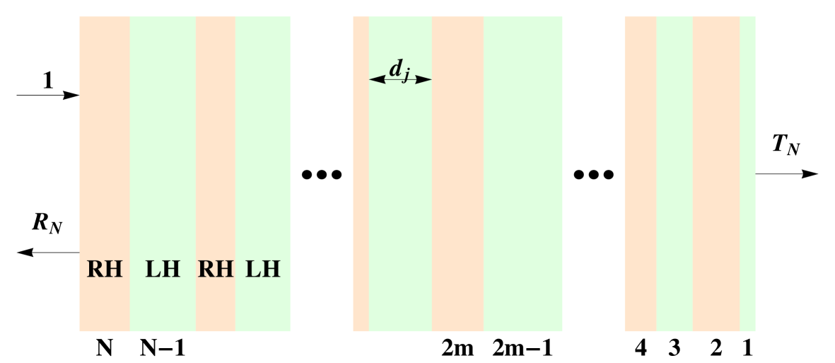
We consider a one-dimensional alternating M-stack, as shown in Fig. 1. It comprises disordered mixed left- () and right- () handed layers, which alternate over its length of layers, where is an even number. The thicknesses of each layer are independent random values with the same mean value . In what follows, all quantities with the dimension of length are measured in units of . In these units, for the thicknesses of a layer we can write
where the fluctuations of the thickness, are zero-mean independent random numbers.
We take the magnetic permeability for right-handed media to be and for metamaterials to be , while the dielectric permittivity is
where the upper and lower signs respectively correspond to normal (right-handed) and metamaterial (left-handed) layers. The refractive index of each layer is then
where all and absorption coefficients of the slabs, , are independent random variables. With this, the impedance of each layer relative to the background (free space) is
with the same choice of the sign.
We begin with the general case when both types of disorder (in refractive index and in thickness) are present. Two particular cases, each with only one type of disorder, are rather different. In the absence of absorption, the M-stack with only thickness disorder is completely transparent, a consequence of . However, the case of only refractive-index disorder is intriguing because, as is shown below, such mixed stacks manifest a dramatic suppression of Anderson localization in the long wave region we .
Although localization in disordered H-stacks with right-handed layers has been studied by many authors Baluni ; deSterke ; Asatrian2 ; Sheng06 ; Luna , here we consider this problem in its most general form and show that the transmission properties of disordered H-stacks are qualitatively the same for stacks comprised of either solely left- or right-handed layers.
II.2 Transmission: localized and ballistic regimes
We introduce the transmission length of a finite random configuration as
| (1) |
where is the random transmission coefficient of a sample of the length As a consequence of the self-averaging of ,
| (2) |
This means that for a sufficiently long stack (in the localized regime) the transmission coefficient is exponentially small .
In what follows, we consider stacks composed of layers with low dielectric contrasts, i.e, so that the Fresnel reflection coefficients of each interface, and of each layer, are much smaller than Here, a thin stack comprising a small number of layers is almost transparent. In this, the ballistic regime, the transmission length takes the form
| (3) |
involving the average reflection coefficient Rytov , which is valid in the case of lossless structures. This follows directly from Eq. (1) by virtue of the conservation relationship, . Thus, in the ballistic regime,
| (4) |
where the length in this equation is termed the ballistic length.
Accordingly, in studies of the transport of the classical waves in one-dimensional random systems, the following spatial scales arise in a natural way:
Note that in the case of absorbing stacks (), the right hand side of Eq. (1) defines the attenuation length, , which incorporates the effects of both disorder and absorption.
In what follows, we show that contrary to commonly accepted belief, the quantities , , and are not necessarily equal, and, under certain situations, can differ noticeably from each other.
In this paper, we study mainly the transmission length defined above by Eq. 1. This quantity is very sensitive to the size of the system and therefore is best suited to the description of the transmission properties in both the localized and ballistic regimes. More precisely, the transmission length coincides either with the localization length or with the ballistic length, respectively in the cases of comparatively thick (localized regime) or comparatively thin (ballistic regime) stacks. That is,
Another argument supporting our choice of the transmission length as the subject of investigation is that it can be found directly by standard transmission experiments, while measurements of the Lyapunov exponent call for a much more sophisticated arrangement.
III Analytical studies
III.1 Weak scattering approximation
The theoretical analysis involves the calculation of the transmission coefficient using a recursive procedure. Consider a stack which is a sequence of layers enumerated by index from at the rear of the stack through to at the front. The total transmission ( and reflection () amplitude coefficients of the stack satisfy the recurrence relations
| (5) | |||||
| (6) |
for , in which both the input and output media are free space. In Eqs (5) and (6), the amplitude transmission () and the reflection () coefficients of a single layer are given by
| (7) | |||||
| (8) |
Here, , and denotes the dimensionless free space wavelength. While the sign of the phase shift across each slab varies according to the handedness of the material, the Fresnel interface coefficient given by
| (9) |
depends only on the relative impedance of the layer , a quantity whose real part is positive, irrespective of the handedness of the material.
Equations (5)-(9) are general and provide an exact description of the system and will be used later for direct numerical simulations of its transmission properties.
It was mentioned previously that we consider the special case of weak scattering for which the reflection from a single layer is small. i.e., . This occurs either for weak disorder, or for strong disorder provided that the wavelength is sufficiently long. The transmission length then follows from
| (11) | |||||
| (12) |
In deriving Eq. (12), we omit the first-order term since it contributes only to the second order of already after the first iteration. Then, by summing up logarithmic terms (11), we obtain
| (13) |
This equation enables us to derive a general expression for the transmission length which is valid in all regimes (see the next Section). However, the ballistic length , according to Eq. (4) (and the average reflection coefficient as well), is determined only by the total reflection amplitude in the case of lossless strutures. In the ballistic regime, this amplitude coefficient, to the necessary accuracy, is given by
| (14) |
III.2 Mixed stack
III.2.1 General Approach
From here on, we assume that the random variables of left-handed or right-handed layers, , and are identically distributed according to the corresponding probability density functions. This enables us to express all of the required quantities via the transmission and reflection amplitudes of a single right-handed or left-handed layer, , , and also to calculate easily all of the necessary ensemble averages.
The average of the first term in Eq. (13) can be written as
Next, we split the second term of Eq. (13) into two parts
where
comprising contributions to the depletion of the transmitted field due to two pass reflections respectively between slabs of different materials (i.e., of opposite handedness), and between slabs of the same material (i.e., of like handedness). Averaging these expressions, we obtain
| (15) | |||||
| (16) |
where
| (17) |
The resulting transmission length is determined by the equation
| (18) |
In the lossless case (), the first term on the right hand side of Eq. (18) corresponds to the so-called single-scattering approximation, which implies that multi-pass reflections are neglected so that the total transmission coefficient is approximated by the product of the single layer transmission coefficients, i.e.,
In the case of very long stacks (i.e., as the length ), we can replace the arithmetic mean, , by its ensemble average On the other hand, in this limit the reciprocal of the transmission length coincides with the localization length. Using the energy conservation law, , which applies in the absence of absorption, the inverse single-scattering localization length may be written as
| (19) |
and is proportional to the mean reflection coefficient of a single random layer LGP ; Liansky-1995 . The corresponding modification of Eq. (18) then reads
| (20) |
Here, the first term corresponds to the single-scattering approximation, while the next two terms take into account the interference of multiply scattered waves as well as the dependence of the transmission length on the stack size. Note that Eq. (20) is appropriate only for lossless structures. In the presence of absorption, Eq. (18) should be used instead.
III.2.2 Transmission length
From this point on, we assume that the statistical properties of the right-handed and left-handed layers are identical. As a consequence of this symmetry, the following relations hold for any real-valued function in either the lossless or absorbing cases:
| (21) |
Therefore, and are the complex conjugates of and , and is real quantity, as are both averages and .
Accordingly, as a consequence of the left-right symmetry (21), the transmission length of a M-stack depends only on the properties of a single right-handed layer and may be expressed in terms of three averaged characteristics: , , and (in which we omit the subscript ).
With these observations, the transmission length of a finite length M-stack may be cast in the form:
| (22) |
where
| (23) |
and
| (24) | |||||
are, as we will see below, the inverse localization and inverse ballistic lengths. The function is defined as
| (25) |
and introduces a new characteristic length termed the crossover length
| (26) |
which arises in the calculations in a natural way and, as will be demonstrated below, plays an important role in the theory of the transport and localization in one-dimensional random systems. Equations (22)-(24) completely describe the transmission length of a mixed stack in the weak scattering approximation.
Obviously, the characteristic lengths , , and appearing in Eq. (22) are functions of wavelength. Using straightforward calculations, it may be shown that the first two always satisfy the inequality , while, as we will see, the crossover length is the shortest of the three, i.e., in the long wavelength region.
In the case of a fixed wavelength and a stack so short that , the expansion of the exponent in Eq. (25) yields , in which case the transmission length approaches . Correspondingly, for a sufficiently long stack, , and the transmission length assumes the value of .
In summary,
with the transition between the two ranges of being determined by the crossover length.
While in the lossless case, the ballistic regime occurs when the stack is much shorter than the crossover length (), it is important to note that, in the localization regime, the opposite inequality is not sufficient and the necessary condition for localization is . In what follows, we consider samples of an intermediate length, i.e., .
For a M-stack of fixed size the parameter governing the transmission is the wavelength, and the conditions for the localized and ballistic regimes should be formulated in the wavelength domain. To do this, we introduce two characteristic wavelengths, and defined by the relations
| (27) |
It can be shown that the long wavelength region, , corresponds to localization where the transmission length coincides with the localization length, while in the extremely long wavelength region, , the propagation is ballistic, with the transmission length given by the ballistic length . That is,
| (28) |
When , there exists an intermediate range of wavelengths, , which will be discussed below.
To better understand the physical meaning of the expressions (23) and (24) for the localization and ballistic lengths, we will consider ensembles of random configurations in which the fluctuations and are distributed uniformly over the intervals and respectively, with . The average quantities that arise in Eqs. (23) and (24) are presented in the Appendix. These formulae allow for calculations with an accuracy of order for arbitrary . For the sake of simplicity, we assume that the fluctuations of the refractive index and thickness are of the same order, i.e., so that the dimensionless parameter
is of order of unity. We also neglect the contribution of terms of order higher than .
The short wavelength asymptotic of the localization length is then
| (29) |
In the long wavelength limit, we obtain the following asymptotic forms for the corresponding single layer averages:
| (30) | |||||
| (31) | |||||
| (32) | |||||
Substitution of these expansions into Eq. (24) yields the long wavelength asymptotic of the ballistic length
| (33) |
This asymptotic can be calculated directly from Eq. (4) with the average reflection coefficient, determined from Eq. (14), being
| (34) |
The same substitutions into this equation (34) give the average total reflection coefficient
| (35) |
In the ballistic regime, the final term is negligibly small. This, together with Eq. (4), again results in the value of the ballistic length given in Eq. (33).
Substituting the long wavelength expansions (30)–(32) into Eqs. (23) and (26), we derive the following asymptotic forms for the localization length
| (36) |
and the crossover length
| (37) |
In seeking to compare the result (36) for the localization length with the corresponding long wave asymptotic of the reciprocal Lyapunov exponent, it is important to note that these two quantities are defined in different ways. The localization length is defined by Eq. (2) via the transmittivity on a realization, while the Lyapunov exponent describes an exponential growth of the envelope of a currentless solution far from a given point in which the solution has a given value LGP . We have calculated the long wave asymptotic of the M-stack Lyapunov exponent using the well known transfer matrix approach, assuming the same statistical properties of the modulus of dielectric constant and the thickness of both left- and right-handed layers,
| (38) | |||||
In the case of rectangular distributions of the fluctuations of the dielectric constants and thicknesses, this result reduces to
| (39) |
(we neglected the small corrections proportional to ). Thus, the disordered M-stack in the long wavelength region presents a unique example of a one-dimensional disordered system in which the localization length differs from the reciprocal of the Lyapunov exponent.
The long wavelength asymptotic of the Lyapunov exponent and the asymptotic of the localization length, , Eq. (36) have rather clear physical meaning. Indeed, in the limit , the propagating wave is insensitive to disorder since the disorder is effectively averaged over distances of the order of the wavelength. This means that Anderson localization is absent and the Lyapunov exponent vanishes. For large but finite wavelengths (i.e., small wavenumbers , the Lyapunov exponent is small and, assuming that its dependence on the wavenumber is analytic, we can expand it in powers of . This expansion commences with a term of order since the Lyapunov exponent is real and the wavenumber enters the field equations in the form . Accordingly, in the long wavelength limit, and so .
The behavior of the Lyapunov exponent given by (38) does not depend on the handness of the layers; compare this equation with the corresponding long wave asymptotic obtained in Refs. Ping91 ; single for homogeneous stacks composed of only positive or only negative layers. However, it crucially depends on the propagating character of the field within a given wavelength region. When this region is within the gap of the propagation spectrum of the effective ordered medium, the frequency dependence of the Lyapunov exponent differs from . It takes place, for example, for a stack composed of single negative layers, where only one of two characteristics (, ) is negative single .
The main contribution to the ballistic length (33) is due to the final term in the right hand side of Eq. (24), which corresponds to the single-scattering approximation discussed at the end of the Sec. III.2.1. While the ballistic length follows from the single scattering approximation, the calculation of the localization length (36) is more complex and requires that interference due to the multiple scattering of waves must be taken into account.
In the case under consideration ( and ), the two characteristic wavelengths and (27) for an M-stack of a fixed length size take the form
| (40) | |||||
| (41) |
and are of the same order of magnitude. This means that the transmission length coincides with the localization length (36) for ), and with the ballistic length (33) in the case when .
The crossover between the localized and ballistic regimes occurs for , with the two bounds being proportional to and thus growing as . For long stacks, the transmission length in the crossover region can be described with high accuracy by the general equations (22) and (25), where the ballistic length , the localization length , and the crossover length are replaced by their asymptotic forms (33)–(37). In the case of solely refractive index disorder ( when all thicknesses are set to unity, the ballistic length and the short wavelength asymptotic of the localization length coincide with the limiting values of their counterparts for an M-stack with both refractive index and thickness disorder (33) and (29). However, the corresponding limiting values of the long wavelength localization length and crossover lengths have nothing to do with the genuine behaviour of the transmission length (see Sec. IV.2.1). This means that the weak scattering approximation fails to describe the long wavelength asymptotics of the transmission length in both the localization and crossover regions. This is discussed in greater detail below.
Eqs. (15)–(18) (or Eqs. (22)–(26)) in the symmetric case) completely determine the behaviour of the transmission length for a mixed stack composed of weakly scattering layers. Although has been introduced as a crossover length, the entire region does not necessarily support localization. Correspondingly, the ballistic regime may exist outside the region
All of the results obtained under the symmetry assumption (21) are qualitatively valid in the general case. Indeed, the existence of the crossover (28) is related to the exponential dependence in Eq. (25) with a real and positive crossover length . When the assumption of symmetry no longer holds, this length takes a complex value. However, the quantity in Eq. (16) satisfies (by its definition in Eq. (17)) the evident inequality . Therefore, the corresponding analogue of the function (25) preserves all necessary limiting properties (see the next Sec. III.2.3).
III.2.3 Homogeneous stacks
In this Section, we consider a H-stack composed entirely of normal material layers noting that the behaviour of a H-stack of metamaterial (left-handed) layers alone is exactly the same, a result which may be obtained directly from Eq. (18) by replacing each by , after which any reference to the index may be omitted. The transmission length of an H-stack is then
| (42) |
where the inverse localization length is
| (43) |
Now we consider a H-stack composed of weakly scattering layers. To simplify the discussion, we consider only refractive index disorder (i.e., ). In this case, the asymptotic behavior of the localization length in the short and long wavelength limits are
| (44) |
The main contribution to the localization length is related to the first term in Eq. (43). Thus, the localization length of the H-stack in the long wavelength region is described completely by the single scattering approximation and coincides with the ballistic length (33) of the M-stack.
Using the transfer matrix approach, we can also calculate the long wavelength asymptotic of the Lyapunov exponent for a H-stack . It is described by the same equation (38) as the asymptotic for the M-stack, thus coinciding with the asymptotic of the reciprocal Lyapunov exponent. In recent work Israilev , this coincidence was established analytically in a wider spectral region. However, the numerical calculations intended to confirm this result are rather unconvincing. Indeed, the numerically obtained plots demonstrate strong fluctuations (of the same order as the mean value) of the calculated quantity, while the genuine Lyapunov exponent is non-random and should be smooth without any additional ensemble averaging mentioned by the authors.
If we cast in the second term of Eq. (42) in the form we see that the crossover length of the H-stack is
with its long wavelength asymptotic, according to Eq. (32), being
| (45) |
Here, the crossover length is proportional to the wavelength, in stark contradistinction to the situation for M-stacks, in which the crossover length is proportional to .
To consider this further, we define the characteristic wavelengths and by the expressions (27). For a H-stack, these lengths are
| (46) |
Evidently, the second characteristic wavelength is always much larger than the first . As a consequence, the long wavelength region, where the ballistic regime is realized, can be divided into two subregions. The near subregion (moderately long wavelengths) is bounded by the characteristic wavelengths
The main contribution to the ballistic length in the near ballistic region, is due to the first term in Eq. (43). Thus the ballistic length has the same wavelength dependence as the localization length (44)
and is well described by the single scattering approximation (19). For a H-stack , the transition from the localized to the ballistic regime at is not accompanied by any change of the wavelength dependence of the transmission length. This change can occur at much longer wavelengths in the far long wavelength subregion.
To derive the ballistic length in the far long wavelength region, we may proceed in a similar manner to that outlined in the case of a M-stack and expand the exponent in Eq. (42). However, because in this expression is complex, the situation is more complicated than was the case for the M-stack. In particular, the first two terms of the expansion do not contribute to the ballistic length. Taking account of the second order leads to the following expression for the ballistic length, in the far long wavelength region
| (47) |
In the case of a relatively short H-stack the contribution of the first term in the right hand side of this equation dominates, and hence the transition from the near to the far subregions is not accompanied by any change in the analytical dependence on the wavelength. The ballistic length is thus described by the same wavelength dependence over the entire ballistic region
| (48) |
For sufficiently long H-stacks in the far long wavelength region, the second term is dominant and so
| (49) |
Thus, the wavelength dependence of the ballistic length of a sufficiently long H-stack is
| (50) |
The same result for the ballistic length also follows from Eq. (4) with Eq. (14), in the case of a homogeneous stack, yielding
| (51) |
In the long wave limit this leads to
| (52) |
The final term in Eq. (51) differs from the final term in Eq. (34) and, therefore, in contrast to the M-stack, its contribution to the total reflection coefficient can be of the order of, or larger than, that of the first term. This together with Eq. (4) is equivalent to the result in Eqs. (48) and (50), and is applicable to short and long stacks respectively.
The far long wavelength ballistic asymptotic (49) has a simple physical interpretation. Indeed, in this subregion, the wavelength essentially exceeds the stack size and so we may consider the stack as a single weakly scattering uniform layer with an effective dielectric permittivity In this case, the ballistic length of the stack according to Eq.(4) is
| (53) |
where
| (54) |
is the long wavelength form of the reflection amplitude for a uniform right-handed stack of the length and constant dielectric permittivity (with ). In the case of a uniform left-handed stack, the value of the reflection coefficient should be
| (55) |
in which the value of is now negative (with ).
To calculate the effective parameters, we use Eq.(14). Neglecting small fluctuations of the layer thickness, the single layer reflection amplitude in the long wavelength limit reads
| (56) |
The total reflection amplitude for a stack of length is
| (57) |
corresponding to the effective dielectric permittivity determined by the expression
| (58) |
For sufficiently long stacks, the right hand side of this equation can be replaced by the ensemble average and hence
| (59) |
This expression is similar to that of the two-dimensional case for disordered photonic crystals reported in Ref. Asatryan99 . The same considerations as above, but for a homogeneous stack composed entirely with disordered metamaterial slabs, also lead to an effective value of the permittivity,
| (60) |
Eq. (58), together with Eqs (53), (54), leads immediately to the far long wavelength ballistic length (49). We emphasize that because of the effective uniformity of the H-stack in the far ballistic region, the transmission length on a single realization is a less fluctuating quantity. In contrast, transmission length for H-stacks fluctuates strongly in the near ballistic region, as indeed it does over the entire ballistic region for M-stacks.
To characterize the entire crossover region between the two ballistic regimes (50) in greater detail, we return to the general formula (42), in which we represent as . Then, in accordance with Eq. (32), we can write
| (61) |
As a consequence, instead of the result in Eq. (47), we obtain
| (62) |
We note that, strictly speaking, the expansion (61) is valid inside the interval
The second term in Eq. (52) represents standard oscillations of the reflection coefficient of a uniform slab of finite size. In the far long wavelength limit this equation coincides with (47). Thus, Eq. (52) describes the ballistic length over practically the whole ballistic region Moreover, taking into account that the long wavelength asymptotic of the localization length coincides with that of the near long wavelength ballistic length, we see that the right hand side of Eq. (52) serves as an excellent interpolation formula for the reciprocal of the transmission length of a sufficiently long stack () over the entire long wavelength region
III.3 Comparison of the transmission length behaviour in M- and H- stacks
Away from the transition regions, the transmission length can exhibit three types of long wavelength asymptotics described by the right hand sides of Eqs. (33), (36), and (49). The first (33) corresponds to the single scattering approximation where the inverse transmission length is proportional to the average reflection coefficient of a single random layer. In the absence of absorption, this characterizes both the localization and ballistic lengths. The second asymptotic form (36) takes into account the interference of multiply scattered waves and describes the localization length. The third asymptotic (49) corresponds to transmission through a uniform slab with an effective dielectric constant given by Eq. (59) and is relevant only in the ballistic regime.
In the case of a M-stack, the first two expressions (33) and (36) characterize the ballistic and localized regimes respectively, while the third asymptotic is never realized in M-stacks. In relatively short H-stacks (48), the long wavelength behaviour of the transmission length is described by the same dependence (33) in both the localized and ballistic regimes. Finally, in the case of long H-stacks (49), the transmission length follows from Eq. (33) in the localized and near ballistic regimes, while in the far ballistic region it is described by the right hand side of Eq. (49).
These results predict the existence of a different wavelength dependence of the transmission length in different wavelength ranges. For M-stacks, the crossover between them occurs at the wavelength (40) where the size of the stack is comparable with the localization length . For long H-stacks, the crossover occurs when the wavelength becomes comparable to the stack size . Short H-stacks exhibit the same wavelength dependence of the transmission length in all long wavelength regions, i.e., in both localized and ballistic regimes.
IV Numerical results
The results of the numerical simulations presented below correspond to uniform distributions of the fluctuations , with widths of and , respectively, and with a constant value of the absorption in each layer.
Results are presented for (a) direct simulations based on the exact recurrence relations (5) and (6); (b) the weak scattering analysis for the transmission length based on Eqs. (22) and (42); and (c) asymptotics for short (29) and long wavelengths [(33), (36), and (49)] . For the mean reflectivity, we used the asymptotic forms (35) and (52).
In all cases, unless otherwise is mentioned, the ensemble averaging is taken over realizations. The results up to Sec. IV.3 are for lossless stacks () only.
IV.1 Refractive-index and thickness disorder
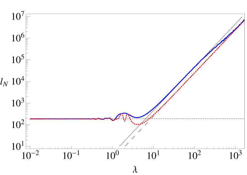
We first consider stacks having refractive index and thickness disorder, with and . Shown in Fig. 2 are transmission spectra for a M-stack of layers and a H-stack of length . There are two major differences between the results for these two types of samples: first, in the localized regime (), the transmission length of the M-stack exceeds or coincides with that of the H-stack; second, in the long wavelength region, the plot of the transmission length of the M-stack exhibits a pronounced bend, or kink, in the interval , while there is no such feature in the H-stack results. These two types of behaviour are discussed in more detail below.
IV.1.1 Mixed stacks
The weak scattering approximation (WSA) of Eq. (18) is an excellent method by which to calculate the transmission length for M-stacks. This is seen in Fig. 2 where the curves obtained by numerical simulations and by the WSA are indistinguishable (solid line). The characteristic wavelengths (40) of this mixed stack are and . Therefore, the transmission length describes the localization properties of a random sample in the region , whereas longer wavelengths, , correspond to the ballistic regime. The crossover from the localized to the ballistic regime demonstrates the kink-type behaviour that occurs within the region . The short and long wavelength behaviour of the transmission length is also in excellent agreement with the calculated asymptotics in both regimes.
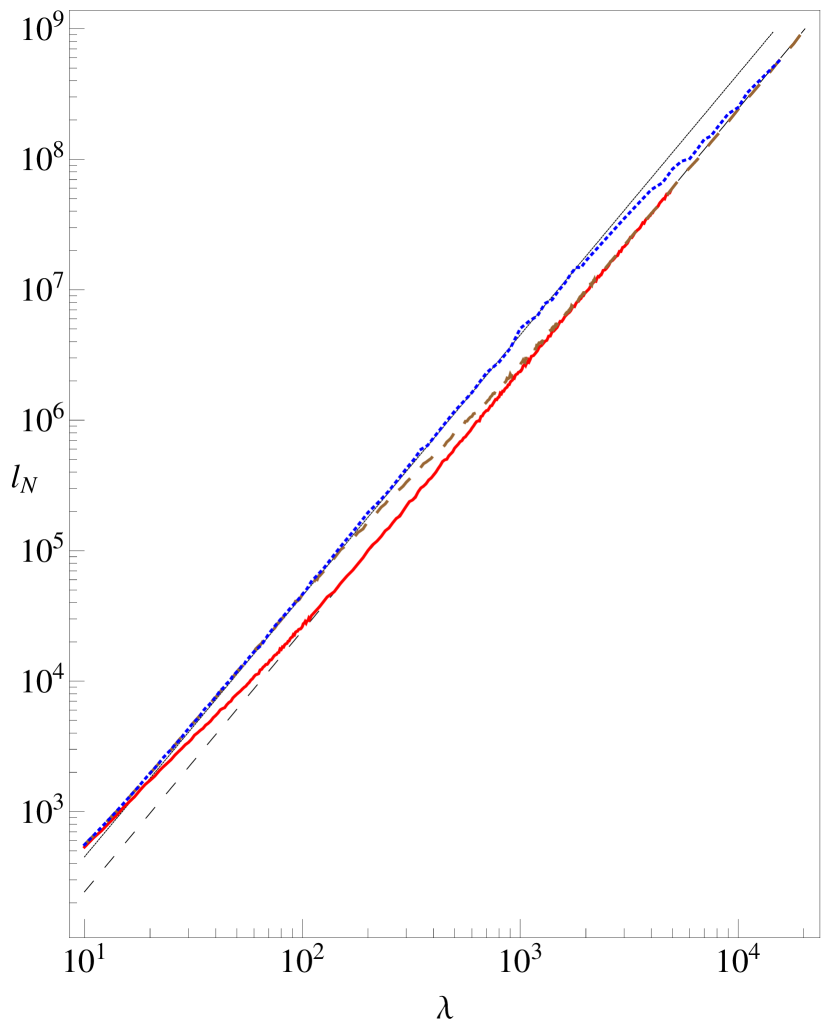
To analyze the long wavelength region () more carefully, we plot in Fig. 3 the transmission lengths of M-stacks of three different sizes, In all cases, there is excellent agreement between the simulations and the WSA predictions. The characteristic wavelengths for are and , while for they are and , and we see that the observed crossover regions are bounded exactly by these characteristic wavelengths in all three cases.
To confirm the ballistic nature of the transmission in the region , we plot in Fig. 4(a) the logarithm of the mean value of the reflectance for the same three stack sizes as a function of the logarithm of the wavelength. In all cases, the plots exhibit a linear dependence in the ballistic regime, which is bounded from below by the crossover wavelength . The straight lines are calculated from Eq. (35) and confirm that the reflection coefficient in the mixed stack is proportional to the stack length. Within the localized region , the reflection coefficient is close to unity in all three cases.
The behaviour of the transmission length is illustrated by the phase diagram in the plane shown in Fig. 4(b). The two slanted lines and separate the plane into three parts corresponding to the localization (I), the crossover region (II) and the ballistic region (III). The intersections of these lines with the horizontal lines , , and define the characteristic wavelengths and for the three stack sizes considered here. It is easy to see that these wavelengths, determined with the aid of the phase diagram, perfectly bound the crossover regions in both Fig. 3 and Fig. 4(a).
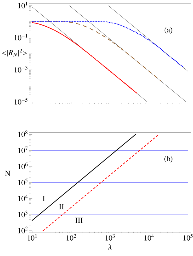
(b) Phase diagram of M-stacks. The thick solid line corresponds to a stack size equal to the localization length. The dashed line corresponds to a stack size equal to the crossover length. The localized, crossover and ballistic regimes occur in regions I, II, and III respectively.
Until now, we have dealt only with the transmission length , which was defined through an average value. However, more detailed information can be obtained from the transmission length for a single realization, defined by the equation
| (63) |
In the localized regime, for a sufficiently long (i.e., ) M-stack, the transmission length for a single realization is practically non-random and coincides with , while in the ballistic region it fluctuates. The data displayed in Fig. 5) enables us to estimate the difference between the transmission length (solid line) and the transmission length for a single randomly chosen realization (dashed line), and the scale of the corresponding fluctuations. Both curves are smooth, coincide in the localized region, and differ noticeably in the ballistic regime. The separate discrete points in Fig. 5 present the values of the transmission length calculated for different randomly chosen realizations. It is evident that fluctuations in the ballistic region become more pronounced with increasing wavelength.
IV.1.2 Homogeneous stacks
The absence of any kink in the H-stack transmission length spectrum in Fig. 2 follows from Sec. III.2.3 in which it was shown that the crossover to the far ballistic regime occurs at the wavelength (45). For , this is of the order of and so the kink does not appear.
In order to study the crossover, we plot in Fig. 6 the transmission lengths of H-stacks with and over the wavelength range extended up to . As for the M-stack, the simulation results for H-stacks cannot be distinguished from those of the WSA (42). The transition from the localized to the near ballistic regime occurs without any change in the analytical dependence of transmission length, in complete agreement with the results of Sec. III.2.3. The crossover from the near to the far ballistic regime is accompanied by a change in the analytical dependence that occurs at , which for these stacks is of the order of and respectively. The crossover is accompanied by prominent oscillations described by Eq. (52). Finally, we note that the vertical displacement between the moderately long and extremely long wavelength ballistic asymptotes does not depend on wavelength, but grows with the size of the stack, according to the law
| (64) |
which stems from Eq. (50).
To study the ballistic transmission regime in the region more closely, we plot in the upper panel of Fig. 7(a) (on a logarithmic scale) the mean value of the reflection coefficient for the same two stack sizes. That part of each plot which presents the ballistic propagation comprises two linear asymptotes of the form , corresponding to different values of the constant, one applicable in the near ballistic region and the other in the far ballistic region . The difference between the values of these two constants corresponds precisely with the right hand side of Eq. (64), with the far long wavelength asymptotic given by the second term in Eq. (52). Within the localized regime the reflectance is almost unity in all three cases.

By analogy with M-stacks, the behaviour of the transmission length in the plane is illustrated by the phase diagram displayed in the lower panel of Fig. 7. Two slanted lines and divide the plane into three parts corresponding to the localization regime (I), the crossover regime (II) and the ballistic regime (III). The wavelength, at which these lines intersect the horizontal lines corresponding to the stack lengths, , and , defines the characteristic wavelengths (III.2.3) for each stack size. From Fig. 7(b), it follows that the separation between them grows with increasing size in accordance with Eq. (64). It is easy to see that the wavelengths determined from the phase diagram perfectly bound the near ballistic region in both Fig. 6 and Fig. 7(a).
We now consider the transmission length for a H-stack computed using a single realization. For extremely long stacks (), the transmission length becomes practically non-random, not only within the localized region (as is the case for M-stacks) but also in the far ballistic region because of the self-averaging nature of the effective dielectric constant (58). For less long stacks, however, also fluctuates in the far ballistic region. To demonstrate this, we have plotted in Fig. 8 the transmission length (solid line) and the transmission length for a single randomly chosen realization (dashed line). It is evident that, in contrast to the results for the M-stack, the H-stack single realization transmission length in the near ballistic region is a complicated and irregular function, similar to the well known “magneto fingerprints” of magneto-conductance of a disordered sample in the weak localization regime Altshu . In the far ballistic region, these fluctuations are moderated since they vanish in the limit as . To support this statement, we display in Fig. 8 the set of separate discrete points, each of them presenting calculated for a different randomly chosen realization.
In summary, we note that the results of Sec. IV.1 show excellent agreement between the numerical simulations and the analytical predictions of the weak scattering approximation of Sec. III. Moreover, even for the case of an H-stack of length and strong disorder, and , the results of direct simulation and those of the WSA analysis coincide completely in the long wavelength region and differ by only a few percent in the short wave region where the scattering is certainly not weak. This is because the perturbation approach based on Eqs. (11), (12) is related not to the calculated quantities but to the equations they satisfy.
IV.2 Refractive-index disorder
IV.2.1 Suppression of localization
Here, we present results for stacks with only refractive index disorder (RID), with . For H-stacks, the transmission length demonstrates qualitatively and quantitatively the same behaviour as was observed in the presence of both refractive index and thickness disorder. Corresponding formulae for the transmission, localization, and ballistic lengths can be obtained from the general case by taking the limit as .
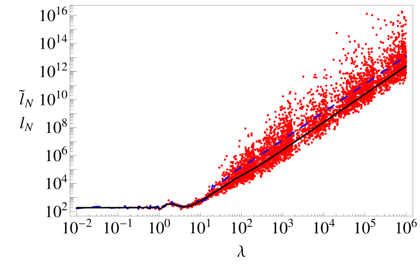
In the case of M-stacks, however, the situation changes markedly. While in the short wavelength region and in the ballistic regime the numerical results are still in a excellent agreement with the predictions of the weak scattering approximation, the WSA fails in the long wavelength part of the localization regime. This discrepancy manifests itself also for short stacks, in which the localization regime in the long wave region is absent. In Fig. 9 we present the transmission length spectrum for a M-stack of layers, showing that, for , the numerical results for the transmission lengths of M-stacks differ by an order of magnitude from those predicted by the WSA analysis, and also those observed for the corresponding H-stacks.
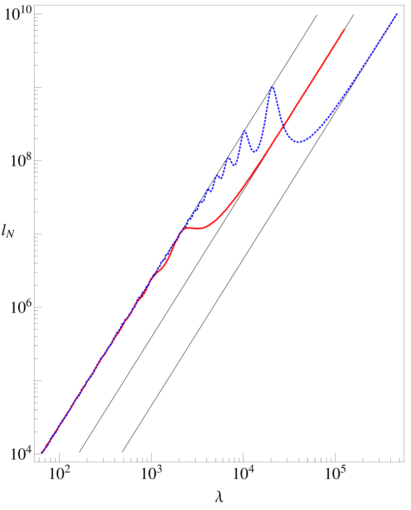
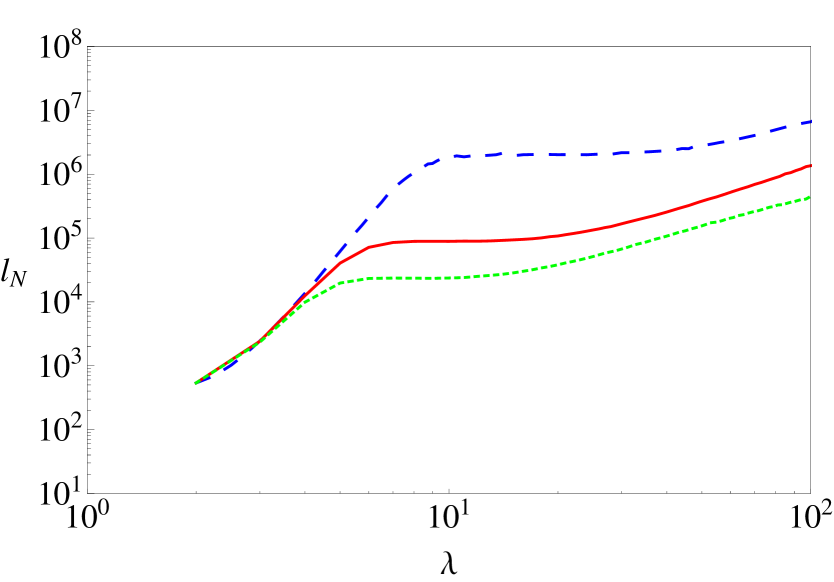
For longer stacks, the differences in the transmission length spectra exhibited by M-stacks and H-stacks becomes much more pronounced. In Fig. 10, we plot transmission length spectra for different values of the M-stack length with (using realizations), (using realizations) and layers (using only a single realization), with the dashed-dotted straight line in Fig. 10 showing the long wavelength ballistic asymptote (33). In the moderately long wavelength region corresponding to the localization regime, the transmission length coincides with the localization length . It exceeds the H-stack localization length by a few orders of magnitude and is characterized by a completely different wavelength dependence. This substantial suppression of localization was revealed in our earlier paper we where the localization length was reported to be proportional to , in contrast to the classical dependence (36) that is observed for H-stacks, and which is also valid for M-stacks with both refractive index and thickness disorder. The reason for this difference is the lack of phase accumulation caused by the phase cancelation in alternating layers of equal thicknesses.
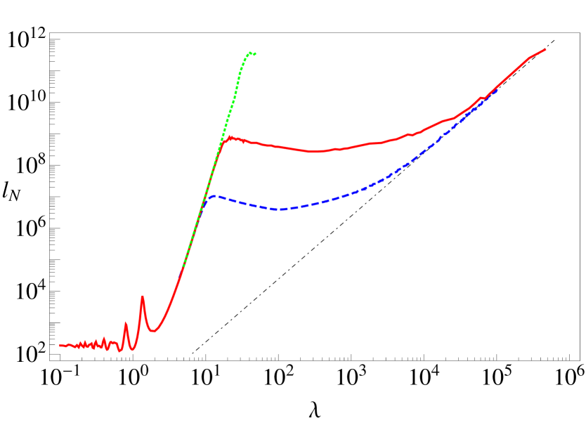
To study this behaviour in more detail, we generate a least squares fit to the transmission length data. Respectively, for , , and layers, the best fits are , and , indicating that the asymptotic form for the localization length differs from a pure power law, and perhaps is described by a non-analytic dependence.
In the crossover part of the long-wave region where , the transmission length of M-stacks also differs essentially from that for H-stacks. Moreover, the width of the crossover region on the axis remains of the same order of magnitude, although on the axis it grows for to four orders of magnitude, being much wider for longer stacks. In the long wavelength region corresponding to the ballistic regime, the transmission length of the RID M-stack coincides with that of RID H-stack.
IV.2.2 Transmission resonances
An important signature of the localization regime is the presence of transmission resonances (see, for example, Refs. Lifshits ; Azbel ; Bliokh-2 ), which appears in sufficiently long, open systems and which are a “fingerprint” of a given realization of disorder. These resonances are responsible for the difference between two quantities that characterize the transmission, namely and . The former reflects the properties of a typical realization, while the main contribution to the latter is generated by a small number of almost transparent realizations associated with the transmission resonances.
The natural characteristic of the transmission resonances is the ratio of the two quantities mentioned above:
In the absence of resonances, this value is close to unity, while in the localization regime . In particular, in the high-energy part of the spectrum of a disordered system with Gaussian white-noise potential, this ratio takes the value LGP .
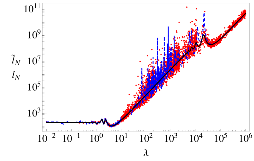
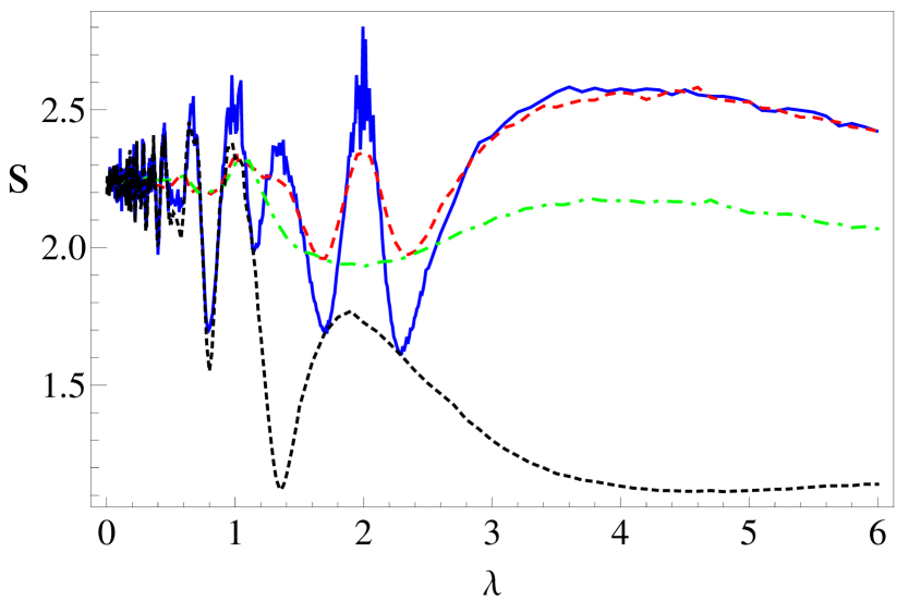
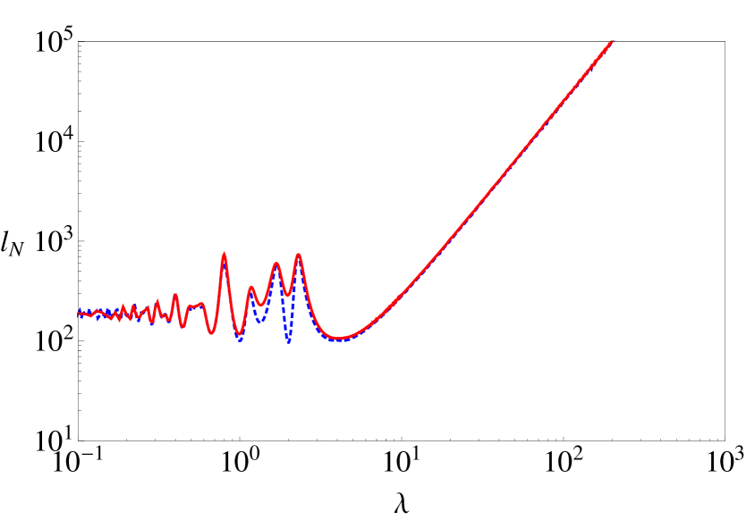
In Fig. 11, we plot the ratio as a function of the wavelength for RID M- and H-stacks and for the corresponding stacks with thickness disorder. In all cases, the stack length is and it is evident that for the RID M-stack , i.e.. the stack length is too short for the localization regime to be realized. In other three cases, however, , which means that the localization takes place even in a comparatively short stack.
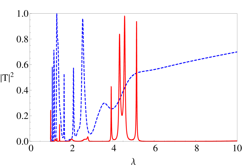
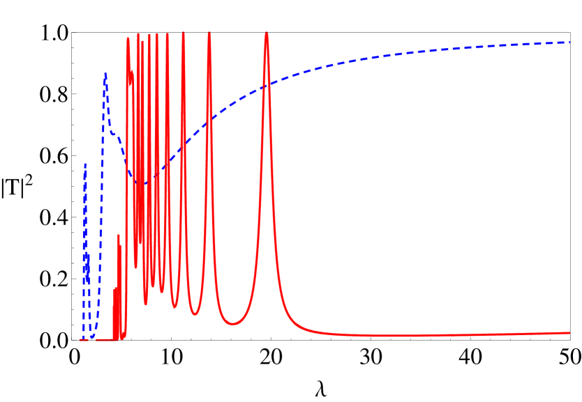
Thus, there are two ways in which to introduce transmission resonances. The first is to increase the length of the stack. Fig. 12 displays the RID M-stack transmittance for a single realization as a function of for two lengths: (solid line) and (dotted line). It is readily seen that while there are no resonances in the shorter stacks, they do appear for the longer sample. The second way to generate transmission resonances is to introduce thickness disorder. To demonstrate this, we plot in Fig. 13 the transmittance of a single M-stack with both thickness and refractive index disorder. It clearly shows that while the RID M-stack is too short to exhibit transmission resonances at , resonances do emerge at longer wavelengths for the M-stack with thickness disorder.
IV.2.3 Effects of the thickness disorder and uncorrelated paring
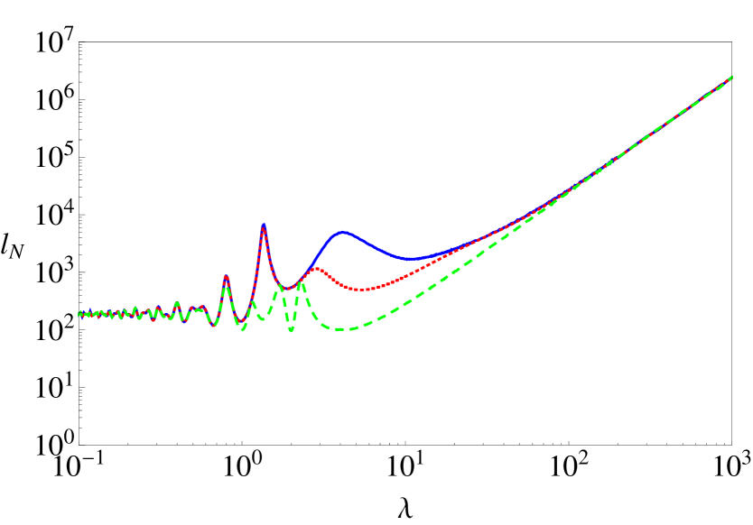
Here, we analyze the effect of thickness disorder on the -anomaly — that is the dependence of the transmission length. In Fig. 14, we plot the transmission length for an M-stack with fixed refractive index disorder ( for various values of the thickness disorder. It is evident that the transmission length changes from to the classical dependence as the thickness disorder increases from (top curve) to (bottom curve). In all cases, the number of layers is longer than the transmission length, guaranteeing that Fig. 14 represents the genuine localization length .
We have also found that the anomalous dependence (or with higher power) is extremely sensitive to the alternation of left- and right-handed layers. To demonstrate this, we consider an M-stack of length in which each subsequent layer is chosen with equal probability to be either right- or left-handed. Figure 15 shows the transmission length spectrum for this case, which is almost the same for both the H-stacks and M-stacks. The only difference is a fairly modest suppression of localization, which occurs within the wavelength interval . This result confirms that it is the additional correlation between left-handed and right-handed layers in the alternating stack which is responsible for the suppression of localization.
IV.3 Effects of losses
In this section, we study the transmission through layered media with absorption, which is characteristic of real metamaterials. In this case, the exponential decay of the field is due to both Anderson localization and absorption FrePusYur ; Asatrian2 , and in some limiting cases, it is possible to distinguish between these contributions.
For an M-stack with weak fluctuations of the refractive index, weak thickness disorder and weak absorbtion, the WSA theory in the limits of short or long waves leads to the well-known formula
where is the disorder-induced transmission length in the absence of absorption, and the absorption length is
| (65) |
For short wavelengths, is a constant given by Eqs (29), (33) and (36), while for long wavelengths, in either the localized or ballistic regimes, its contribution is proportional to and thus is negligibly small in comparison with the contribution due to losses, which is always proportional to . Accordingly, at both short and long wavelengths, the attenuation length coincides with the absorption length (65), with disorder contributing significantly to the attenuation length only in some intermediate wavelength region, provided that the absorption is sufficiently small.
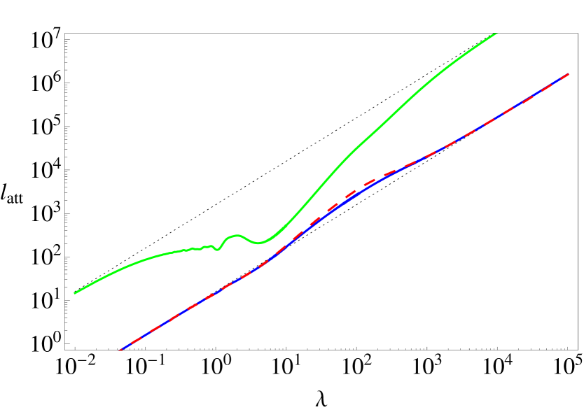
The results of the numerical calculations shown in Fig. 16 completely confirm the theoretical predictions presented above. For weak absorption , the direct simulation and WSA theory give exactly the same result (solid curve in Fig. 16). Over a reasonably wide wavelength range, , disorder contributes significantly to the attenuation. For such a stack, the characteristic wavelengths are and , implying that the contribution of disorder is significant in all regions, from the short wavelength part of the localized regime to the long wavelength ballistic region. Due to the losses, however, there are fewer oscillations evident in the transmission length spectrum than in the lossless case of Fig. 2.
For stronger absorption, , the wavelength range, over which disorder contributes to the attenuation is reduced, as well as the relative value of the contribution itself. The agreement between the numerical simulations and the WSA calculations is reasonable.
V Conclusions
We have studied the transmission and localization of classical waves in one-dimensional disordered structures composed of alternating layers of left- and right-handed materials (M-stacks) and have compared this to the transport in homogeneous structures composed of different layers of the same material (H-stacks). For weakly scattering layers and general disorder, where both refractive index and thickness of each layer is random, we have developed an effective analytical approach, which has enabled us to calculate the transmission length over a wide range of input parameters and to describe transmission through M- and H-stacks in a unified way. All theoretical predictions are in excellent agreement with the results of direct numerical simulations.
There are remarkable distinctions between the transmission and localization properties of the two types of stacks. When both types of disorder (refractive index and layer thickness) are present, the transmission length of a H-stack in the localized regime coincides with the reciprocal of the Lyapunov exponent, while for M-stacks these two quantities differ by a numerical prefactor. This is quite surprising and, to the best of our knowledge, it is the first time that a system where such a difference exists has been discovered.
It is shown that the stacks of M- and H-type manifest quite different behaviour of the transmission length as a function of wavelength. This difference is most pronounced in the long wavelength region. In the localized regime, stacks of both types are strongly disordered and reflect the incident wave almost entirely. In the ballistic regime, where stacks are almost transparent, the transport properties of H-stacks and M-stacks are markedly different. H-stacks, over the moderately long wavelength ballistic region, and M-stacks, over the entire long wavelength region, are weakly scattering disordered structures. In the extremely long wavelength ballistic region, the H-stack becomes effectively uniform — a regime which is absent for M-stacks because of the intrinsic non-uniformity caused by the alternating nature of the structure. The crossover regions between different regimes are comparatively narrow.
The transmission length for a single realization is non-random in the localized regime for both types of stacks. It fluctuates strongly over the entire ballistic region for M-stacks and in the near ballistic regime for H-stacks. In the far long wave region for H-stacks, the fluctuations apparent in the transmission length are moderate and decrease with increasing stack length. In the case of M-stacks, the transition from the localized to the ballistic regime is accompanied by a change in the wavelength dependence of the transmission length. In contrast, for H-stacks, the corresponding change occurs in the vicinity of the transition from the near to the far ballistic regime. Again, the crossover regions between the different regimes are comparatively narrow.
In M-stacks with only refractive-index disorder, Anderson localization is substantially suppressed, and the localization length grows with increasing wavelength much faster than the classical square law dependence. The crossover region becomes significantly wider, and transmission resonances occur in much longer stacks than in the corresponding H-stacks.
The effects of absorption on the one-dimensional transport and localization have also been studied, both analytically and numerically. In particular, it has been shown that the crossover region is particularly sensitive to losses, so that even small absorption noticeably suppresses the oscillations of the transmission length in the frequency domain.
VI Acknowledgments
This work was supported by the Australian Research Council through
the Discovery and Centres of Excellence programs, and also by the Israel
Science Foundation (Grant # 944/05). We thank L. Pastur, K. Bliokh and Yu.
Bliokh for useful discussions. We also acknowledge the provision of
computing facilities through NCI (National Computational Infrastructure) and Intersect in Australia.
*
Appendix A Uniform distribution of fluctuations
If the fluctuations and are uniformly distributed in the intervals and respectively, and absorption is the same in all slabs (), the transmission, localization, and ballistic lengths given by Eqs. (22)-(26) can be calculated explicitly in the weak scattering approximation. The results are:
| (66) | |||||
| (67) | |||||
| (68) | |||||
Here,
where is obtained from by the replacement of by , and is the exponential integral given by
References
- (1) V. G. Veselago, Sov. Phys. Usp. 10, 509 (1968).
- (2) J. B. Pendry, Phys. Rev. Lett. 85, 3966 (2000).
- (3) P. Marcos, C.M. Soukoulis, Wave propagation from electrons to photonic crystals and left-handed materials, (Princeton University Press, Princeton, 2008).
- (4) K. Yu. Bliokh, and Yu. P. Bliokh, Physics - Uspekhi 47, 393 (2004) [Usp. Fiz. Nauk 174, 439 (2004)].
- (5) C. Caloz and T. Ito, Proceedings of IEEE 93, 1744 (2005).
- (6) V. M. Shalaev, Nature Photonics 1, 41 (2007).
- (7) D. Schurig, J. Mock, B. Justice, S. Cummer, J. Pendry, A. Starr, and D. Smith, Science 314, 977 (2006).
- (8) J. Kstel and M. Fleischhauer, Phys. Rev. A 71, 011804(R) (2005).
- (9) Y. Yang, J. Xu, H. Chen, and S. Zhu, Phys. Rev. Lett. 100, 043601 (2008).
- (10) L. G. Wang, H. Chen, and S.-Y. Zhu, Phys. Rev. B 70, 245102 (2004).
- (11) M. V. Gorkunov, S. A. Gredeskul, I. V. Shadrivov, and Yu. S. Kivshar, Phys. Rev. E 73, 056605 (2006).
- (12) P. W. Anderson, Phys. Rev. 109, 1492 (1958).
- (13) S. John, Phys. Rev. Lett., 53, 2169 (1984).
- (14) I. M. Lifshits, S. A. Gredeskul, and L. A. Pastur, Introduction to the Theory of Disordered Systems (Wiley, New York 1987).
- (15) P. Sheng, Scattering and localization of classical waves in random media (Singapore: World Scientific 1991).
- (16) V. D. Freilikher and S.A. Gredeskul, Progress in Optics 30, 137 (1992).
- (17) S. A. Gredeskul, A. V. Marchenko, and L. A. Pastur, Surveys in Applied Mathematics, v. 2 (Plenum Press, New York 1995), p. 63.
- (18) P. Sheng, Introduction to Wave Scattering, Localization, and Mesoscopic Phenomena (Springer-Verlag, Heidelberg, 2006).
- (19) N. Mott and Twose, Adv. Phys. 10, 107 (1961).
- (20) F. M. Israilev, N. M. Makarov, E. J. Torres-Herrera, arXiv:0911.0966v1 [cond-mat.mes-hall], 5 Nov. 2009.
- (21) Y. Dong and X. Zhang, Phys. Lett. A 359, 542 (2006).
- (22) A. A. Asatryan, L. C. Botten, M. A. Byrne, V. D. Freilikher, S. A. Gredeskul, I. V. Shadrivov, R. C. McPhedran, and Yu. S. Kivshar, Phys. Rev. Lett. 99, 193902 (2007).
- (23) V. Baluni and J. Willemsen, Phys. Rev. A 31, 3358 (1985).
- (24) E. M. Nascimento, F. A. B. F. de Moura, and M. L. Lyra, Optics Express 16, 6860 (2008).
- (25) P. Han, C. T. Chan, and Z. Q. Zhang, Phys. Rev. B 77, 115332 (2008).
- (26) C. Martijn de Sterke, and R. C. McPhedran, Phys. Rev. B 47, 7780 (1993).
- (27) A. A. Asatryan, N. A. Nicorovici, L. C. Botten, C. M. de Sterke, P. A. Robinson, and R. C. McPhedran, Phys. Rev. B 57, 13535 (1998).
- (28) G. A. Luna-Acosta, F. M. Izrailev, N. M. Makarov, U. Kuhl, and H.-J. Stckmann, Phys. Rev. B 80, 115112 (2009).
- (29) S. M. Rytov, Yu. A. Kravtsov, and V. I. Tatarskii, Principles of Statistical Radiophysics (Springer, Berlin, 1987).
- (30) V.D. Freilikher, B.A. Liansky, I.V. Yurkevich, A.A. Maradudin, A.R. McGurn, Phys. Rev. E 51, 6301 (1995).
- (31) A. A. Asatryan, P. A. Robinson, L. C. Botten, R. C. McPhedran, N. A. Nicorovici and C. Martijn de Sterke, Phys. Rev. E 60, 6118 (1999).
- (32) B. L. Altshuler, A. G. Aronov, and B. Z. Spivak, JETP Lett. 32, 94 (1981).
- (33) I. M. Lifshitz and V. Ya. Kirpichenkov, Sov. Phys. JETP 50, 499 (1979) [Zh. Eksp. Teor. Fiz. 77, 989 (1979)].
- (34) M. Ya. Azbel and P. Soven, Phys. Rev. B 27, 831 (1983).
- (35) K. Yu. Bliokh, Yu. P. Bliokh, V. Freilikher, S. Savelïev, and F. Nori, Rev. Mod. Phys. 80, 1201 (2008).
- (36) V. Freilikher, M. Pustilnik, and I. Yurkevich, Phys. Rev. B 50, 6017 (1994).