arXiv:0912.0361 [hep-ph]

Abstract

This lecture discusses the Higgs boson sector of the SM and the MSSM, including their connection to electroweak precision physics and the searches for SM and SUSY Higgs bosons at the LHC.

Chapter 1 Higgs and Electroweak Physics

Sven Heinemeyer
Instituto de Física de Cantabria (CSIC), Santander, Spain

1 Introduction

A major goal of the particle physics program at the high energy frontier, currently being pursued at the Fermilab Tevatron collider and soon to be taken up by the CERN Large Hadron Collider (LHC), is to unravel the nature of electroweak symmetry breaking. While the existence of the massive electroweak gauge bosons ($W^{\pm},Z$), together with the successful description of their behavior by non-abelian gauge theory, requires some form of electroweak symmetry breaking to be present in nature, the underlying dynamics is not known yet. An appealing theoretical suggestion for such dynamics is the Higgs mechanism [1], which implies the existence of one or more Higgs bosons (depending on the specific model considered). Therefore, the search for Higgs bosons is a major cornerstone in the physics programs of past, present and future high energy colliders.

Many theoretical models employing the Higgs mechanism in order to account for electroweak symmetry breaking have been studied in the literature, of which the most popular ones are the Standard Model (SM) [4] and the Minimal Supersymmetric Standard Model (MSSM) [5]. Within the SM, the Higgs boson is the last undiscovered particle, whereas the MSSM has a richer Higgs sector, containing three neutral and two charged Higgs bosons. Among alternative theoretical models beyond the SM and the MSSM, the most prominent are the Two Higgs Doublet Model (THDM) [6], non-minimal supersymmetric extensions of the SM (e.g. extensions of the MSSM by an extra singlet superfield [7]), little Higgs models [8] and models with more than three spatial dimensions [9].

We will discuss the Higgs boson sector in the SM and the MSSM. This includes their connection to electroweak precision physics and the searches for the SM and supersymmetric (SUSY) Higgs bosons at the LHC. While the LHC will discover a SM Higgs boson and, in case that the MSSM is realized in nature, almost certainly also one or more SUSY Higgs bosons, a “cleaner” experimental environment, such as at the ILC, will be needed to measure all the Higgs boson characteristics [10, 11].

2 The SM and the Higgs

2.1 Higgs: Why and How?

We start with looking at one of the most simple Lagrangians, the one of QED:

$${\cal L}_{\rm QED} =-\frac{1}{4}F_{\mu\nu}F^{\mu\nu}+\bar{\psi}(i\gamma^{\mu}D_{\mu}-m)\psi~{}.$$ (1)

Here $D_{\mu}$ denotes the covariant derivative

$$D_{\mu} =\partial_{\mu}+i\,e\,A_{\mu}~{}.$$ (2)

$\psi$ is the electron spinor, and $A_{\mu}$ is the photon vector field. The QED Lagrangian is invariant under the local $U(1)$ gauge symmetry,

$$\psi \to e^{-i\alpha(x)}\psi~{},$$ (3)

$$A_{\mu} \to A_{\mu}+\frac{1}{e}\partial_{\mu}\alpha(x)~{}.$$ (4)

Introducing a mass term for the photon,

$${\cal L}_{\rm photon~{}mass} =\frac{1}{2}m_{A}^{2}A_{\mu}A^{\mu}~{},$$ (5)

however, is not gauge-invariant. Applying Eq. (4) yields

$$\frac{1}{2}m_{A}^{2}A_{\mu}A^{\mu} \to\frac{1}{2}m_{A}^{2}\left[A_{\mu}A^{\mu}+\frac{2}{e}A^{\mu}\partial_{\mu}\alpha+\frac{1}{e^{2}}\partial_{\mu}\alpha\,\partial^{\mu}\alpha\right]~{}.$$ (6)

A way out is the Higgs mechanism [1]. The simplest implementation uses one elementary complex scalar Higgs field $\Phi$ that has a vacuum expectation value $v$ (vev) that is constant in space and time. The Lagrangian of the new Higgs field reads

$${\cal L}_{\Phi} ={\cal L}_{\Phi,{\rm kin}}+{\cal L}_{\Phi,{\rm pot}}$$ (7)

with

$${\cal L}_{\Phi,{\rm kin}} =(D_{\mu}\Phi)^{*}\,(D^{\mu}\Phi)~{},$$ (8)

$$-{\cal L}_{\Phi,{\rm pot}} =V(\Phi)=\mu^{2}|\Phi|^{2}+\lambda|\Phi|^{4}~{}.$$ (9)

Here $\lambda$ has to be chosen positive to have a potential bounded from below. $\mu^{2}$ can be either positive or negative, where we will see that $\mu^{2}<0$ yields the desired vev, as will be shown below. The complex scalar field $\Phi$ can be parametrized by two real scalar fields $\phi$ and $\eta$,

$$\Phi(x) =\frac{1}{\sqrt{2}}\phi(x)e^{i\eta(x)}~{},$$ (10)

yielding

$$V(\phi) =\frac{\mu^{2}}{2}\phi^{2}+\frac{\lambda}{4}\phi^{4}~{}.$$ (11)

Minimizing the potential one finds

$$\frac{{\rm d}V}{{\rm d}\phi}_{\big{|}\phi=\phi_{0}} =\mu^{2}\phi_{0}+\lambda\phi_{0}^{3}\stackrel{{\scriptstyle!}}{{=}}0~{}.$$ (12)

Only for $\mu^{2}<0$ this yields the desired non-trivial solution

$$\phi_{0} =\sqrt{\frac{-\mu^{2}}{\lambda}}\left(=\langle\phi\rangle=:v\right)~{}.$$ (13)

The picture simplifies more by going to the “unitary gauge”, $\alpha(x)=-\eta(x)/v$, which yields a real-valued $\Phi$ everywhere. The kinetic term now reads

$$(D_{\mu}\Phi)^{*}\,(D^{\mu}\Phi) \to\frac{1}{2}(\partial_{\mu}\phi)^{2}+\frac{1}{2}e^{2}q^{2}\phi^{2}A_{\mu}A^{\mu}~{},$$ (14)

where $q$ is the charge of the Higgs field, which can now be expanded around its vev,

$$\phi(x) =v\;+\;H(x)~{}.$$ (15)

The remaining degree of freedom, $H(x)$ is a real scalar boson, the Higgs boson. The Higgs boson mass and self-interactions are obtained by inserting Eq. (15) into the Lagrangian (neglecting a constant term),

$$-{\cal L}_{\rm Higgs} =\frac{1}{2}m_{H}^{2}H^{2}+\frac{\kappa}{3!}H^{3}+\frac{\xi}{4!}H^{4}~{},$$ (16)

with

$$m_{H}^{2}=2\lambda v^{2},\quad\kappa=3\frac{m_{H}^{2}}{v},\quad\xi=3\frac{m_{H}^{2}}{v^{2}}~{}.$$ (17)

Similarly, Eq. (15) can be inserted in Eq. (14), yielding (neglecting the kinetic term for $\phi$),

$${\cal L}_{\rm Higgs-photon} =\frac{1}{2}m_{A}^{2}A_{\mu}A^{\mu}+e^{2}q^{2}vHA_{\mu}A^{\mu}+\frac{1}{2}e^{2}q^{2}H^{2}A_{\mu}A^{\mu}$$ (18)

where the second and third term describe the interaction between the photon and one or two Higgs bosons, respectively, and the first term is the photon mass,

$$m_{A}^{2} =e^{2}q^{2}v^{2}~{}.$$ (19)

Another important feature can be observed: the coupling of the photon to the Higgs is proportional to its own mass squared.

Similarly a gauge invariant Lagrangian can be defined to give mass to the chiral fermion $\psi=(\psi_{L},\psi_{R})^{T}$,

$${\cal L}_{\rm fermion~{}mass} =y_{\psi}\psi_{L}^{\dagger}\,\Phi\,\psi_{R}+{\rm c.c.}~{},$$ (20)

where $y_{\psi}$ denotes the dimensionless Yukawa coupling. Inserting $\Phi(x)=(v+H(x))/\sqrt{2}$ one finds

$${\cal L}_{\rm fermion~{}mass} =m_{\psi}\psi_{L}^{\dagger}\psi_{R}+\frac{m_{\psi}}{v}H\,\psi_{L}^{\dagger}\psi_{R}+{\rm c.c.}~{},$$ (21)

with

$$m_{\psi} =y_{\psi}\frac{v}{\sqrt{2}}~{}.$$ (22)

Again the important feature can be observed: by construction the coupling of the fermion to the Higgs boson is proportional to its own mass $m_{\psi}$.

The “creation” of a mass term can be viewed from a different angle. The interaction of the gauge field or the fermion field with the scalar background field, i.e. the vev, shift the masses of these fields from zero to non-zero values. This is shown graphically in Figure 1 for the gauge boson (a) and the fermion (b) field.

Figure 1: Generation of a gauge boson mass (a) and a fermion mass (b) via the interaction with the vev of the Higgs field.

The shift in the propagators reads (with $p$ being the external momentum and $g=eq$ in Eq. (19)):

$$(a)\; \frac{1}{p^{2}}\;\to\;\frac{1}{p^{2}}+\sum_{k=1}^{\infty}\frac{1}{p^{2}}\left[\left(\frac{gv}{2}\right)\frac{1}{p^{2}}\right]^{k} =\frac{1}{p^{2}-m_{V}^{2}}{\rm~{}with~{}}m_{V}^{2}=g^{2}\frac{v^{2}}{4}~{},$$ (23)

$$(b)\; \frac{1}{\makebox[0.86108pt][l]{$p$}/}\;\to\;\frac{1}{\makebox[0.86108pt][l]{$p$}/}+\sum_{k=1}^{\infty}\frac{1}{\makebox[0.86108pt][l]{$p$}/}\left[\left(\frac{y_{\psi}v}{2}\right)\frac{1}{\makebox[0.86108pt][l]{$p$}/}\right]^{k} =\frac{1}{\makebox[0.86108pt][l]{$p$}/-m_{\psi}}{\rm~{}with~{}}m_{\psi}=y_{\psi}\frac{v}{\sqrt{2}}~{}.$$ (24)

2.2 SM Higgs Theory

We now turn to the electroweak sector of the SM, which is described by the gauge symmetry $SU(2)_{L}\times U(1)_{Y}$. The bosonic part of the Lagrangian is given by

$${\cal L}_{\rm bos} =-\frac{1}{4}B_{\mu\nu}B^{\mu\nu}-\frac{1}{4}W_{\mu\nu}^{a}W^{\mu\nu}_{a}+|D_{\mu}\Phi|^{2}-V(\Phi),$$ (25)

$$V(\Phi) =\mu^{2}|\Phi|^{2}+\lambda|\Phi|^{4}~{}.$$ (26)

$\Phi$ is a complex scalar doublet with charges $(2,1)$ under the SM gauge groups,

$$\Phi =\left(\begin{array}[]{c}\phi^{+}\\ \phi^{0}\end{array}\right)~{},$$ (29)

and the electric charge is given by $Q=T^{3}+\frac{1}{2}Y$, where $T^{3}$ the third component of the weak isospin. We furthermore have

$$D_{\mu} =\partial_{\mu}+ig\frac{\tau^{a}}{2}W_{\mu\,a}+ig^{\prime}\frac{Y}{2}B_{\mu}~{},$$ (30)

$$B_{\mu\nu} =\partial_{\mu}B_{\nu}-\partial_{\nu}B_{\mu}~{},$$ (31)

$$W_{\mu\nu}^{a} =\partial_{\mu}W_{\nu}^{a}-\partial_{\nu}W_{\mu}^{a}-gf^{abc}W_{\mu\,b}W_{\nu\,c}~{}.$$ (32)

$g$ and $g^{\prime}$ are the $SU(2)_{L}$ and $U(1)_{Y}$ gauge couplings, respectively, $\tau^{a}$ are the Pauli matrices, and $f^{abc}$ are the $SU(2)$ structure constants.

Choosing $\mu^{2}<0$ the minimum of the Higgs potential is found at

$$\langle\Phi\rangle =\frac{1}{\sqrt{2}}\left(\begin{array}[]{c}0\\ v\end{array}\right)\quad{\rm with}\quad v:=\sqrt{\frac{-\mu^{2}}{\lambda}}~{}.$$ (35)

$\Phi(x)$ can now be expressed through the vev, the Higgs boson and three Goldstone bosons $\phi_{1,2,3}$,

$$\Phi(x) =\frac{1}{\sqrt{2}}\left(\begin{array}[]{c}\phi_{1}(x)+i\phi_{2}(x)\\ v+H(x)+i\phi_{3}(x)\end{array}\right)~{}.$$ (38)

Diagonalizing the mass matrices of the gauge bosons, one finds that the three massless Goldstone bosons are absorbed as longitudinal components of the three massive gauge bosons, $W_{\mu}^{\pm},Z_{\mu}$, while the photon $A_{\mu}$ remains massless,

$$W_{\mu}^{\pm} =\frac{1}{\sqrt{2}}\left(W_{\mu}^{1}\mp iW_{\mu}^{2}\right)~{},$$ (39)

$$Z_{\mu} =c_{\mathrm{w}}W_{\mu}^{3}-s_{\mathrm{w}}B_{\mu}~{},$$ (40)

$$A_{\mu} =s_{\mathrm{w}}W_{\mu}^{3}+c_{\mathrm{w}}B_{\mu}~{}.$$ (41)

Here we have introduced the weak mixing angle $\theta_{W}=\arctan(g^{\prime}/g)$, and $s_{\mathrm{w}}:=\sin\theta_{W}$, $c_{\mathrm{w}}:=\cos\theta_{W}$. The Higgs-gauge boson interaction Lagrangian reads,

$${\cal L}_{\rm Higgs-gauge} =\left[M_{W}^{2}W_{\mu}^{+}W^{-\,\mu}+\frac{1}{2}M_{Z}^{2}Z_{\mu}Z^{\mu}\right]\left(1+\frac{H}{v}\right)^{2}$$

$$\quad-\frac{1}{2}M_{H}^{2}H^{2}-\frac{\kappa}{3!}H^{3}-\frac{\xi}{4!}H^{4}~{},$$ (42)

with

$$M_{W} =\frac{1}{2}gv,\quad M_{Z}=\frac{1}{2}\sqrt{g^{2}+g^{\prime 2}}\;v,$$ (43)

$$(M_{H}^{\rm SM}:=)\;M_{H} =\sqrt{2\lambda}\;v,\quad\kappa=3\frac{M_{H}^{2}}{v},\quad\xi=3\frac{M_{H}^{2}}{v^{2}}~{}.$$ (44)

From the measurement of the gauge boson masses and couplings one finds $v\approx 246\,\,\mathrm{GeV}$. Furthermore the two massive gauge boson masses are related via

$$\frac{M_{W}}{M_{Z}} =\frac{g}{\sqrt{g^{2}+g^{\prime 2}}}\;=\;c_{\mathrm{w}}~{}.$$ (45)

We now turn to the fermion masses, where we take the top- and bottom-quark masses as a representative example. The Higgs-fermion interaction Lagrangian reads

$${\cal L}_{\rm Higgs-fermion} =y_{b}Q_{L}^{\dagger}\,\Phi\,b_{R}\;+\;y_{t}Q_{L}^{\dagger}\,\Phi_{c}\,t_{R}+{\rm~{}h.c.}$$ (46)

$Q_{L}=(t_{L},b_{L})^{T}$ is the left-handed $SU(2)_{L}$ doublet. Going to the “unitary gauge” the Higgs field can be expressed as

$$\Phi(x) =\frac{1}{\sqrt{2}}\left(\begin{array}[]{c}0\\ v+H(x)\end{array}\right)~{},$$ (49)

and it is obvious that this doublet can give masses only to the bottom(-type) fermion(s). A way out is the definition of

$$\Phi_{c} =i\sigma^{2}\Phi^{*}\;=\;\frac{1}{\sqrt{2}}\left(\begin{array}[]{c}v+H(x)\\ 0\end{array}\right)~{},$$ (52)

which is employed to generate the top(-type) mass(es) in Eq. (46). Inserting Eqs. (49), (52) into Eq. (46) yields

$${\cal L}_{\rm Higgs-fermion} =m_{b}\bar{b}b\left(1+\frac{H}{v}\right)+m_{t}\bar{t}t\left(1+\frac{H}{v}\right)$$ (53)

where we have used $\bar{\psi}\psi=\psi_{L}^{\dagger}\psi_{R}+\psi_{R}^{\dagger}\psi_{L}$ and $m_{b}=y_{b}v/\sqrt{2}$, $m_{t}=y_{t}v/\sqrt{2}$.

The mass of the SM Higgs boson, $M_{H}^{\rm SM}$ is the last remaining free parameter in the model. However, it is possible to derive bounds on $M_{H}^{\rm SM}$ derived from theoretical considerations [12, 13, 14] and from experimental precision data. Here we review the first approach, while the latter one is followed in Sect. 2.4.

Evaluating loop diagrams as shown in the middle and right of Figure 2 yields the renormalization group equation (RGE) for $\lambda$,

$$\frac{{\rm d}\lambda}{{\rm d}t} =\frac{3}{8\pi^{2}}\left[\lambda^{2}+\lambda y_{t}^{2}-y_{t}^{4}+\frac{1}{16}\left(2g^{4}+(g^{2}+g^{\prime 2})^{2}\right)\right]~{},$$ (54)

with $t=\log(Q^{2}/v^{2})$, where $Q$ is the energy scale.

Figure 2: Diagrams contributing to the evolution of the Higgs self-interaction $\lambda$ at the tree level (left) and at the one-loop level (middle and right).

For large $M_{H}^{2}\propto\lambda$ Eq. (54) reduces to

$$\frac{{\rm d}\lambda}{{\rm d}t} =\frac{3}{8\pi^{2}}\lambda^{2}$$ (55)

$$\Rightarrow\quad\lambda(Q^{2}) =\frac{\lambda(v^{2})}{1-\frac{3\lambda(v^{2})}{8\pi^{2}}\log\left(\frac{Q^{2}}{v^{2}}\right)}~{}.$$ (56)

For $\frac{3\lambda(v^{2})}{8\pi^{2}}\log\left(\frac{Q^{2}}{v^{2}}\right)=1$ one finds that $\lambda$ diverges (it runs into the “Landau pole”). Requiring $\lambda(\Lambda)<\infty$ yields an upper bound on $M_{H}^{2}$ depending up to which scale $\Lambda$ the Landau pole should be avoided,

$$\lambda(\Lambda)<\infty\;\Rightarrow\;M_{H}^{2}\leq\frac{8\pi^{2}v^{2}}{3\log\left(\frac{\Lambda^{2}}{v^{2}}\right)}~{}.$$ (57)

For small $M_{H}^{2}\propto\lambda$, on the other hand, Eq. (54) reduces to

$$\frac{{\rm d}\lambda}{{\rm d}t} =\frac{3}{8\pi^{2}}\left[-y_{t}^{4}+\frac{1}{16}\left(2g^{4}+(g^{2}+g^{\prime 2})^{2}\right)\right]$$ (58)

$$\Rightarrow\quad\lambda(Q^{2}) =\lambda(v^{2})\frac{3}{8\pi^{2}}\left[-y_{t}^{4}+\frac{1}{16}\left(2g^{4}+(g^{2}+g^{\prime 2})^{2}\right)\right]\log\left(\frac{Q^{2}}{v^{2}}\right)~{}.$$ (59)

Demanding $V(v)<V(0)$, corresponding to $\lambda(\Lambda)>0$ one finds a lower bound on $M_{H}^{2}$ depending on $\Lambda$,

$$\lambda(\Lambda)>0\;\Rightarrow\;M_{H}^{2}\;>\;\frac{v^{2}}{4\pi^{2}}\left[-y_{t}^{4}+\frac{1}{16}\left(2g^{4}+(g^{2}+g^{\prime 2})^{2}\right)\right]\log\left(\frac{\Lambda^{2}}{v^{2}}\right)~{}.$$ (60)

The combination of the upper bound in Eq. (57) and the lower bound in Eq. (60) on $M_{H}$ is shown in Figure 3. Requiring the validity of the SM up to the GUT scale yields a limit on the SM Higgs boson mass of $130\,\,\mathrm{GeV}\mathrel{\raise 2.15277pt\hbox{$<$}\kern-7.44856pt\lower 4.0pt\hbox{{$\displaystyle\sim$}}}M_{H}^{\rm SM}\mathrel{\raise 2.15277pt\hbox{$<$}\kern-7.44856pt\lower 4.0pt\hbox{{$\displaystyle\sim$}}}180\,\,\mathrm{GeV}$.

Figure 3: Bounds on the mass of the Higgs boson in the SM. $\Lambda$ denotes the energy scale up to which the model is valid [12, 13, 14].

2.3 SM Higgs boson searches at the LHC

A SM-like Higgs boson can be produced in many channels at the LHC as shown in Figure 4 (taken from Ref. [15], where also the relevant original references can be found). The corresponding discovery potential for a SM-like Higgs boson of ATLAS is shown in Figure 5 [16], where similar results have been obtained for CMS [17]. With $10\,\mbox{fb}^{-1}$ a $5\,\sigma$ discovery is expected for $M_{H}^{\rm SM}\mathrel{\raise 2.15277pt\hbox{$>$}\kern-7.44856pt\lower 4.0pt\hbox{{$\displaystyle\sim$}}}130\,\,\mathrm{GeV}$. For lower masses a higher integrated luminosity will be needed, see also Ref. [11] for a recent overview. The largest production cross section is reached by $gg\to H$, which however, will be visible only in the decay to SM gauge bosons. A precise mass measurement of $\delta M_{h}^{\rm exp}\approx 200\,\,\mathrm{MeV}$ can be provided by the decays $H\to\gamma\gamma$ at lower Higgs masses and by $H\to ZZ^{(*)}\to 4\ell$ at higher masses. This guarantees the detection of the new state and a precise mass measurement over the relevant parameter space within the SM.

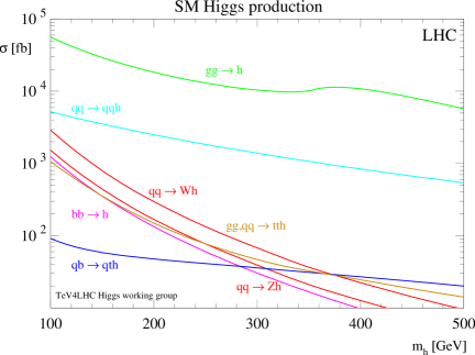
Figure 4: The various production cross sections for a SM-like Higgs boson at the LHC are shown as a function of $M_{H}^{\rm SM}$ (taken from Ref. [15], where also the relevant references can be found).

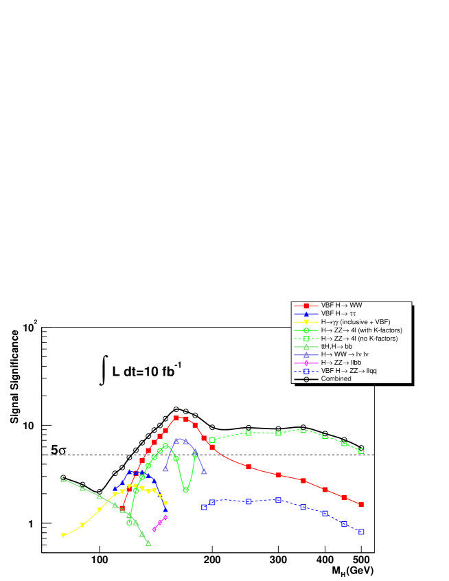
Figure 5: Significance of a Higgs signal, measured at ATLAS with $10\,\mbox{fb}^{-1}$ [16]. Similar results have been obtained for CMS [17].

2.4 Electroweak precision observables

Within the SM the electroweak precision observables (EWPO) have been used to constrain the last unknown parameter of the model, the Higgs-boson mass $M_{H}^{\rm SM}$. Originally the EWPO comprise over thousand measurements of “realistic observables” (with partially correlated uncertainties) such as cross sections, asymmetries, branching ratios etc. This huge set is reduced to 17 so-called “pseudo observables” by the LEP [18] and Tevatron [19] Electroweak working groups. The “pseudo observables” (again called EWPO in the following) comprise the $W$ boson mass $M_{W}$, the width of the $W$ boson, $\Gamma_{W}$, as well as various $Z$ pole observables: the effective weak mixing angle, $\sin^{2}\theta_{\mathrm{eff}}$, $Z$ decay widths to SM fermions, $\Gamma(Z\to f\bar{f})$, the invisible and total width, $\Gamma_{\rm inv}$ and $\Gamma_{Z}$, forward-backward and left-right asymmetries, $A_{\rm FB}^{f}$ and $A_{\rm LR}^{f}$, and the total hadronic cross section, $\sigma^{0}_{\rm had}$. The $Z$ pole results including their combination are final [20]. Experimental progress from the Tevatron comes for $M_{W}$ and $m_{t}$. (Also the error combination for $M_{W}$ and $\Gamma_{W}$ from the four LEP experiments has not been finalized yet due to not-yet-final analyses on the color-reconnection effects.)

The EWPO that give the strongest constraints on $M_{H}^{\rm SM}$ are $M_{W}$, $A_{\rm FB}^{b}$ and $A_{\rm LR}^{e}$. The value of $\sin^{2}\theta_{\mathrm{eff}}$ is extracted from a combination of various $A_{\rm FB}^{f}$ and $A_{\rm LR}^{f}$, where $A_{\rm FB}^{b}$ and $A_{\rm LR}^{e}$ give the dominant contribution.

The one-loop contributions to $M_{W}$ can be decomposed as follows [21],

$$M_{W}^{2}\left(1-\frac{M_{W}^{2}}{M_{Z}^{2}}\right) =\frac{\pi\alpha}{\sqrt{2}G_{F}}\left(1+\Delta r\right),$$ (61)

$$\Delta r_{1-{\rm loop}} =\Delta\alpha-\frac{c_{\mathrm{w}}^{2}}{s_{\mathrm{w}}^{2}}\Delta\rho+\Delta r_{\rm rem}(M_{H}^{\rm SM}).$$ (62)

The first term, $\Delta\alpha$ contains large logarithmic contributions as $\log(M_{Z}/m_{f})$ and amounts $\sim 6\%$. The second term contains the $\rho$ parameter [22], being $\Delta\rho\sim m_{t}^{2}$. This term amounts $\sim 3.3\%$. The quantity $\Delta\rho$,

$$\Delta\rho =\frac{\Sigma^{Z}(0)}{M_{Z}^{2}}-\frac{\Sigma^{W}(0)}{M_{W}^{2}},$$ (63)

parameterizes the leading universal corrections to the electroweak precision observables induced by the mass splitting between fields in an isospin doublet. $\Sigma^{Z,W}(0)$ denote the transverse parts of the unrenormalized $Z$ and $W$ boson self-energies at zero momentum transfer, respectively. The final term in Eq. (62) is $\Delta r_{\rm rem}\sim\log(M_{H}^{\rm SM}/M_{W})$, and with a size of $\sim 1\%$ correction yields the constraints on $M_{H}^{\rm SM}$. The fact that the leading correction involving $M_{H}^{\rm SM}$ is logarithmic also applies to the other EWPO. Starting from two-loop order, also terms $\sim(M_{H}^{\rm SM}/M_{W})^{2}$ appear. The SM prediction of $M_{W}$ as a function of $m_{t}$ for the range $M_{H}^{\rm SM}=114\,\,\mathrm{GeV}\ldots 1000\,\,\mathrm{GeV}$ is shown as the dark shaded (green) band in Figure 6 [18]. The upper edge with $M_{H}^{\rm SM}=114\,\,\mathrm{GeV}$ corresponds to the lower limit on $M_{H}^{\rm SM}$ obtained at LEP [23]. The prediction is compared with the direct experimental result [24, 25],

$$M_{W}^{\rm exp} =80.399\pm 0.023\,\,\mathrm{GeV}~{},$$ (64)

$$m_{t}^{\rm exp} =173.1\pm 1.3\,\,\mathrm{GeV}~{},$$ (65)

shown as the dotted (blue) ellipse and with the indirect results for $M_{W}$ and $m_{t}$ as obtained from EWPO (solid/red ellipse). The direct and indirect determination have significant overlap, representing a non-trivial success for the SM. However, it should be noted that the experimental value of $M_{W}$ is somewhat higher than the region allowed by the LEP Higgs bounds: $M_{H}^{\rm SM}\approx 60\,\,\mathrm{GeV}$ is preferred as a central value by the measurement of $M_{W}$ and $m_{t}$.

  

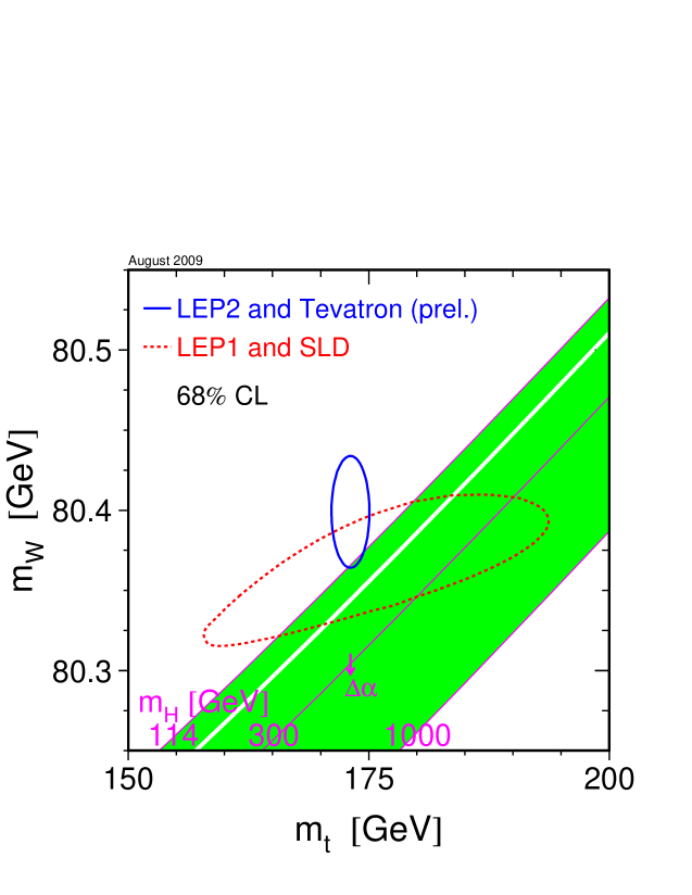
Figure 6: Prediction for $M_{W}$ in the SM as a function of $m_{t}$ for the range $M_{H}^{\rm SM}=114\,\,\mathrm{GeV}\ldots 1000\,\,\mathrm{GeV}$ [18]. The prediction is compared with the present experimental results for $M_{W}$ and $m_{t}$ as well as with the indirect constraints obtained from EWPO.

The effective weak mixing angle is evaluated from various asymmetries and other EWPO as shown in Figure 7 [26]. The average determination yields $\sin^{2}\theta_{\mathrm{eff}}=0.23153\pm 0.00016$ with a $\chi^{2}/{\rm d.o.f}$ of $11.8/5$, corresponding to a probability of $3.7\%$ [26]. The large $\chi^{2}$ is driven by the two single most precise measurements, $A_{\rm LR}^{e}$ by SLD and $A_{\rm FB}^{b}$ by LEP, where the earlier (latter) one prefers a value of $M_{H}^{\rm SM}\sim 32(437)\,\,\mathrm{GeV}$ [27]. The two measurements differ by more than $3\,\sigma$. The averaged value of $\sin^{2}\theta_{\mathrm{eff}}$, as shown in Figure 7, prefers $M_{H}^{\rm SM}\sim 110\,\,\mathrm{GeV}$ [27].

  

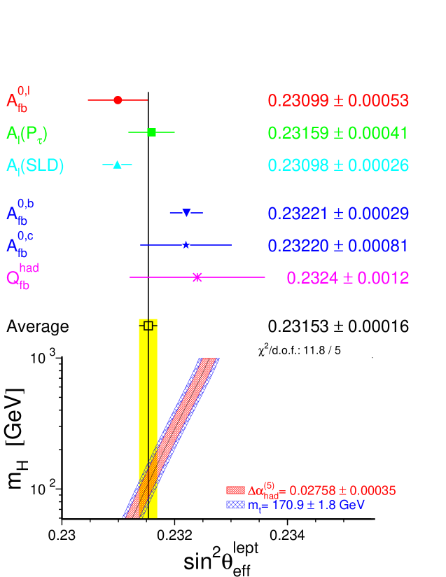
Figure 7: Prediction for $\sin^{2}\theta_{\mathrm{eff}}$ in the SM as a function of $M_{H}^{\rm SM}$ for $m_{t}=170.9\pm 1.8\,\,\mathrm{GeV}$ and $\Delta\alpha_{\rm had}^{5}=0.02758\pm 0.00035$ [26]. The prediction is compared with the present experimental results for $\sin^{2}\theta_{\mathrm{eff}}$ as averaged over several individual measurements.

The indirect $M_{H}^{\rm SM}$ determination for several individual EWPO is given in Figure 8. Shown are the central values of $M_{H}^{\rm SM}$ and the one $\sigma$ errors [18]. The dark shaded (green) vertical band indicates the combination of the various single measurements in the $1\,\sigma$ range. The vertical line shows the lower LEP bound for $M_{H}^{\rm SM}$ [23]. It can be seen that $M_{W}$, $A_{\rm LR}^{e}$ and $A_{\rm FB}^{b}$ give the most precise indirect $M_{H}^{\rm SM}$ determination, where only the latter one pulls the preferred $M_{H}^{\rm SM}$ value up, yielding a averaged value of [18]

$$M_{H}^{\rm SM}=87^{+35}_{-26}\,\,\mathrm{GeV}~{},$$ (66)

still compatible with the direct LEP bound of [23]

$$M_{H}^{\rm SM}\geq 114.4\,\,\mathrm{GeV}\mbox{~{}at~{}}95\%\mbox{~{}C.L.}$$ (67)

Thus, the measurement of $A_{\rm FB}^{b}$ prevents the SM from being incompatible with the direct bound and the indirect constraints on $M_{H}^{\rm SM}$.

  

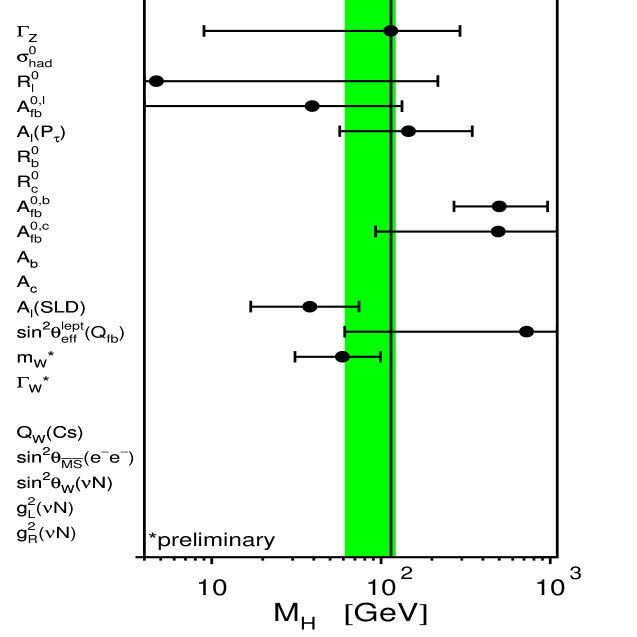
Figure 8: Indirect constrains on $M_{H}^{\rm SM}$ from various EWPO. Shown are the central values and the one $\sigma$ errors [18]. The dark shaded (green) vertical band indicates the combination of the various single measurements in the $1\,\sigma$ range. The vertical line shows the lower bound of $M_{H}^{\rm SM}\geq 114.4\,\,\mathrm{GeV}$ obtained at LEP [23].

In the left plot of Figure 9 [18] we show the result for the global fit to $M_{H}^{\rm SM}$ including all EWPO, but not including the direct search bounds from LEP and the Tevatron. $\Delta\chi^{2}$ is shown as a function of $M_{H}^{\rm SM}$, yielding Eq. (66) as best fit with an upper limit of $157\,\,\mathrm{GeV}$ at 95% C.L. The theory (intrinsic) uncertainty in the SM calculations (as evaluated with TOPAZ0 [28] and ZFITTER [29]) are represented by the thickness of the blue band. The width of the parabola itself, on the other hand, is determined by the experimental precision of the measurements of the EWPO and the input parameters. The result changes somewhat if the direct bounds on $M_{H}^{\rm SM}$ from LEP [23] and the Tevatron [30] are taken into account as shown in the right plot of Figure 9. The upper limit reduced to $M_{H}^{\rm SM}\mathrel{\raise 2.15277pt\hbox{$<$}\kern-7.44856pt\lower 4.0pt\hbox{{$\displaystyle\sim$}}}150\,\,\mathrm{GeV}$ at the 95% C.L. [31]. In this analysis an Tevatron exclusion of $160\,\,\mathrm{GeV}<M_{H}^{\rm SM}<170\,\,\mathrm{GeV}$ [30] was assumed. The most recent limit is slightly smaller, $163\,\,\mathrm{GeV}<M_{H}^{\rm SM}<166\,\,\mathrm{GeV}$ [32], however the picture is expected to vary only very little with this shift.

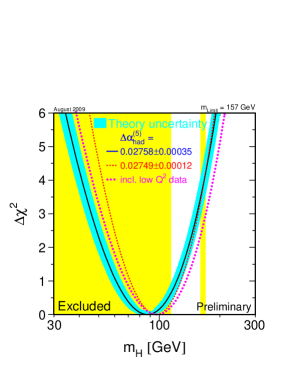
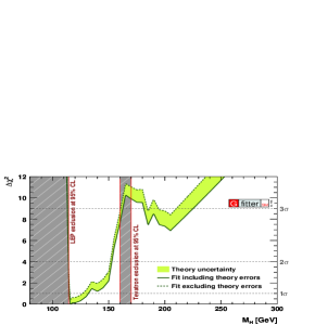
Figure 9: $\Delta\chi^{2}$ curve derived from all EWPO measured at LEP, SLD, CDF and D0, as a function of $M_{H}^{\rm SM}$, assuming the SM to be the correct theory of nature. Left: the direct bounds on $M_{H}^{\rm SM}$ are not included [18], right: the bounds from LEP [23] and the Tevatron [32] are included [31].

The current and anticipated future experimental uncertainties for $\sin^{2}\theta_{\mathrm{eff}}$, $M_{W}$ and $m_{t}$ are summarized in Tab. 1. Also shown is the relative precision of the indirect determination of $M_{H}^{\rm SM}$ [26]. Each column represents the combined results of all detectors and channels at a given collider, taking into account correlated systematic uncertainties, see Refs. [33, 34, 35, 36] for details. The indirect $M_{H}^{\rm SM}$ determination has to be compared with the (possible) direct measurement at the LHC [16, 17] and the ILC [37],

$$\delta M_{H}^{\rm SM}\mbox{}^{\rm,exp,LHC} \approx 200\,\,\mathrm{MeV},$$ (68)

$$\delta M_{H}^{\rm SM}\mbox{}^{\rm,exp,ILC} \approx 50\,\,\mathrm{MeV}.$$ (69)

	now	Tevatron	LHC	ILC	ILC with GigaZ
$\delta\sin^{2}\theta_{\mathrm{eff}}(\times 10^{5})$	16	—	14–20	—	1.3
$\delta M_{W}$ [MeV]	23	20	15	10	7
$\delta m_{t}$ [GeV]	1.3	1.0	1.0	0.2	0.1
$\delta M_{H}^{\rm SM}/M_{H}^{\rm SM}$ [%]	37		28		16

Table 1: Current and anticipated future experimental uncertainties for $\sin^{2}\theta_{\mathrm{eff}}$, $M_{W}$ and $m_{t}$. Also shown is the relative precision of the indirect determination of $M_{H}^{\rm SM}$ [26]. Each column represents the combined results of all detectors and channels at a given collider, taking into account correlated systematic uncertainties, see Refs. [33, 34, 35, 36] for details.

This comparison will shed light on the basic theoretical components for generating the masses of the fundamental particles. On the other hand, an observed inconsistency would be a clear indication for the existence of a new physics scale.

3 The Higgs in Supersymmetry

3.1 Why SUSY?

Theories based on Supersymmetry (SUSY) [5] are widely considered as the theoretically most appealing extension of the SM. They are consistent with the approximate unification of the gauge coupling constants at the GUT scale and provide a way to cancel the quadratic divergences in the Higgs sector hence stabilizing the huge hierarchy between the GUT and the Fermi scales. Furthermore, in SUSY theories the breaking of the electroweak symmetry is naturally induced at the Fermi scale, and the lightest supersymmetric particle can be neutral, weakly interacting and absolutely stable, providing therefore a natural solution for the dark matter problem.

The Minimal Supersymmetric Standard Model (MSSM) constitutes, hence its name, the minimal supersymmetric extension of the SM. The number of SUSY generators is $N=1$, the smallest possible value. In order to keep anomaly cancellation, contrary to the SM a second Higgs doublet is needed [38]. All SM multiplets, including the two Higgs doublets, are extended to supersymmetric multiplets, resulting in scalar partners for quarks and leptons (“squarks” and “sleptons”) and fermionic partners for the SM gauge boson and the Higgs bosons (“gauginos” and “gluinos”). So far, the direct search for SUSY particles has not been successful. One can only set lower bounds of ${\cal O}(100\,\,\mathrm{GeV})$ on their masses [39].

3.2 The MSSM Higgs sector

An excellent review on this subject is given in Ref. [40].

3.2.1 The Higgs boson sector at tree-level

Contrary to the Standard Model (SM), in the MSSM two Higgs doublets are required. The Higgs potential [41]

$$V =m_{1}^{2}|{\cal H}_{1}|^{2}+m_{2}^{2}|{\cal H}_{2}|^{2}-m_{12}^{2}(\epsilon_{ab}{\cal H}_{1}^{a}{\cal H}_{2}^{b}+\mbox{h.c.})$$

$$+\frac{1}{8}(g^{2}+g^{\prime 2})\left[|{\cal H}_{1}|^{2}-|{\cal H}_{2}|^{2}\right]^{2}+\frac{1}{2}g^{2}|{\cal H}_{1}^{{\dagger}}{\cal H}_{2}|^{2}~{},$$ (70)

contains $m_{1},m_{2},m_{12}$ as soft SUSY breaking parameters; $g,g^{\prime}$ are the $SU(2)$ and $U(1)$ gauge couplings, and $\epsilon_{12}=-1$.

The doublet fields $H_{1}$ and $H_{2}$ are decomposed in the following way:

$${\cal H}_{1} =\left(\begin{array}[]{c}{\cal H}_{1}^{0}\\[2.15277pt] {\cal H}_{1}^{-}\end{array}\right)\;=\;\left(\begin{array}[]{c}v_{1}+\frac{1}{\sqrt{2}}(\phi_{1}^{0}-i\chi_{1}^{0})\\[2.15277pt] -\phi_{1}^{-}\end{array}\right)~{},$$ (75)

$${\cal H}_{2} =\left(\begin{array}[]{c}{\cal H}_{2}^{+}\\[2.15277pt] {\cal H}_{2}^{0}\end{array}\right)\;=\;\left(\begin{array}[]{c}\phi_{2}^{+}\\[2.15277pt] v_{2}+\frac{1}{\sqrt{2}}(\phi_{2}^{0}+i\chi_{2}^{0})\end{array}\right)~{}.$$ (80)

${\cal H}_{1}$ gives mass to the down-type fermions, while ${\cal H}_{2}$ gives masses to the up-type fermions. The potential (70) can be described with the help of two independent parameters (besides $g$ and $g^{\prime}$): $\tan\beta=v_{2}/v_{1}$ and $M_{A}^{2}=-m_{12}^{2}(\tan\beta+\cot\beta)$, where $M_{A}$ is the mass of the ${\cal CP}$-odd Higgs boson $A$.

Which values can be expected for $\tan\beta$? One natural choice would be $\tan\beta\approx 1$, i.e. both vevs are about the same. On the other hand, one can argue that $v_{2}$ is responsible for the top quark mass, while $v_{1}$ gives rise to the bottom quark mass. Assuming that their mass differences comes largely from the vevs, while their Yukawa couplings could be about the same. The natural value for $\tan\beta$ would then be $\tan\beta\approx m_{t}/m_{b}$. Consequently, one can expect

$$1\mathrel{\raise 2.15277pt\hbox{$<$}\kern-7.44856pt\lower 4.0pt\hbox{{$\displaystyle\sim$}}}\tan\beta\mathrel{\raise 2.15277pt\hbox{$<$}\kern-7.44856pt\lower 4.0pt\hbox{{$\displaystyle\sim$}}}50~{}.$$ (81)

The diagonalization of the bilinear part of the Higgs potential, i.e. of the Higgs mass matrices, is performed via the orthogonal transformations

$$\left(\begin{array}[]{c}H^{0}\\[2.15277pt] h^{0}\end{array}\right) =\left(\begin{array}[]{cc}\cos\alpha&\sin\alpha\\[2.15277pt] -\sin\alpha&\cos\alpha\end{array}\right)\left(\begin{array}[]{c}\phi_{1}^{0}\\[2.15277pt] \phi_{2}^{0}~{},\end{array}\right)$$ (88)

$$\left(\begin{array}[]{c}G^{0}\\[2.15277pt] A^{0}\end{array}\right) =\left(\begin{array}[]{cc}\cos\beta&\sin\beta\\[2.15277pt] -\sin\beta&\cos\beta\end{array}\right)\left(\begin{array}[]{c}\chi_{1}^{0}\\[2.15277pt] \chi_{2}^{0}\end{array}\right)~{},$$ (95)

$$\left(\begin{array}[]{c}G^{\pm}\\[2.15277pt] H^{\pm}\end{array}\right) =\left(\begin{array}[]{cc}\cos\beta&\sin\beta\\[2.15277pt] -\sin\beta&\cos\beta\end{array}\right)\left(\begin{array}[]{c}\phi_{1}^{\pm}\\[2.15277pt] \phi_{2}^{\pm}\end{array}\right)~{}.$$ (102)

The mixing angle $\alpha$ is determined through

$$\alpha={\rm arctan}\left[\frac{-(M_{A}^{2}+M_{Z}^{2})\sin\beta\cos\beta}{M_{Z}^{2}\cos^{2}\beta+M_{A}^{2}\sin^{2}\beta-m^{2}_{h,{\rm tree}}}\right]~{},~{}~{}-\frac{\pi}{2}<\alpha<0$$ (103)

with $m_{h,{\rm tree}}$ defined below in Eq. (114).
One gets the following Higgs spectrum:

$$\mbox{2 neutral bosons},\,{\cal CP}=+1 :h,H$$

$$\mbox{1 neutral boson},\,{\cal CP}=-1 :A$$

2 charged bosons $$:H^{+},H^{-}$$

3 unphysical Goldstone bosons $$:G,G^{+},G^{-}.$$ (104)

At tree level the mass matrix of the neutral ${\cal CP}$-even Higgs bosons is given in the $\phi_{1}$-$\phi_{2}$-basis in terms of $M_{Z}$, $M_{A}$, and $\tan\beta$ by

$$M_{\rm Higgs}^{2,{\rm tree}} =\left(\begin{array}[]{cc}m_{\phi_{1}}^{2}&m_{\phi_{1}\phi_{2}}^{2}\\ m_{\phi_{1}\phi_{2}}^{2}&m_{\phi_{2}}^{2}\end{array}\right)$$ (107)

$$=\left(\begin{array}[]{cc}M_{A}^{2}\sin^{2}\beta+M_{Z}^{2}\cos^{2}\beta&-(M_{A}^{2}+M_{Z}^{2})\sin\beta\cos\beta\\ -(M_{A}^{2}+M_{Z}^{2})\sin\beta\cos\beta&M_{A}^{2}\cos^{2}\beta+M_{Z}^{2}\sin^{2}\beta\end{array}\right),$$ (110)

which by diagonalization according to Eq. (88) yields the tree-level Higgs boson masses

$$M_{\rm Higgs}^{2,{\rm tree}}\stackrel{{\scriptstyle\alpha}}{{\longrightarrow}}\left(\begin{array}[]{cc}m_{H,{\rm tree}}^{2}&0\\ 0&m_{h,{\rm tree}}^{2}\end{array}\right)$$ (113)

with

$$m_{H,h,{\rm tree}}^{2} =\frac{1}{2}\left[M_{A}^{2}+M_{Z}^{2}\pm\sqrt{(M_{A}^{2}+M_{Z}^{2})^{2}-4M_{Z}^{2}M_{A}^{2}\cos^{2}2\beta}\right]~{}.$$ (114)

From this formula the famous tree-level bound

$$m_{h,{\rm tree}}\leq\mbox{min}\{M_{A},M_{Z}\}\cdot|\cos 2\beta|\leq M_{Z}$$ (115)

can be obtained. The charged Higgs boson mass is given by

$$m_{H^{\pm}}^{2}=M_{A}^{2}+M_{W}^{2}~{}.$$ (116)

The masses of the gauge bosons are given in analogy to the SM:

$$M_{W}^{2}=\frac{1}{2}g^{2}(v_{1}^{2}+v_{2}^{2});\qquad M_{Z}^{2}=\frac{1}{2}(g^{2}+g^{\prime 2})(v_{1}^{2}+v_{2}^{2});\qquad M_{\gamma}=0.$$ (117)

The couplings of the Higgs bosons are modified from the corresponding SM couplings already at the tree-level. Some examples are

$$g_{hVV} =\sin(\beta-\alpha)\;g_{HVV}^{\rm SM},\quad V=W^{\pm},Z~{},$$ (118)

$$g_{HVV} =\cos(\beta-\alpha)\;g_{HVV}^{\rm SM}~{},$$ (119)

$$g_{hb\bar{b}},g_{h\tau^{+}\tau^{-}} =-\frac{\sin\alpha}{\cos\beta}\;g_{Hb\bar{b},H\tau^{+}\tau^{-}}^{\rm SM}~{},$$ (120)

$$g_{ht\bar{t}} =\frac{\cos\alpha}{\sin\beta}\;g_{Ht\bar{t}}^{\rm SM}~{},$$ (121)

$$g_{Ab\bar{b}},g_{A\tau^{+}\tau^{-}} =\gamma_{5}\tan\beta\;g_{Hb\bar{b},H\tau^{+}\tau^{-}}^{\rm SM}~{}.$$ (122)

The following can be observed: the couplings of the ${\cal CP}$-even Higgs boson to SM gauge bosons is always suppressed with respect to the SM coupling. However, if $g_{hVV}^{2}$ is close to zero, $g_{HVV}^{2}$ is close to $(g_{HVV}^{\rm SM})^{2}$ and vice versa, i.e. it is not possible to decouple both of them from the SM gauge bosons. The coupling of the $h$ to down-type fermions can be suppressed or enhanced with respect to the SM value, depending on the size of $\sin\alpha/\cos\beta$. Especially for not too large values of $M_{A}$ and large $\tan\beta$ one finds $|\sin\alpha/\cos\beta|\gg 1$, leading to a strong enhancement of this coupling. The same holds, in principle, for the coupling of the $h$ to up-type fermions. However, for large parts of the MSSM parameter space the additional factor is found to be $|\cos\alpha/\sin\beta|<1$. For the ${\cal CP}$-odd Higgs boson an additional factor $\tan\beta$ is found. According to Eq. (81) this can lead to a strongly enhanced coupling of the $A$ boson to bottom quarks or $\tau$ leptons, resulting in new search strategies at the Tevatron and the LHC for the ${\cal CP}$-odd Higgs boson, see Sect. 3.3.

For $M_{A}\mathrel{\raise 2.15277pt\hbox{$>$}\kern-7.44856pt\lower 4.0pt\hbox{{$\displaystyle\sim$}}}150\,\,\mathrm{GeV}$ the “decoupling limit” is reached. The couplings of the light Higgs boson become SM-like, i.e. the additional factors approach 1. The couplings of the heavy neutral Higgs bosons become similar, $g_{Axx}\approx g_{Hxx}$, and the masses of the heavy neutral and charged Higgs bosons fulfill $M_{A}\approx M_{H}\approx M_{H^{\pm}}$. As a consequence, search strategies for the $A$ boson can also be applied to the $H$ boson, and both are hard to disentangle at hadron colliders.

3.2.2 The scalar quark sector

Since the most relevant squarks for the MSSM Higgs boson sector are the $\tilde{t}$ and $\tilde{b}$ particles, here we explicitly list their mass matrices in the basis of the gauge eigenstates $\tilde{t}_{L},\tilde{t}_{R}$ and $\tilde{b}_{L},\tilde{b}_{R}$:

$${\cal M}^{2}_{\tilde{t}} =\left(\begin{array}[]{cc}M_{\tilde{t}_{L}}^{2}+m_{t}^{2}+\cos 2\beta(\frac{1}{2}-\frac{2}{3}s_{\mathrm{w}}^{2})M_{Z}^{2}&m_{t}X_{t}\\ m_{t}X_{t}&M_{\tilde{t}_{R}}^{2}+m_{t}^{2}+\frac{2}{3}\cos 2\beta s_{\mathrm{w}}^{2}M_{Z}^{2}\end{array}\right),$$ (125)

$${\cal M}^{2}_{\tilde{b}} =\left(\begin{array}[]{cc}M_{\tilde{b}_{L}}^{2}+m_{b}^{2}+\cos 2\beta(-\frac{1}{2}+\frac{1}{3}s_{\mathrm{w}}^{2})M_{Z}^{2}&m_{b}X_{b}\\ m_{b}X_{b}&M_{\tilde{b}_{R}}^{2}+m_{b}^{2}-\frac{1}{3}\cos 2\beta s_{\mathrm{w}}^{2}M_{Z}^{2}\end{array}\right).$$ (128)

$M_{\tilde{t}_{L}}$, $M_{\tilde{t}_{R}}$, $M_{\tilde{b}_{L}}$ and $M_{\tilde{b}_{R}}$ are the (diagonal) soft SUSY-breaking parameters. We furthermore have

$$m_{t}X_{t}=m_{t}(A_{t}-\mu\cot\beta),\quad m_{b}\,X_{b}=m_{b}\,(A_{b}-\mu\tan\beta).$$ (129)

The soft SUSY-breaking parameters $A_{t}$ and $A_{b}$ denote the trilinear Higgs–stop and Higgs–sbottom coupling, and $\mu$ is the Higgs mixing parameter. $SU(2)$ gauge invariance requires the relation

$$M_{\tilde{t}_{L}}=M_{\tilde{b}_{L}}.$$ (130)

Diagonalizing ${\cal M}^{2}_{\tilde{t}}$ and ${\cal M}^{2}_{\tilde{b}}$ with the mixing angles $\theta_{\tilde{t}}$ and $\theta_{\tilde{b}}$, respectively, yields the physical $\tilde{t}$ and $\tilde{b}$ masses: $m_{\tilde{t}_{1}}$, $m_{\tilde{t}_{2}}$, $m_{\tilde{b}_{1}}$ and $m_{\tilde{b}_{2}}$.

3.2.3 Higher-order corrections to Higgs boson masses

A review about this subject can be found in Ref. [42]. In the Feynman diagrammatic (FD) approach the higher-order corrected ${\cal CP}$-even Higgs boson masses in the rMSSM are derived by finding the poles of the $(h,H)$-propagator matrix. The inverse of this matrix is given by

$$\left(\Delta_{\rm Higgs}\right)^{-1}=-i\left(\begin{array}[]{cc}p^{2}-m_{H,{\rm tree}}^{2}+\hat{\Sigma}_{HH}(p^{2})&\hat{\Sigma}_{hH}(p^{2})\\ \hat{\Sigma}_{hH}(p^{2})&p^{2}-m_{h,{\rm tree}}^{2}+\hat{\Sigma}_{hh}(p^{2})\end{array}\right)~{}.$$ (131)

Determining the poles of the matrix $\Delta_{\rm Higgs}$ in Eq. (131) is equivalent to solving the equation

$$\left[p^{2}-m_{h,{\rm tree}}^{2}+\hat{\Sigma}_{hh}(p^{2})\right]\left[p^{2}-m_{H,{\rm tree}}^{2}+\hat{\Sigma}_{HH}(p^{2})\right]-\left[\hat{\Sigma}_{hH}(p^{2})\right]^{2}=0\,.$$ (132)

The very leading one-loop correction to $M_{h}^{2}$ is given by

$$\Delta M_{h}^{2} =G_{F}m_{t}^{4}\log\left(\frac{m_{\tilde{t}_{1}}m_{\tilde{t}_{2}}}{m_{t}^{2}}\right)~{},$$ (133)

where $G_{F}$ denotes the Fermi constant. The Eq. (133) shows two important aspects: First, the leading loop corrections go with $m_{t}^{4}$, which is a “very large number”. Consequently, the loop corrections can strongly affect $M_{h}$ and push the mass beyond the reach of LEP [23, 43]. Second, the scalar fermion masses (in this case the scalar top masses) appear in the log entering the loop corrections (acting as a “cut-off” where the new physics enter). In this way the light Higgs boson mass depends on all other sectors via loop corrections. This dependence is particularly pronounced for the scalar top sector due to the large mass of the top quark.

The status of the available results for the self-energy contributions to Eq. (131) can be summarized as follows. For the one-loop part, the complete result within the MSSM is known [44, 45, 46, 47]. The by far dominant one-loop contribution is the ${\cal O}(\alpha_{t})$ term due to top and stop loops, see also Eq. (133), ($\alpha_{t}\equiv h_{t}^{2}/(4\pi)$, $h_{t}$ being the superpotential top coupling). Concerning the two-loop effects, their computation is quite advanced and has now reached a stage such that all the presumably dominant contributions are known. They include the strong corrections, usually indicated as ${\cal O}(\alpha_{t}\alpha_{s})$, and Yukawa corrections, ${\cal O}(\alpha_{t}^{2})$, to the dominant one-loop ${\cal O}(\alpha_{t})$ term, as well as the strong corrections to the bottom/sbottom one-loop ${\cal O}(\alpha_{b})$ term ($\alpha_{b}\equiv h_{b}^{2}/(4\pi)$), i.e. the ${\cal O}(\alpha_{b}\alpha_{s})$ contribution. The latter can be relevant for large values of $\tan\beta$. Presently, the ${\cal O}(\alpha_{t}\alpha_{s})$ [48, 49, 50, 51, 52], ${\cal O}(\alpha_{t}^{2})$ [48, 53, 54] and the ${\cal O}(\alpha_{b}\alpha_{s})$ [55, 56] contributions to the self-energies are known for vanishing external momenta. In the (s)bottom corrections the all-order resummation of the $\tan\beta$-enhanced terms, ${\cal O}(\alpha_{b}(\alpha_{s}\tan\beta)^{n})$, is also performed [57, 58]. The ${\cal O}(\alpha_{t}\alpha_{b})$ and ${\cal O}(\alpha_{b}^{2})$ corrections were presented in Ref. [59]. A “nearly full” two-loop effective potential calculation (including even the momentum dependence for the leading pieces and the leading three-loop corrections) has been published [60]. Most recently another leading three-loop calculation, valid for certain SUSY mass combinations, became available [61]. Taking the available loop corrections into account, the upper limit of $M_{h}$ is shifted to [62],

$$M_{h}\leq 135\,\,\mathrm{GeV}~{}$$ (134)

(as obtained with the code FeynHiggs [63, 50, 62, 64]). This limit takes into account the experimental uncertainty for the top quark mass, see Eq. (65), as well as the intrinsic uncertainties from unknown higher-order corrections [62, 71].

The charged Higgs boson mass is obtained by solving the equation

$$p^{2}-m_{H^{\pm}}^{2}-\hat{\Sigma}_{H^{-}H^{+}}(p^{2})=0~{}.$$ (135)

The charged Higgs boson self-energy is known at the one-loop level [65, 66].

3.3 MSSM Higgs boson searches at the LHC

The “decoupling limit” has been discussed for the tree-level couplings and masses of the MSSM Higgs bosons in Sect. 3.2.1. This limit also persists taking into account radiative corrections. The corresponding Higgs boson masses are shown in Figure 10 for $\tan\beta=5$ in the $m_{h}^{\rm max}$ benchmark scenario [67] obtained with FeynHiggs. For $M_{A}\mathrel{\raise 2.15277pt\hbox{$>$}\kern-7.44856pt\lower 4.0pt\hbox{{$\displaystyle\sim$}}}150\,\,\mathrm{GeV}$ the lightest Higgs boson mass approaches its upper limit (depending on the SUSY parameters), and the heavy Higgs boson masses are nearly degenerate. Furthermore, also the light Higgs boson couplings including loop corrections approach their SM-value for. Consequently, for $M_{A}\mathrel{\raise 2.15277pt\hbox{$>$}\kern-7.44856pt\lower 4.0pt\hbox{{$\displaystyle\sim$}}}150\,\,\mathrm{GeV}$ the experimental searches for the lightest MSSM Higgs boson, see Sect. 2.3, can be performed very similarly to the SM Higgs boson searches (with $M_{H}^{\rm SM}=M_{h}$).

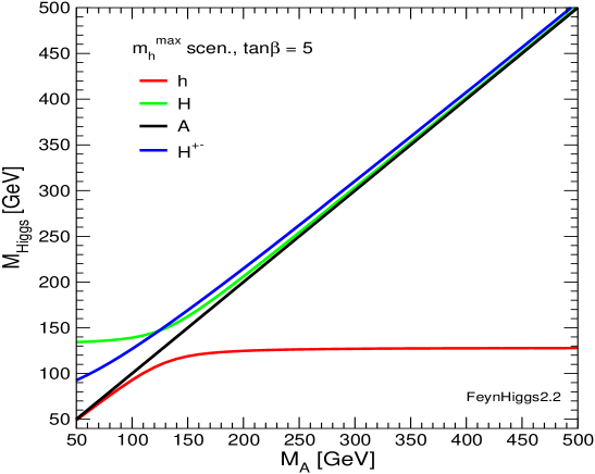
Figure 10: The MSSM Higgs boson masses including higher-order corrections are shown as a function of $M_{A}$ for $\tan\beta=5$ in the $m_{h}^{\rm max}$ benchmark scenario [67] (obtained with FeynHiggs [63, 50, 62, 64]).

The various productions cross sections at the LHC are shown in Figure 11 (for $\sqrt{s}=14\,\,\mathrm{TeV}$). For low masses the light Higgs cross sections are visible, and for $M_{H}\mathrel{\raise 2.15277pt\hbox{$>$}\kern-7.44856pt\lower 4.0pt\hbox{{$\displaystyle\sim$}}}130\,\,\mathrm{GeV}$ the heavy ${\cal CP}$-even Higgs cross section is displayed, while the cross sections for the ${\cal CP}$-odd $A$ boson are given for the whole mass range. As discussed in Sect. 3.2.1 the $g_{Abb}$ coupling is enhanced by $\tan\beta$ with respect to the corresponding SM value. Consequently, the $b\bar{b}A$ cross section is the largest or second largest cross section for all $M_{A}$, despite the relatively small value of $\tan\beta=5$. For larger $\tan\beta$, see Eq. (81), this cross section can become even more dominant. Furthermore, the coupling of the heavy ${\cal CP}$-even Higgs boson becomes very similar to the one of the $A$ boson, and the two production cross sections, $b\bar{b}A$ and $b\bar{b}H$ are indistinguishable in the plot for $M_{A}>200\,\,\mathrm{GeV}$.

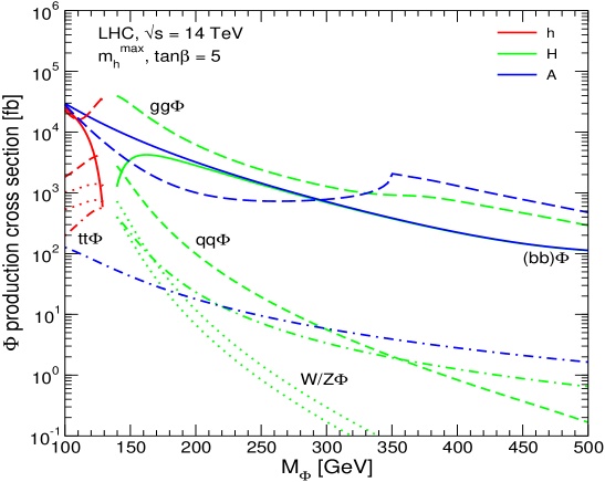
Figure 11: Overview about the various neutral Higgs boson production cross sections at the LHC shown as a function of $M_{A}$ for $\tan\beta=5$ in the $m_{h}^{\rm max}$ scenario (taken from Ref. [15], where the original references can be found).

Following the above discussion, the main search channel for heavy Higgs bosons at the LHC for $M_{A}\mathrel{\raise 2.15277pt\hbox{$>$}\kern-7.44856pt\lower 4.0pt\hbox{{$\displaystyle\sim$}}}200\,\,\mathrm{GeV}$ is the production in association with bottom quarks and the subsequent decay to tau leptons, $b\bar{b}\to b\bar{b}\;H/A\to b\bar{b}\;\tau^{+}\tau^{-}$. For heavy supersymmetric particles, with masses far above the Higgs boson mass scale, one has for the production and decay of the $A$ boson [68]

$$\sigma(b\bar{b}A)\times{\rm BR}(A\to b\bar{b})\simeq\sigma(b\bar{b}H)_{\rm SM}\;\frac{\tan^{2}\beta}{\left(1+\Delta_{b}\right)^{2}}\times\frac{9}{\left(1+\Delta_{b}\right)^{2}+9}~{},$$ (136)

$$\sigma(gg,b\bar{b}\to A)\times{\rm BR}(A\to\tau^{+}\tau^{-})\simeq\sigma(gg,b\bar{b}\to H)_{\rm SM}\;\frac{\tan^{2}\beta}{\left(1+\Delta_{b}\right)^{2}+9}~{},$$ (137)

where $\sigma(b\bar{b}H)_{\rm SM}$ and $\sigma(gg,b\bar{b}\to H)_{\rm SM}$ denote the values of the corresponding SM Higgs boson production cross sections for $M_{H}^{\rm SM}=M_{A}$. $\Delta_{b}$ is given by [57]

$$\Delta_{b}=\frac{2\alpha_{s}}{3\,\pi}\,m_{\tilde{g}}\,\mu\,\tan\beta\,\times\,I(m_{\tilde{b}_{1}},m_{\tilde{b}_{2}},m_{\tilde{g}})+\frac{\alpha_{t}}{4\,\pi}\,A_{t}\,\mu\,\tan\beta\,\times\,I(m_{\tilde{t}_{1}},m_{\tilde{t}_{2}},|\mu|)~{},$$ (138)

where the function $I$ arises from the one-loop vertex diagrams and scales as $I(a,b,c)\sim 1/\mbox{max}(a^{2},b^{2},c^{2})$. Here $m_{\tilde{g}}$ is the gluino mass, and $\mu$ is the Higgs mixing parameter. As a consequence, the $b\bar{b}$ production rate depends sensitively on $\Delta_{b}\propto\mu\,\tan\beta$ because of the factor $1/(1+\Delta_{b})^{2}$, while this leading dependence on $\Delta_{b}$ cancels out in the $\tau^{+}\tau^{-}$ production rate. The formulas above apply, within a good approximation, also to the heavy ${\cal CP}$-even Higgs boson in the large $\tan\beta$ regime. Therefore, the production and decay rates of $H$ are governed by similar formulas as the ones given above, leading to an approximate enhancement by a factor 2 of the production rates with respect to the ones that would be obtained in the case of the single production of the ${\cal CP}$-odd Higgs boson as given in Eqs. (136), (137).

Of particular interest is the “LHC wedge” region, i.e. the region in which only the light ${\cal CP}$-even MSSM Higgs boson, but non of the heavy MSSM Higgs bosons can be detected at the LHC at the 5$\,\sigma$ level. It appears for $M_{A}\mathrel{\raise 2.15277pt\hbox{$>$}\kern-7.44856pt\lower 4.0pt\hbox{{$\displaystyle\sim$}}}200\,\,\mathrm{GeV}$ at intermediate $\tan\beta$ and widens to larger $\tan\beta$ values for larger $M_{A}$. Consequently, in the “LHC wedge” only a SM-like light Higgs boson can be discovered at the LHC. This region is bounded from above by the $5\,\sigma$ discovery contours for the heavy neutral MSSM Higgs bosons as described above. These discovery contours depend sensitively on the Higgs mass parameter $\mu$. The dependence on $\mu$ enters in two different ways, on the one hand via higher-order corrections through $\Delta_{b}\propto\mu\,\tan\beta$, and on the other hand via the kinematics of Higgs decays into charginos and neutralinos, where $\mu$ enters in their respective mass matrices [5].

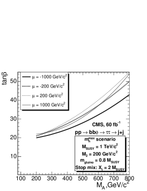
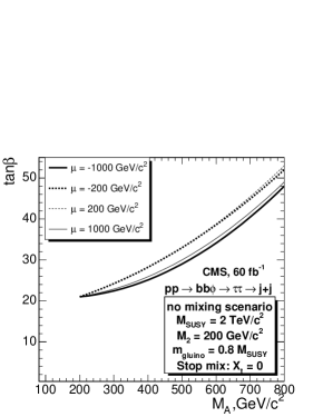
Figure 12: The $5\,\sigma$ discovery regions (i.e. the upper bound of the “LHC wedge” region) for the heavy neutral Higgs bosons in the channel $b\bar{b}\to b\bar{b}\;H/A,H/A\to\tau^{+}\tau^{-}\to\mbox{jets}$ (taken from Ref. [69]).

In Figure 12 we show the $5\,\sigma$ discovery regions for the heavy neutral MSSM Higgs bosons in the channel $b\bar{b}\to b\bar{b}\;H/A,H/A\to\tau^{+}\tau^{-}\to\mbox{jets}$ [69]. As explained above, these discovery contours correspond to the upper bound of the “LHC wedge”. A strong variation with the sign and the size of $\mu$ can be observed and should be taken into account in experimental and phenomenological analyses. The same higher-order corrections are relevant once a possible heavy Higgs boson signal at the LHC will be interpreted in terms of the underlying parameter space. From Eq. (138) it follows that an observed production cross section can be correctly connected to $\mu$ and $\tan\beta$ only if the scalar top and bottom masses, the gluino mass and the trilinear Higgs-stop coupling are measured and taken properly into account.

3.4 Electroweak precision observables

Also within SUSY one can attempt to fit the unknown parameters to the existing experimental data, in a similar fashion as it was discussed in Sect. 2.4. However, fits within the MSSM differs from the SM fit in various ways. First, the number of free parameters is substantially larger in the MSSM, even restricting to GUT based models as discussed below. On the other hand, more observables can be taken into account, providing extra constraints on the fit. Within the MSSM the additional observables included are the anomalous magnetic moment of the muon $(g-2)_{\mu}$, $B$-physics observables such as ${\rm BR}(b\to s\gamma)$ or ${\rm BR}(B_{s}\to\mu\mu)$, and the relic density of cold dark matter (CDM), which can be provided by the lightest SUSY particle, the neutralino. These additional constraints would either have a minor impact on the best-fit regions or cannot be accommodated in the SM. Finally, as discussed in the previous subsections, whereas the light Higgs boson mass is a free parameter in the SM, it is a function of the other parameters in the MSSM. In this way, for example, the masses of the scalar tops and bottoms enter not only directly into the prediction of the various observables, but also indirectly via their impact on $M_{h}$.

Within the MSSM the dominant SUSY correction to electroweak precision observables arises from the scalar top and bottom contribution to the $\rho$ parameter, see Eq. (63). The leading diagrams are shown in Figure 13.

Figure 13: Feynman diagrams for the contribution of scalar quark loops to the gauge boson self-energies at one-loop order, $V=W,Z$, $\tilde{q}=\tilde{t},\tilde{b}$.

Generically one finds $\Delta\rho^{\mathrm{SUSY}}>0$, leading, for instance, to an upward shift in the prediction of $M_{W}$ with respect to the SM prediction. The experimental result and the theory prediction of the SM and the MSSM for $M_{W}$ are compared in Figure 14 (updated from Ref. [70]). The predictions within the two models give rise to two bands in the $m_{t}$–$M_{W}$ plane with only a relatively small overlap sliver (indicated by a dark-shaded (blue) area in Figure 14). The allowed parameter region in the SM (the medium-shaded (red) and dark-shaded (blue) bands, corresponding to the SM prediction in Figure 6) arises from varying the only free parameter of the model, the mass of the SM Higgs boson, from $M_{H}^{\rm SM}=114\,\,\mathrm{GeV}$, the LEP exclusion bound [23] (upper edge of the dark-shaded (blue) area), to $400\,\,\mathrm{GeV}$ (lower edge of the medium-shaded (red) area). The light shaded (green) and the dark-shaded (blue) areas indicate allowed regions for the unconstrained MSSM, obtained from scattering the relevant parameters independently [70]. The decoupling limit with SUSY masses of ${\cal O}(2\,\,\mathrm{TeV})$ yields the lower edge of the dark-shaded (blue) area. Thus, the overlap region between the predictions of the two models corresponds in the SM to the region where the Higgs boson is light, i.e. in the MSSM allowed region ($M_{h}\mathrel{\raise 2.15277pt\hbox{$<$}\kern-7.44856pt\lower 4.0pt\hbox{{$\displaystyle\sim$}}}135\,\,\mathrm{GeV}$, see Eq. (134)). In the MSSM it corresponds to the case where all superpartners are heavy, i.e. the decoupling region of the MSSM. The current 68 and 95% C.L. experimental results for $m_{t}$, Eq. (65), and $M_{W}$, Eq. (64), are also indicated in the plot. As can be seen from Figure 14, the current experimental 68% C.L. region for $m_{t}$ and $M_{W}$ exhibits a slight preference of the MSSM over the SM. This example indicates that the experimental measurement of $M_{W}$ in combination with $m_{t}$ prefers, within the MSSM, not too heavy SUSY mass scales.

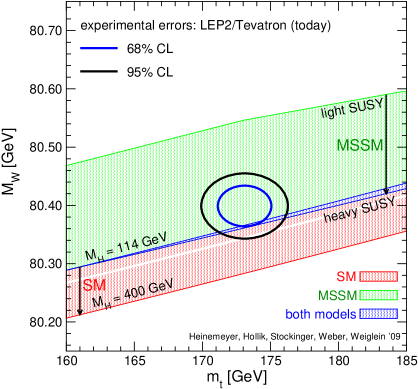
\begin{picture}(0.0,0.0) \put(0.0,0.0){} \put(0.0,0.0){} \end{picture}

Figure 14: Prediction for $M_{W}$ in the MSSM and the SM (see text) as a function of $m_{t}$ in comparison with the present experimental results for $M_{W}$ and $m_{t}$ (updated from Ref. [70], see Ref. [71] for details).

As mentioned above, in order to restrict the number of free parameters in the MSSM one can resort to GUT based models. Most fits have been performed in the Constrained MSSM (CMSSM), in which the input scalar masses $m_{0}$, gaugino masses $m_{1/2}$ and soft trilinear parameters $A_{0}$ are each universal at the GUT scale, $M_{\rm GUT}\approx 2\times 10^{16}\,\,\mathrm{GeV}$, and in the Non-universal Higgs mass model (NUHM1), in which a common SUSY-breaking contribution to the Higgs masses is allowed to be non-universal.

Here we follow the results obtained in Refs. [72, 73, 74], where an overview about different fitting techniques and extensive list of references can be found in Ref. [74]. The computer code used for the fits shown below is the MasterCode [72, 73, 74, 75], which includes the following theoretical codes. For the RGE running of the soft SUSY-breaking parameters, it uses SoftSUSY [76], which is combined consistently with the codes used for the various low-energy observables: FeynHiggs [63, 50, 62, 64] is used for the evaluation of the Higgs masses and $a_{\mu}^{\rm SUSY}$ (see also [77, 78, 79, 80]), for the other electroweak precision data we have included a code based on [70, 81], SuFla [82, 83] and SuperIso [84, 85] are used for flavor-related observables, and for dark-matter-related observables MicrOMEGAs [86] and DarkSUSY [87] are used. In the combination of the various codes, MasterCode makes extensive use of the SUSY Les Houches Accord [88, 89].

The global $\chi^{2}$ likelihood function, which combines all theoretical predictions with experimental constraints, is now given as

$$\chi^{2} =\sum^{N}_{i}\frac{(C_{i}-P_{i})^{2}}{\sigma(C_{i})^{2}+\sigma(P_{i})^{2}}+\sum^{M}_{i}\frac{(f^{\rm obs}_{{\rm SM}_{i}}-f^{\rm fit}_{{\rm SM}_{i}})^{2}}{\sigma(f_{{\rm SM}_{i}})^{2}}$$

$$+\chi^{2}({\rm BR}(B_{s}\to\mu\mu))+\chi^{2}(\mbox{SUSY search limits})$$ (139)

Here $N$ is the number of observables studied, $C_{i}$ represents an experimentally measured value (constraint) and each $P_{i}$ defines a prediction for the corresponding constraint that depends on the supersymmetric parameters. The experimental uncertainty, $\sigma(C_{i})$, of each measurement is taken to be both statistically and systematically independent of the corresponding theoretical uncertainty, $\sigma(P_{i})$, in its prediction (all the details can be found in Ref. [74]). $\chi^{2}({\rm BR}(B_{s}\to\mu\mu))$ denotes the $\chi^{2}$ contributions from the one measurement for which only a one-sided bound are available so far. Furthermore included are the lower limits from the direct searches for SUSY particles at LEP [90] as one-sided limits, denoted by “$\chi^{2}(\mbox{SUSY search limits})$” in Eq. (139). Furthermore, the three SM parameters $f_{\rm SM}=\{\Delta\alpha_{\rm had},m_{t},M_{Z}\}$ are included as fit parameters and allowed to vary with their current experimental resolutions $\sigma(f_{\rm SM})$.

The results for the fits of $M_{h}$ in the CMSSM and the NUHM1 are shown in Figure 15 in the left and right plot, respectively. Also shown in Figure 15 are the LEP exclusion on a SM Higgs (yellow shading) and the ranges that are theoretically inaccessible in the supersymmetric models studied (beige shading). The LEP exclusion is directly applicable to the CMSSM, but cannot that strictly be applied in the NUHM1, see Ref. [74] for details.

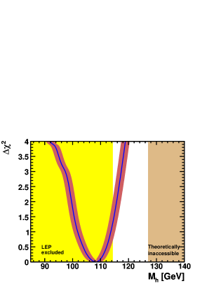
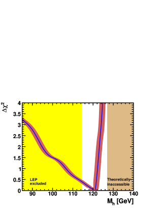
Figure 15: The $\chi^{2}$ functions for $M_{h}$ in the CMSSM (left) and the NUHM1 (right) [74], including the theoretical uncertainties (red bands). Also shown is the mass range excluded for a SM-like Higgs boson (yellow shading), and the ranges theoretically inaccessible in the supersymmetric models studied.

In the case of the CMSSM, we see in the left panel of Figure 15 that the minimum of the $\chi^{2}$ function occurs below the LEP exclusion limit. The fit result is still compatible at the 95% C.L. with the search limit, similarly to the SM case. In the case of the NUHM1, shown in the right panel of Fig. 15, we see that the minimum of the $\chi^{2}$ function occurs above the LEP lower limit on the mass of a SM Higgs. Thus, within the NUHM1 the combination of all other experimental constraints naturally evades the LEP Higgs constraints, and no tension between $M_{h}$ and the experimental bounds exists.

Acknowledgments

I thank the organizers for their hospitality and for creating a very stimulating environment, as well as, together with the participants, for an exceptionally nice school dinner/farewell party.

References

References

- [1] P. W. Higgs, Phys. Lett. 12 (1964) 132; Phys. Rev. Lett. 13 (1964) 508; Phys. Rev. 145 (1966) 1156;
- [2] F. Englert and R. Brout, Phys. Rev. Lett. 13 (1964) 321;
- [3] G. S. Guralnik, C. R. Hagen and T. W. B. Kibble, Phys. Rev. Lett. 13 (1964) 585.
-
[4]
S.L. Glashow,
Nucl. Phys. B 22 (1961) 579;
S. Weinberg, Phys. Rev. Lett. 19 (1967) 19;
A. Salam, in: Proceedings of the 8th Nobel Symposium, Editor N. Svartholm, Stockholm, 1968. -
[5]
H. Nilles,
Phys. Rept. 110 (1984) 1;
H. Haber and G. Kane, Phys. Rept. 117 (1985) 75;
R. Barbieri, Riv. Nuovo Cim. 11 (1988) 1. -
[6]
S. Weinberg,
Phys. Rev. Lett. 37 (1976) 657;
J. Gunion, H. Haber, G. Kane and S. Dawson, The Higgs Hunter’s Guide (Perseus Publishing, Cambridge, MA, 1990), and references therein. -
[7]
P. Fayet,
Nucl. Phys. B 90 (1975) 104;
Phys. Lett. B 64 (1976) 159;
Phys. Lett. B 69 (1977) 489;
Phys. Lett. B 84 (1979) 416;
H.P. Nilles, M. Srednicki and D. Wyler, Phys. Lett. B 120 (1983) 346;
J.M. Frere, D.R. Jones and S. Raby, Nucl. Phys. B 222 (1983) 11;
J.P. Derendinger and C.A. Savoy, Nucl. Phys. B 237 (1984) 307;
J. Ellis, J. Gunion, H. Haber, L. Roszkowski and F. Zwirner, Phys. Rev. D 39 (1989) 844;
M. Drees, Int. J. Mod. Phys. A 4 (1989) 3635. -
[8]
N. Arkani-Hamed, A. Cohen and H. Georgi,
Phys. Lett. B 513 (2001) 232
[arXiv:hep-ph/0105239];
N. Arkani-Hamed, A. Cohen, T. Gregoire and J. Wacker, JHEP 0208 (2002) 020 [arXiv:hep-ph/0202089]. -
[9]
N. Arkani-Hamed, S. Dimopoulos and G. Dvali,
Phys. Lett. B 429 (1998) 263
[arXiv:hep-ph/9803315];
Phys. Lett. B 436 (1998) 257
[arXiv:hep-ph/9804398];
I. Antoniadis, Phys. Lett. B 246 (1990) 377;
J. Lykken, Phys. Rev. D 54 (1996) 3693 [arXiv:hep-th/9603133];
L. Randall and R. Sundrum, Phys. Rev. Lett. 83 (1999) 3370 [arXiv:hep-ph/9905221]. - [10] G. Weiglein et al. [LHC/ILC Study Group], Phys. Rept. 426 (2006) 47 [arXiv:hep-ph/0410364].
- [11] A. De Roeck et al., arXiv:0909.3240 [hep-ph].
-
[12]
N. Cabibbo, L. Maiani, G. Parisi and R. Petronzio,
Nucl. Phys. B 158 (1979) 295;
R. Flores and M. Sher, Phys. Rev. D 27 (1983) 1679;
M. Lindner, Z. Phys. C 31 (1986) 295;
M. Sher, Phys. Rept. 179 (1989) 273;
J. Casas, J. Espinosa and M. Quiros, Phys. Lett. 342 (1995) 171. [arXiv:hep-ph/9409458]. - [13] G. Altarelli and G. Isidori, Phys. Lett. B 337 (1994) 141; J. Espinosa and M. Quiros, Phys. Lett. 353 (1995) 257 [arXiv:hep-ph/9504241].
- [14] T. Hambye and K. Riesselmann, Phys. Rev. D 55 (1997) 7255 [arXiv:hep-ph/9610272].
- [15] T. Hahn, S. Heinemeyer, F. Maltoni, G. Weiglein and S. Willenbrock, arXiv:hep-ph/0607308.
- [16] G. Aad et al. [The ATLAS Collaboration], arXiv:0901.0512.
- [17] G. Bayatian et al. [CMS Collaboration], J. Phys. G 34 (2007) 995.
-
[18]
LEP Electroweak Working Group,
see: lepewwg.web.cern.ch/LEPEWWG/Welcome.html . - [19] Tevatron Electroweak Working Group, see: tevewwg.fnal.gov .
-
[20]
The ALEPH, DELPHI, L3, OPAL, SLD Collaborations,
the LEP Electroweak Working Group,
the SLD Electroweak and Heavy Flavour Groups,
Phys. Rept. 427 (2006) 257
[arXiv:hep-ex/0509008];
[The ALEPH, DELPHI, L3 and OPAL Collaborations, the LEP Electroweak Working Group], arXiv:hep-ex/0612034. - [21] A. Sirlin, Phys. Rev. D 22 (1980) 971; W. Marciano and A. Sirlin, Phys. Rev. D 22 (1980) 2695.
- [22] M. Veltman, Nucl. Phys. B 123 (1977) 89.
- [23] LEP Higgs working group, Phys. Lett. B 565 (2003) 61 [arXiv:hep-ex/0306033].
- [24] ALEPH Collaboration, CDF Collaboration, D0 Collaboration, DELPHI Collaboration, L3 Collaboration, OPAL Collaboration, SLD Collaboration, LEP Electroweak Working Group, Tevatron Electroweak Working Group, SLD electroweak heavy flavour groups, arXiv:0911.2604 [hep-ex].
- [25] Tevatron Electroweak Working Group and CDF Collaboration and D0 Collaboration, arXiv:0903.2503 [hep-ex].
- [26] M. Grünewald, arXiv:0709.3744 [hep-ex]; arXiv:0710.2838 [hep-ex].
- [27] M. Grünewald, priv. communication.
- [28] G. Montagna, O. Nicrosini, F. Piccinini and G. Passarino, Comput. Phys. Commun. 117 (1999) 278 [arXiv:hep-ph/9804211].
- [29] D. Bardin et al., Comput. Phys. Commun. 133 (2001) 229 [arXiv:hep-ph/9908433]; A. Arbuzov et al., Comput. Phys. Commun. 174 (2006) 728 [arXiv:hep-ph/0507146].
- [30] [CDF Collaboration and D0 Collaboration], arXiv:0903.4001 [hep-ex].
-
[31]
H. Flacher, M. Goebel, J. Haller, A. Hocker, K. Moenig
and J. Stelzer,
Eur. Phys. J. C 60 (2009) 543
[arXiv:0811.0009 [hep-ph]];
see: cern.ch/gfitter . - [32] [CDF Collaboration and D0 Collaboration], arXiv:0911.3930 [hep-ex].
- [33] U. Baur, R. Clare, J. Erler, S. Heinemeyer, D. Wackeroth, G. Weiglein and D. Wood, arXiv:hep-ph/0111314.
-
[34]
J. Erler, S. Heinemeyer, W. Hollik, G. Weiglein
and P. Zerwas,
Phys. Lett. B 486 (2000) 125
[arXiv:hep-ph/0005024];
J. Erler and S. Heinemeyer, arXiv:hep-ph/0102083. - [35] R. Hawkings and K. Mönig, EPJdirect C8 (1999) 1 [arXiv:hep-ex/9910022].
- [36] G. Wilson, LC-PHSM-2001-009, see: www.desy.de/lcnotes/notes.html.
- [37] S. Heinemeyer et al., arXiv:hep-ph/0511332.
- [38] S. Glashow and S. Weinberg, Phys. Rev. D 15 (1977) 1958.
- [39] C. Amsler et al. [Particle Data Group], Phys. Lett. B 667 (2008) 1.
- [40] A. Djouadi, Phys. Rept. 459 (2008) 1 [arXiv:hep-ph/0503173].
- [41] J. Gunion, H. Haber, G. Kane and S. Dawson, The Higgs Hunter’s Guide, Addison-Wesley, 1990.
- [42] S. Heinemeyer, Int. J. Mod. Phys. A 21 (2006) 2659 [arXiv:hep-ph/0407244].
- [43] LEP Higgs working group, Eur. Phys. J. C 47 (2006) 547 [arXiv:hep-ex/0602042].
-
[44]
J. Ellis, G. Ridolfi and F. Zwirner,
Phys. Lett. B 257 (1991) 83;
Y. Okada, M. Yamaguchi and T. Yanagida, Prog. Theor. Phys. 85 (1991) 1;
H. Haber and R. Hempfling, Phys. Rev. Lett. 66 (1991) 1815. - [45] A. Brignole, Phys. Lett. B 281 (1992) 284.
- [46] P. Chankowski, S. Pokorski and J. Rosiek, Phys. Lett. B 286 (1992) 307; Nucl. Phys. B 423 (1994) 437, hep-ph/9303309.
- [47] A. Dabelstein, Nucl. Phys. B 456 (1995) 25, hep-ph/9503443; Z. Phys. C 67 (1995) 495, hep-ph/9409375.
- [48] R. Hempfling and A. Hoang, Phys. Lett. B 331 (1994) 99, hep-ph/9401219.
- [49] S. Heinemeyer, W. Hollik and G. Weiglein, Phys. Rev. D 58 (1998) 091701, hep-ph/9803277; Phys. Lett. B 440 (1998) 296, hep-ph/9807423.
- [50] S. Heinemeyer, W. Hollik and G. Weiglein, Eur. Phys. Jour. C 9 (1999) 343, hep-ph/9812472.
-
[51]
R. Zhang, Phys. Lett. B 447 (1999) 89,
hep-ph/9808299;
J. Espinosa and R. Zhang, JHEP 0003 (2000) 026, hep-ph/9912236. - [52] G. Degrassi, P. Slavich and F. Zwirner, Nucl. Phys. B 611 (2001) 403, hep-ph/0105096.
- [53] J. Espinosa and R. Zhang, Nucl. Phys. B 586 (2000) 3, hep-ph/0003246.
- [54] A. Brignole, G. Degrassi, P. Slavich and F. Zwirner, Nucl. Phys. B 631 (2002) 195, hep-ph/0112177.
- [55] A. Brignole, G. Degrassi, P. Slavich and F. Zwirner, Nucl. Phys. B 643 (2002) 79, hep-ph/0206101.
- [56] S. Heinemeyer, W. Hollik, H. Rzehak and G. Weiglein, Eur. Phys. J. C 39 (2005) 465 [arXiv:hep-ph/0411114].
-
[57]
T. Banks,
Nucl. Phys. B 303 (1988) 172;
L. Hall, R. Rattazzi and U. Sarid, Phys. Rev. D 50 (1994) 7048, hep-ph/9306309;
R. Hempfling, Phys. Rev. D 49 (1994) 6168;
M. Carena, M. Olechowski, S. Pokorski and C. Wagner, Nucl. Phys. B 426 (1994) 269, hep-ph/9402253. - [58] M. Carena, D. Garcia, U. Nierste and C. Wagner, Nucl. Phys. B 577 (2000) 577, hep-ph/9912516.
- [59] G. Degrassi, A. Dedes and P. Slavich, Nucl. Phys. B 672 (2003) 144, hep-ph/0305127.
-
[60]
S. Martin,
Phys. Rev. D 65 (2002) 116003
[arXiv:hep-ph/0111209];
Phys. Rev. D 66 (2002) 096001
[arXiv:hep-ph/0206136];
Phys. Rev. D 67 (2003) 095012
[arXiv:hep-ph/0211366];
Phys. Rev. D 68 (2003) 075002
[arXiv:hep-ph/0307101];
Phys. Rev. D 70 (2004) 016005
[arXiv:hep-ph/0312092];
Phys. Rev. D 71 (2005) 016012
[arXiv:hep-ph/0405022];
Phys. Rev. D 71 (2005) 116004
[arXiv:hep-ph/0502168];
Phys. Rev. D 75 (2007) 055005
[arXiv:hep-ph/0701051];
S. Martin and D. Robertson, Comput. Phys. Commun. 174 (2006) 133 [arXiv:hep-ph/0501132]. - [61] R. Harlander, P. Kant, L. Mihaila and M. Steinhauser, Phys. Rev. Lett. 100 (2008) 191602 [Phys. Rev. Lett. 101 (2008) 039901] [arXiv:0803.0672 [hep-ph]].
- [62] G. Degrassi, S. Heinemeyer, W. Hollik, P. Slavich and G. Weiglein, Eur. Phys. J. C 28 (2003) 133 [arXiv:hep-ph/0212020].
- [63] S. Heinemeyer, W. Hollik and G. Weiglein, Comput. Phys. Commun. 124 (2000) 76 [arXiv:hep-ph/9812320]; see: www.feynhiggs.de .
- [64] M. Frank, T. Hahn, S. Heinemeyer, W. Hollik, H. Rzehak and G. Weiglein, JHEP 0702 (2007) 047 [arXiv:hep-ph/0611326].
- [65] M. Diaz and H. Haber, Phys. Rev. D 45 (1992) 4246.
- [66] M. Frank, PhD thesis, university of Karlsruhe, 2002.
- [67] M. Carena, S. Heinemeyer, C. Wagner and G. Weiglein, Eur. Phys. J. C 26 (2003) 601 [arXiv:hep-ph/0202167].
- [68] M. Carena, S. Heinemeyer, C. Wagner and G. Weiglein, Eur. Phys. J. C 45 (2006) 797 [arXiv:hep-ph/0511023].
- [69] S. Gennai, S. Heinemeyer, A. Kalinowski, R. Kinnunen, S. Lehti, A. Nikitenko and G. Weiglein, Eur. Phys. J. C 52 (2007) 383 [arXiv:0704.0619 [hep-ph]]; M. Hashemi, S. Heinemeyer, R. Kinnunen, A. Nikitenko and G. Weiglein, arXiv:0804.1228 [hep-ph].
- [70] S. Heinemeyer, W. Hollik, D. Stockinger, A. M. Weber and G. Weiglein, JHEP 0608 (2006) 052 [arXiv:hep-ph/0604147].
- [71] S. Heinemeyer, W. Hollik and G. Weiglein, Phys. Rept. 425 (2006) 265 [arXiv:hep-ph/0412214].
- [72] O. Buchmueller et al., Phys. Lett. B 657 (2007) 87 [arXiv:0707.3447 [hep-ph]].
- [73] O. Buchmueller et al., JHEP 0809 (2008) 117 [arXiv:0808.4128 [hep-ph]].
- [74] O. Buchmueller et al., Eur. Phys. J. C 64 (2009) 391 [arXiv:0907.5568 [hep-ph]].
- [75] See: cern.ch/mastercode .
- [76] B. Allanach, Comput. Phys. Commun. 143 (2002) 305 [arXiv:hep-ph/0104145].
- [77] T. Moroi, Phys. Rev. D 53 (1996) 6565 [Erratum-ibid. D 56 (1997) 4424] [arXiv:hep-ph/9512396].
- [78] G. Degrassi and G. F. Giudice, Phys. Rev. D 58 (1998) 053007 [arXiv:hep-ph/9803384].
- [79] S. Heinemeyer, D. Stockinger and G. Weiglein, Nucl. Phys. B 690 (2004) 62 [arXiv:hep-ph/0312264].
- [80] S. Heinemeyer, D. Stockinger and G. Weiglein, Nucl. Phys. B 699 (2004) 103 [arXiv:hep-ph/0405255].
- [81] S. Heinemeyer, W. Hollik, A. M. Weber and G. Weiglein, JHEP 0804 (2008) 039 [arXiv:0710.2972 [hep-ph]].
- [82] G. Isidori and P. Paradisi, Phys. Lett. B 639 (2006) 499 [arXiv:hep-ph/0605012].
- [83] G. Isidori, F. Mescia, P. Paradisi and D. Temes, Phys. Rev. D 75 (2007) 115019 [arXiv:hep-ph/0703035], and references therein.
- [84] F. Mahmoudi, Comput. Phys. Commun. 178 (2008) 745 [arXiv:0710.2067 [hep-ph]]; Comput. Phys. Commun. 180 (2009) 1579 [arXiv:0808.3144 [hep-ph]].
- [85] D. Eriksson, F. Mahmoudi and O. Stal, JHEP 0811 (2008) 035 [arXiv:0808.3551 [hep-ph]].
- [86] G. Belanger, F. Boudjema, A. Pukhov and A. Semenov, Comput. Phys. Commun. 176 (2007) 367 [arXiv:hep-ph/0607059]; Comput. Phys. Commun. 149 (2002) 103 [arXiv:hep-ph/0112278]; Comput. Phys. Commun. 174 (2006) 577 [arXiv:hep-ph/0405253].
- [87] P. Gondolo, J. Edsjo, P. Ullio, L. Bergstrom, M. Schelke and E. Baltz, New Astron. Rev. 49 (2005) 149; JCAP 0407 (2004) 008 [arXiv:astro-ph/0406204].
- [88] P. Skands et al., JHEP 0407 (2004) 036 [arXiv:hep-ph/0311123].
- [89] B. Allanach et al., Comput. Phys. Commun. 180 (2009) 8 [arXiv:0801.0045 [hep-ph]].
- [90] LEP Supersymmetry Working Group, see: lepsusy.web.cern.ch/lepsusy/ .