Multiple vortex-antivortex pair generation in magnetic nanodots

Abstract

The interaction of a magnetic vortex with a rotating magnetic field causes the nucleation of a vortex–antivortex pair leading to a vortex polarity switching. The key point of this process is the creation of a dip, which can be interpreted as a nonlinear resonance in the system of certain magnon modes with nonlinear coupling. The usually observed single-dip structure is a particular case of a multidip structure. The dynamics of the structure with $n$ dips is described as the dynamics of nonlinearly coupled modes with azimuthal numbers $m=0,\pm n,\pm 2n$. The multidip structure with arbitrary number of vortex-antivortex pairs can be obtained in vortex-state nanodisk using a space- and time-varying magnetic field. A scheme of a possible experimental setup for multidip structure generation is proposed.

I Introduction

A magnetization curling occurs in magnetic particles of nanoscale due to the dipole-dipole interaction. In particular, the vortex state is realized in a disk shaped particle, where the magnetization becomes circular lying in the disk plane in the main part of the sample, which possesses a flux-closure state. At the disk center there appears an out-of-plane magnetization structure (the vortex core, typically from 10 nm Wachowiak et al. (2002) to 23 nm Chou et al. (2007)) due to the dominant role of the exchange interaction inside the core. Hubert and Schäfer (1998); Skomski (2003) The vortex state of magnetic nanodots has drawn much attention because it could be used for high-density magnetic storage and miniature sensors. Cowburn (2002); Skomski (2003) Apart from that, such nanodots are very attractive objects for experimental investigation of the vortex dynamics on a nanoscale.

An experimental discovery of a vortex core reversal process by excitation with short bursts of an alternating field Van Waeyenberge et al. (2006) initiated a number of studies of the core switching process. The mechanism of the vortex switching is of general nature; it is essentially the same in all systems where the switching was observed. Van Waeyenberge et al. (2006); Xiao et al. (2006); Hertel et al. (2007); Lee et al. (2007); Yamada et al. (2007); Kravchuk et al. (2007); Sheka et al. (2007); Liu et al. (2007); Vansteenkiste et al. (2009); Weigand et al. (2009) There are two main stages of the switching process: (i) At the first stage of the process the vortex structure is excited by the pumping, leading to the creation of an out–of–plane dip with opposite sign nearby the vortex. The appearance of such a deformation is confirmed experimentally. Vansteenkiste et al. (2009); Weigand et al. (2009) (ii) At the second stage, when the dip amplitude reaches the maximum possible value, there appears a vortex–antivortex pair from the dip structure. The further dynamics is accompanied by the annihilation of the original vortex with the new antivortex, leading effectively to the switching of the vortex polarity; the dynamics of this three body problem can be described analytically. Gaididei et al. (2008, 2010) While the second stage is well understood, the physical picture of the first stage of the switching process, which is a dip creation, is still not clear.

The aim of the current study is to develop a theory of the dip creation, which is a key moment in the vortex switching process. The dip always appears as a nonlinear regime of one of the magnon modes. In most studies the dip appears by exciting a low frequency gyromode, which corresponds to the azimuthal quantum number $m=-1$; the frequency of this mode $\omega_{G}$ lies in the sub GHz range. Excitation of the gyromode always leads to a macrospopic motion of the vortex as a whole; moreover the vortex has to reach some critical velocity $v_{\text{cri}}$ of about 300 m/s in order to switch its polarity Lee et al. (2008); Vansteenkiste et al. (2008).

Recently we have reported about vortex core switching under the action of a homogeneous rotating magnetic field $\bm{B}=B_{x}+iB_{y}=B_{0}\exp(i\omega t)$. Kravchuk et al. (2007) The theory of the dip creation was constructed very recently in our previous paper Kravchuk et al. (2009), where we found a dip as a nonlinear regime of the high frequency mode with $m=1$; the switching process for that case is not accompanied by a vortex motion at all. In this paper we show that the dip can be excited for any azimuthal mode $m$ by using a nonhomogeneous rotating magnetic field of the form (16).

The paper is organized as follows. In Sec. II we formulate the model and describe the approach of a rotating reference frame. Two kinds of numerical simulations are presented in Sec. III: micromagnetic OOMMF simulations (Sec. III.1) and spin–lattice SLASI simulations in the rotating frame (Sec. III.2). An analytical approach is presented in Sec. IV. We discuss our results in Sec. V. In Appendix A we prove the conservation law for the total momentum $J_{z}$ under the action of the magnetostatic interaction. A possible experimental setup for multidip structure generation is discussed in Appendix B.

II Model and continuum description

The continuum dynamics of the the spin system can be described in terms of the magnetization unit vector $\bm{m}=\bm{M}/M_{S}=\left(\sin\vartheta\cos\varphi,\sin\vartheta\sin\varphi,\cos\vartheta\right)$, where $\vartheta$ and $\varphi$ are functions of the coordinates and the time, and $M_{S}$ is the saturation magnetization. In the subsequent text only disk shaped samples are discussed. Therefore it is convenient to introduce dimensionless coordinates $\bm{\rho}=(x,y)/L$ within the disk plane and $\zeta=z/h$ along the disk axis, where $L$ is the disk radius and $h$ is its thickness. The magnetization is assumed to be uniform along the $z$-axis and so the corresponding angular coordinates of the magnetization read $\theta(\bm{\rho})=\vartheta(L\bm{\rho})$ and $\phi(\bm{\rho})=\varphi(L\bm{\rho})$. The energy functional of the system under consideration consists of three terms,

$$E=4\pi M_{S}^{2}V\left(\mathscr{E}^{\text{ex}}+\mathscr{E}^{\text{ms}}+\mathscr{E}^{\text{f}}\right).$$ (1)

Here $V$ is volume of the sample. The dimensionless energy terms are the following:

$$\mathscr{E}^{\text{ex}}=\frac{1}{2\pi}\frac{\ell^{2}}{L^{2}}\int\!\mathrm{d}^{2}\bm{\rho}\left[\left(\nabla\theta\right)^{2}+\sin^{2}\theta\left(\nabla\phi\right)^{2}\right]$$ (2)

is the exchange energy with $\ell=\sqrt{A/4\pi M_{S}^{2}}$ being the exchange length, $A$ being the exchange constant. The magnetostatic energy $\mathscr{E}^{\text{ms}}$ comes from the dipolar interaction, see Appendix A, and in the continuum limit it can be presented as a sum of three terms: $\mathscr{E}^{\text{ms}}=\mathscr{E}_{\text{v}}^{\text{ms}}+\mathscr{E}_{\text{s}}^{\text{ms}}+\mathscr{E}_{\text{e}}^{\text{ms}}$. Here

$$\mathscr{E}_{\text{v}}^{\text{ms}}=\frac{\varepsilon}{4\pi^{2}}\int_{\mathcal{V}}\!\mathrm{d}\mathcal{V}\int_{\mathcal{V}^{\prime}}\!\mathrm{d}\mathcal{V}^{\prime}\frac{\nabla\!\cdot\!\bm{m}(\bm{\rho})\nabla\!\cdot\!\bm{m}(\bm{\rho}^{\prime})}{\sqrt{(\bm{\rho}-\bm{\rho}^{\prime})^{2}+(\zeta-\zeta^{\prime})^{2}}}$$ (3)

is the energy of the interactions of volume magnetostatic charges, where $\varepsilon=h/L$ is the disk aspect ratio and $\int_{\mathcal{V}}\mathrm{d}\mathcal{V}=\int_{0}^{1}\mathrm{d}\zeta\int_{0}^{1}\mathrm{d}\rho\rho\int_{0}^{2\pi}\mathrm{d}\chi$ with $(\rho,\chi)$ being polar coordinates within the disk plane.

$$\begin{split}\mathscr{E}_{\text{s}}^{\text{ms}}=\frac{1}{2\pi^{2}\varepsilon}\int_{\mathcal{S}}\!\mathrm{d}\mathcal{S}\int_{\mathcal{S}^{\prime}}\!&\mathrm{d}\mathcal{S}^{\prime}\cos\theta(\bm{\rho})\cos\theta(\bm{\rho}^{\prime})\times\\ &\left[\frac{1}{|\bm{\rho}-\bm{\rho}^{\prime}|}-\frac{1}{\sqrt{(\bm{\rho}-\bm{\rho}^{\prime})^{2}+\varepsilon^{2}}}\right]\end{split}$$ (4)

is the energy of the interactions of charges on the upper and bottom surfaces, where $\int_{\mathcal{S}}\mathrm{d}\mathcal{S}=\int_{0}^{1}\mathrm{d}\rho\rho\int_{0}^{2\pi}\mathrm{d}\chi$.

$$\mathscr{E}_{\text{e}}^{\text{ms}}=-\frac{\varepsilon}{2\pi^{2}}\int_{\mathcal{V}}\!\mathrm{d}\mathcal{V}\int_{\Sigma^{\prime}}\!\mathrm{d}\Sigma^{\prime}\frac{\nabla\!\cdot\!\bm{m}(\bm{\rho})\cos[\phi(\bm{\rho}^{\prime})-\chi^{\prime}]}{\sqrt{(\bm{\rho}-\bm{\rho}^{\prime})^{2}+(\zeta-\zeta^{\prime})^{2}}}$$ (5)

is the energy of the interactions of edge surface charges with the volume charges. Here $\Sigma$ is the disk edge surface and $\int_{\Sigma}\mathrm{d}\Sigma=\int_{0}^{1}\mathrm{d}\zeta\int_{0}^{2\pi}\mathrm{d}\chi$. Due to magnetization uniformity along the $z$-axis the distribution of upper and bottom surface charges is antisymmetrical and the distributions of volume and edge surface charges are uniform along the $z$-axis. As a result the interaction energy of upper and bottom surface charges with volume charges as well as with edge surface charges is equal to zero. The last term in (1) describes an interaction with a nonhomogeneous rotating magnetic field, see below.

The evolution of magnetization can be described by the Landau–Lifshitz–Gilbert (LLG) equation:

$$-\sin\theta\ \dot{\phi} =-\pi\frac{\delta\mathscr{E}}{\delta\theta}-\eta\dot{\theta},$$ (6a)

$$\sin\theta\ \dot{\theta} =-\pi\frac{\delta\mathscr{E}}{\delta\phi}-\eta\sin^{2}\theta\dot{\phi}.$$ (6b)

Here and below the overdot indicates derivative with respect to the dimensionless time

$$\tau=\omega_{0}t,\qquad\omega_{0}=4\pi\gamma M_{S},$$ (7)

where $\gamma$ is the gyromagnetic ratio, $\eta$ is the Gilbert damping constant, and the factor $\pi$ appears due to the disk volume normalization. These equations can be derived from the following Lagrangian

$$\mathscr{L}=\frac{1}{\pi}\int\!\mathrm{d}^{2}\bm{\rho}\left(1-\cos\theta\right)\dot{\phi}-\mathscr{E}$$ (8)

and dissipation function

$$\mathscr{F}=\frac{\eta}{2\pi}\int\!\mathrm{d}^{2}\bm{\rho}\left({\dot{\theta}}^{2}+\sin^{2}\theta{\dot{\phi}}^{2}\right).$$ (9)

Let us start with the no–driving case $\mathscr{E}^{\mathrm{f}}=0$. The exchange interaction (2) provides the conservation of the total magnetization $M_{z}$ along the cylindrical axis $z$ and the conservation of the $z$–component of the orbital momentum $L_{z}$

$$M_{z}=\frac{1}{\pi}\int\!\mathrm{d}^{2}\bm{\rho}\cos\theta,\qquad L_{z}=-\frac{1}{\pi}\int\!\mathrm{d}^{2}\bm{\rho}\cos\theta\partial_{\chi}\phi$$ (10)

due to the invariance under rotation about the $z$-axis in spin-space and physical space, respectively. It is well–knownPapanicolaou and Tomaras (1991) that the magnetostatic interaction breaks both symmetries. Nevertheless for thin cylindrical samples, when the magnetization distribution does not depend on the thickness coordinate, the magnetostatic energy is invariant under two simultaneous rotations

$$\phi\rightarrow\phi+\varphi_{0},\qquad\chi\rightarrow\chi+\varphi_{0},$$ (11)

leading to the conservation of the total momentum

$$J_{z}=\frac{1}{\pi}\int\!\mathrm{d}^{2}\bm{\rho}\left(\cos\theta-1\right)\left(1-\partial_{\chi}\phi\right),$$ (12)

see the proof in Appendix A.

II.1 Planar vortex and magnon modes

The ground state of a small size nanodisk is uniform; it depends on the particle aspect ratio $\varepsilon$: thin nanodisks are magnetized in the plane (when $\varepsilon<\varepsilon_{c}\approx 1.812$) and thick ones along the axis (when $\varepsilon>\varepsilon_{c}$). When the particle size exceeds some critical value, the magnetization curling becomes energetically preferable due to the competition between the exchange and dipolar interaction. For a disk shape particle there appears the vortex state.

Let us consider the static solutions of the Landau-Lifshitz equation with in–plane magnetization ($\theta\equiv\pi/2$). The in-plane magnetization angle $\phi$ satisfies the Laplace equation $\nabla^{2}\phi=0$. Typically for the Heisenberg magnets the boundary is free, which corresponds to the Neumann boundary conditions. However, the dipolar interaction orients the magnetization tangentially to the boundary in order to decrease the surface charges. Effectively this can be described by fixed (Dirichlet) boundary conditions. The simplest topologically nontrivial solution of this boundary value problem is the planar vortex, situated at the disk center

$$\phi^{\text{v}}=\chi+\mathfrak{C}\frac{\pi}{2},$$ (13)

where $\mathfrak{C}=\pm 1$ is the vortex chirality. Such planar vortices are known for the Heisenberg magnets with strong enough easy–plane anisotropy Mertens and Bishop (2000). Qualitatively, when the typical magnetic length is smaller than the lattice constant, the pure planar vortex can be realized. In the magnetically soft nanomagnets like permalloy, there exist out–of–plane vortices. The typical out–of–plane vortex structure has a bell–shaped form with a core size about the exchange length. Hubert and Schäfer (1998)

Magnons on a vortex background can be described using the partial wave expansion:

$$\begin{split}\cos\theta&=\cos\theta^{\text{v}}(\rho)+\frac{1}{\sqrt{2}}\sum_{m,n}\alpha_{m,n}(\tau)f_{|m|,n}(\rho)e^{im\chi},\\ \phi&=\phi^{\text{v}}+\frac{1}{\sqrt{2}}\sum_{m,n}\beta_{m,n}(\tau)g_{|m|,n}(\rho)e^{im\chi},\end{split}$$ (14)

where $\alpha_{m,n}=\alpha_{-m,n}^{\star}$ and $\beta_{m,n}=\beta_{-m,n}^{\star}$. In the linear regime $\alpha_{m,n}(\tau)=\exp(i\varOmega_{m,n}\tau)$ and $\beta_{m,n}(\tau)=\exp(i\varOmega_{m,n}\tau)$. We consider here the planar vortex, where the spectrum of eigenmodes is degenerate with respect to the sign of $m$. Typical eigenfrequencies are presented in Fig. 1. The functions $f$ and $g$ obey the following normalization rule

$$\langle f_{m,n}g_{m^{\prime},n^{\prime}}\rangle\equiv\int_{0}^{1}f_{m,n}(\rho)g_{m^{\prime},n^{\prime}}(\rho)\rho\mathrm{d}\rho=\delta_{m,m^{\prime}}\delta_{n,n^{\prime}}.$$ (15)

Below we assume that for each azimuthal number $m$ it is sufficient to take into account only one radial wave with a certain radial index $n$. Therefore the summation over $n$ will be omitted.

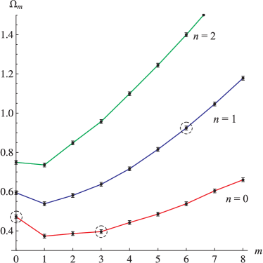
Figure 1: (Color online) Eigenfrequencies of the magnon waves in a vortex-state Py disk ($150$ nm diameter, $20$ nm thickness). The spectrum was obtained using micromagnetic modelling with a fixed in–plane vortex core (for technical details see Sec. III). The frequencies are normalized by $\omega_{0}=4\pi\gamma M_{S}$ (30.3 GHz). $n$ denotes the radial wave number – the number of roots of the functions $f(\rho)$ and $g(\rho)$. The separation of waves with different $m$ and $n$ was achieved using spatio-temporal Fourier transform technique.

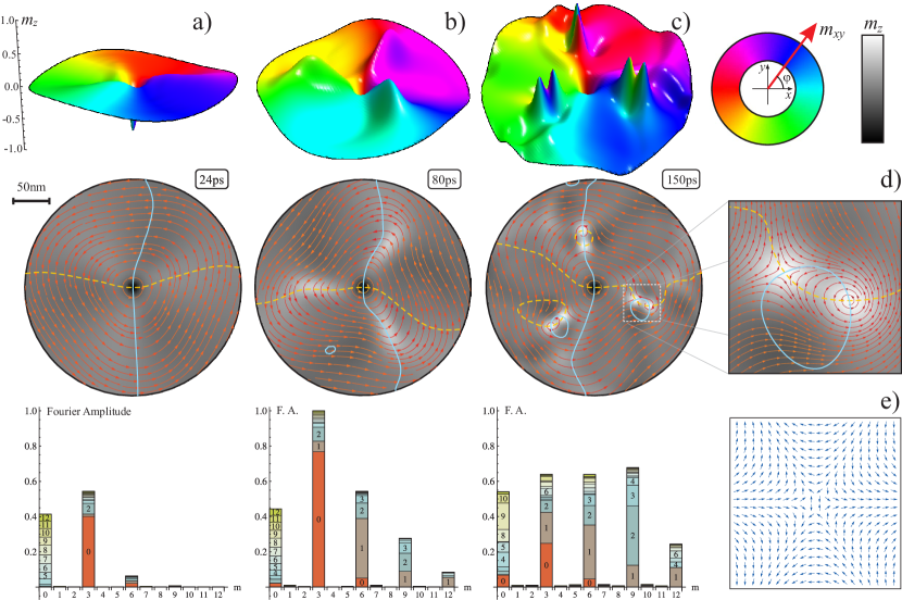
Figure 2: (Color online) Vortex state dynamics under influence of the field (16) with $\mu=-3$, $B_{0}$=40mT and $\omega$=6GHz. Disk radius $L$=150nm. Columns a), b) and c) correspond to the different moments of time after the field switching-on moment: 24, 80 and 150ps, respectively. The top row of these columns illustrates distribution of the out-of-plane magnetization component ($m_{z}$). The in-plane component distribution is shown in the second row. Isolines $m_{x}=0$ and $m_{y}=0$ are shown as dashed and solid lines, respectively. In the bottom row the corresponding two-dimensional spatial Fourier transforms of the distribution $m_{z}(r,\chi)$ are presented. Each bar of a certain color corresponds to a Fourier amplitude $F_{mn}$, where the azimuthal wave number $m$ is specified by the horizontal axis and the radial number $n$ is indicated on the bar. The subfig. d) demonstrates a vortex-antivortex pair in detail. The used magnetic field at $t=0$ is shown in the subfig. e).

II.2 Interaction with a field

Let us consider the effects of a magnetic field. The role of the field is to excite spin waves on a vortex background. It is well known that the low frequency gyroscopical mode can be excited by applying a homogeneous ac field with a frequency $\omega_{G}$ in the sub GHz range. The strong pumping of such a mode is known to cause the vortex polarity switching.

The vortex switching phenomenon was studied recently by applying a homogeneous high frequency rotating magnetic field.Kravchuk et al. (2009) Such a field excites the azimuthal mode with azimuthal number $m=\pm 1$; the frequency $\omega_{1}$ of such a mode lies in the range of 10 GHz.Kravchuk et al. (2007)

In the present work we study the vortex switching process by exciting higher magnon modes with higher azimuthal numbers $m$. In order to excite such a mode we propose to consider the influence of a nonhomogeneous rotating magnetic field

$$\bm{B}=B_{x}+iB_{y}=B_{0}e^{i(\mu+1)\chi+i\omega t},\qquad\mu\in\mathbb{Z}.$$ (16)

Such a field distribution is chosen, because it directly pumps the magnon mode with $m=\mu$. Using Ansatz (14) one can easily calculate the Zeeman energy

$$\begin{split}\mathscr{E}^{\text{f}}&=-\frac{b}{\pi}\int\!\mathrm{d}^{2}\bm{\rho}\sin\theta\cos\Bigl{(}(\mu+1)\chi+\Omega\tau-\phi\Bigr{)}\\ &=b_{e}\left(\beta_{\mu}e^{-i\Omega\tau}+\beta_{\mu}^{\star}e^{i\Omega\tau}\right),\quad b_{e}=\frac{b\mathfrak{C}}{\sqrt{2}}\langle g_{\mu}\rangle.\end{split}$$ (17)

Here and below we use the normalized field intensity $b=B_{0}/4\pi M_{S}$ and field frequency $\Omega=\omega/\omega_{0}$. For the case $\mu<-1$ the field with structure (16) can be created experimentally, for details see Appendix B.

II.3 Rotating frame of reference

In the laboratory frame of reference the total energy $\mathscr{E}$ depends explicitly on time because of the Zeeman term (17), which contains the explicit time dependence. But using a transition into rotating reference frame (RRF) by the way of

$$\widetilde{\phi}=\phi+\widetilde{\Omega}\tau,\qquad\widetilde{\chi}=\chi+\widetilde{\Omega}\tau,\qquad\widetilde{\Omega}=\frac{\Omega}{\mu},$$ (18)

and using the invariance of the exchange and magnetostatic energies with respect to the simultaneous rotations (11), we obtain the time-independent energy in the RRF:

$$\widetilde{\mathscr{E}}=\mathscr{E}^{\mathrm{ex}}+\mathscr{E}^{\mathrm{ms}}+\widetilde{\mathscr{E}}^{\mathrm{f}}-\widetilde{\Omega}J_{z}$$ (19)

Here the Zeeman term $\widetilde{\mathscr{E}}^{\mathrm{f}}$ does not contain time explicitly and has the form

$$\widetilde{\mathscr{E}}^{\mathrm{f}}=b_{e}\left(\beta_{\mu}+\beta_{\mu}^{\star}\right).$$ (20)

The dissipation function (9) in the RRF reads

$$\begin{split}\widetilde{\mathscr{F}}&=\mathscr{F}+\widetilde{\Omega}\mathfrak{F},\\ \mathfrak{F}&=\frac{\eta}{\pi}\int\mathrm{d}^{2}\bm{\rho}\left[\dot{\theta}\partial_{\chi}\theta+\sin^{2}\theta(\partial_{\chi}\phi-1)\dot{\phi}\right].\end{split}$$ (21)

III Numerical simulations

To investigate the magnetization dynamics of a vortex state nanodisk under influence of the external magnetic field (16), two kinds of simulations were used.

III.1 Micromagnetic simulations

The main part of the numerical results were obtained using the full scale OOMMF micromagnetic simulations with the material parameters of Permalloy $\mathrm{Ni}_{81}\mathrm{Fe}_{19}$: exchange constant $A=1.3\times 10^{-11}\mathrm{J/m}$, saturation magnetization $M_{S}=8.6\times 10^{5}\mathrm{A/m}$, damping constant $\eta=0.01$. The on-site anisotropy was neglected and the mesh cell was chosen to be $2\mathrm{nm}\times 2\mathrm{nm}\times h$. For all simulations the thickness $h=20\mathrm{nm}$.

An example of magnetization dynamics induced by the field (16) with $\mu=-3$ is explored in Fig. 2.

Initially we have a nanodisk in a vortex state which is a ground state. The vortex polarity was chosen to be negative. During the first tens of picoseconds of the field influence the generation of a magnon mode with azimuthal number $m=-3$ is observed (see column a). The Fourier amplitude which corresponds to $m=0$ appears due to the out-of-plane core component of the initial vortex. Due to the pumping the mode with $m=\mu$ goes to the nonlinear regime: areas with $\mathrm{sign}(m_{z})=\mathrm{sign}(-\mu\omega)$ become localized which can be interpreted as dips formation (see column b). The number of dips is equal to $|\mu|$. For small field amplitudes such a multidip structure achieves some stationary regime and rotates around the vortex center forever. This phenomenon is described in detail below. Fig. 2 demonstrates the example of the magnetization dynamics for larger field amplitudes: the vortex-antivortex pairs are nucleated from the dips (see column c) and subfig. d). The subsequent dynamics of the vortex-antivortex pairs is rather complicated: the trajectory of a pair motion is not circular, pairs radiate magnons during the motion and self-annihilate. Then the process repeats periodically. The question about vortex-antivortex pair motion in the presence of an immobile central vortex is an open problem. But in this paper we focus our attention on the dips creation mechanism only. It should be also emphasized that the initial vortex in Fig. 2 is not pinned but it remains immobile during the dynamics. Using the simulations we found that such a vortex stability is observed only when the number of dips is greater than 2. The theoretical explanation of this phenomenon is an open problem.

Using external fields of the form (16) with different $\mu$ one can obtain a multidip structure with an arbitrary number of dips. This possibility is demonstrated in Fig. 3.

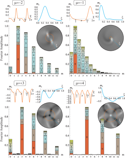
Figure 3: (Color online) Multidip structures created by the field (16) with different $\mu$. To demonstrate the localized character of the dips the distribution of the out-of-plane component $m_{z}$ was obtained along the circle and the line $\xi$ which pass through the extremum points of a multidip structure. The distributions along the circle and the line $\xi$ are shown above Fourier spectra on the left and right plots, respectively. The other notation is the same as in Fig. 2. For the cases $\mu=-2$ and $\mu=-1$ the central vortex core is planar and artificially fixed, for the cases $\mu=+3$ and $\mu=+4$ the central vortex has opposite polarity and is not fixed.

It is important to emphasize the following properties of the multidip structure formation: (i) All dips have the same polarity which is determined by the sign of $m$ only and the dip polarity does not depend neither on the polarity of the central vortex (see the insets for $\mu=+3$ and $\mu=+4$) nor on the existence of an out-of-plane vortex core at all (see the insets for $\mu=-2$ and $\mu=-1$). (ii) the multidip structure with $n$ dips is composed by modes with azimuthal numbers $m=n,\,2n,\,3n,\dots$ The contribution of a mode decreases when its azimuthal number $m$ increases. (iii) Contribution of the mode $m=0$ is essential for a single-dip structure only (compare insets for $\mu=-2$ and $\mu=-1$).

If the strength of the applied field is sufficiently small to prevent vortex-antivortex pair formation, the magnetization dynamics reaches some steady-state regime. This is demonstrated in Fig. 4 a) which is based on simulations with a $\mu=+3$ field. Such a field creates potentially a structure with three dips of negative polarity. The time dependence of the minimal value of the $m_{z}$ component of the azimuthal mode with $m=\mu$ is shown. In case of multidip structures the plotted quantity is the depth of the dips, therefore the notation $m_{z}^{\mathrm{dip}}$ will be used hereafter. One can see that the value $m_{z}^{\mathrm{dip}}$ reaches some steady-state level which depends on the frequency of the applied field. This dependence has an unusual resonance character, see Fig. 4 b).

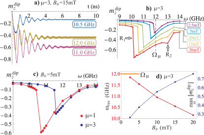
Figure 4: (Color online) Characteristics of the process of multidip structure formation. The data was obtained from simulations with a Py disk with radius $L$=76nm and thickness $h$=20nm. If the multidip structure is formed, then $m_{z}^{\mathrm{dip}}$ denotes the depth of a dip, otherwise it denotes the amplitude of the corresponding azimuthal mode. a) – the process of steady-state three-dips structure formation for a certain field strength and for different frequencies. b) – resonant-type dependencies of the steady-state dips depth on the field frequency for different field amplitudes and for a certain $\mu$. c) – the same as b), but for a certain field amplitude and different $\mu$. d) – data extracted from the resonant curves b): resonant frequency (left axis, solid line) and maximal dips depth (right axis, dashed line) vs applied field amplitude.

The transition from the regime of linear modes to the multidip regime occurs sharply when the frequency of the applied field reaches some value $\omega_{\mathrm{res}}$. Vertical steps on the dependencies $m_{z}^{\mathrm{dip}}(\omega)$ in Fig. 4 b) correspond to the above indicated transition. It should be noted that the critical frequency depends on the field amplitude and is always smaller than the eigenfrequency $\omega_{\mu}$ of the corresponding mode, see Fig. 4 d). This points to an inherently nonlinear nature of the resonance which is discussed in Section IV. Similar resonances are a feature of the multidip structures with different number of dips, Fig. 4 c).

III.2 Spin–lattice simulations

We have described above the micromagnetic study of the nonlinear dynamics of the magnetization under the influence of a time–dependent magnetic field. The main issue of this study is the creation of a multidip structure, i.e. a stable nonlinear state of the system, which rotates due to the field rotation. Since the total energy of the system becomes time independent in the RRF, see (19), one can suppose that a multidip structure forms a stationary state of the system in the RRF.

In order to check the RRF approach, we used another kind of simulations. Namely, we performed SLASI simulations, an in–house–developed spin–lattice code. Caputo et al. (2007) SLASI simulations are based on the numerical solution of the discrete version of the LLG equations (6)

$$\begin{split}\frac{\mathrm{d}\bm{S}_{\bm{n}}}{\mathrm{d}t}=-\left[\bm{S}_{\bm{n}}\times\frac{\partial\mathcal{H}}{\partial\bm{S}_{\bm{n}}}\right]-\frac{\eta}{S}\left[\bm{S}_{\bm{n}}\times\frac{\mathrm{d}\bm{S}_{\bm{n}}}{\mathrm{d}t}\right],\end{split}$$ (22)

where the 3D spin distribution is supposed to be independent of the z coordinate. We consider Eqs. (22) on 2D square lattices of size $(2L)^{2}$; the lattice is bounded by a circle of radius $L$ on which the spins are free. The Hamiltonian $\mathcal{H}=\mathcal{H}^{\text{ex}}+\mathcal{H}^{\text{dip}}+\mathcal{H}^{\text{f}}$ is given by the Heisenberg exchange Hamiltonian (30), the dipolar energy (32), and the field interaction energy $\mathcal{H}^{\text{f}}$, which is the discrete version of (17). The 4th–order Runge–Kutta scheme with time step $0.01/N_{z}$ was used for the numerical integration of Eqs. (22).

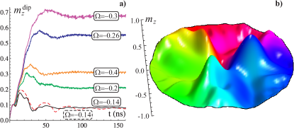
Figure 5: (Color online) Multidip structure formation under the influence of the field (16) with $\mu=-3$ and $b$=0.008. The data were obtained from SLASI simulations for a disk with radius $L=50a$, thickness $h=5a$, exchange length $\ell=a$, and damping coefficient $\eta=0.1$. a) Solid curves correspond to the simulations in the laboratory reference frame for the rotating magnetic field with different frequencies $\Omega$. The dashed curve corresponds to the simulations in the RRF with $\Omega^{\text{rot}}=\Omega$ under the influence of a static field. b) Out-of-plane spin distributions from simulations in the RRF with $\Omega^{\text{rot}}=0.3$ at the moment $\tau\approx 24$ (same color code as in Fig. 2).

First of all we performed SLASI simulations in the laboratory frame of reference. Here the spin–lattice simulations agree with our micromagnetic results. In particular, the resonance behavior of the multidip structure is well–pronounced in Fig. 5a) (solid curves), with a maximum dip amplitude about the frequency $\Omega=0.3$.

The total energy of the magnet in the continuum limit in the RRF (19) has two main differences in comparison with the laboratory reference frame. First of all, instead of the time dependent Zeeman energy (17), one has the influence of a constant field with the same intensity. Apart of this, there appears an additional rotation energy $\mathscr{E}^{\text{rot}}=\widetilde{\Omega}J_{z}$. For the discrete system one can perform a similar transformation, using the discrete Zeeman energy of the interaction with a constant field. The discrete analogue of the rotation energy is determined by the discrete version of the $J_{z}$ momentum (12). Results of numerical simulations in the rotating frame of reference are plotted by the dashed curve in Fig. 5a) for the rotational frequency $\Omega^{\text{rot}}=0.3$; they are in a good agreement with simulations in the laboratory reference frame for $\Omega=0.3$. Note that we presented on Fig. 5a) simulations in the RRF for small enough rotational frequencies. The reason is that $J_{z}$ is not a good characteristics of the discrete system: both exchange and dipolar interaction break the conservation of $J_{z}$, since there is no rotation invariance of the discrete system. Therefore simulations in the RRF works well when the contribution of the $J_{z}$ term in the discrete Hamiltonian is small enough, and the discreteness effects are small. This is valid for small enough frequencies of the rotations, see Fig. 5a), or for high frequencies but small enough times, see Fig. 5b).

IV Analytical description of the dip creation

In order to describe the problem analytically, we consider the problem in the RRF. As we have seen using SLASI simulations, the dip can be considered as a stationary state of the system in the RRF.

To gain some insight how the interaction with the magnetic field (which is static in the rotating frame) together with the rotation provides the multidip creation we use the Ansatz (14). In order to simplify the model we consider the dip formation on a background of a pure in–plane vortex with $\cos\theta^{\text{v}}$=0. This approximation is confirmed by our numerical simulations, as well as by a previous study. Kravchuk et al. (2009) The field pumps directly only the mode with azimuthal number $m=\mu$. This mode is coupled, first of all, to the mode with $m=-\mu,0,\pm 2\mu$. Thus we will consider modes with $m=0,\pm\mu,\pm 2\mu$. Taking into account only cubic nonlinear terms in the magnetic energy, one can use the Ansatz (14) to calculate the effective Lagrangian

$$\mathscr{L}_{\text{eff}}=-\sum_{m=0;\pm\mu;\pm 2\mu}\alpha_{m}^{\star}\dot{\beta}_{m}-\mathscr{E}_{\text{eff}}$$ (23)

and the effective dissipation function

$$\begin{split}\mathscr{F}^{\text{eff}}=\frac{\eta}{2}\sum_{m}\Bigl{[}&\mathcal{A}_{m}\dot{\alpha}_{m}\left(\dot{\alpha}_{m}^{\star}-\frac{2im\Omega}{\mu}\alpha_{m}^{\star}\right)\\ +&\mathcal{B}_{m}\dot{\beta}_{m}\left(\dot{\beta}_{m}^{\star}-\frac{2im\Omega}{\mu}\beta_{m}^{\star}\right)\Bigr{]},\end{split}$$ (24)

where $\mathcal{A}_{m}=\langle f_{m}^{2}\rangle$ and $\mathcal{B}_{m}=\langle g_{m}^{2}\rangle$.

The effective energy consists of several parts $\mathscr{E}_{\text{eff}}=\mathscr{E}_{\text{eff}}^{\text{osc}}+\mathscr{E}_{\text{eff}}^{\text{f}}+\mathscr{E}_{\text{eff}}^{\text{rot}}+\mathscr{E}_{\text{eff}}^{\text{int}}$, where

$$\mathscr{E}_{\text{eff}}^{\text{osc}}=\frac{1}{2}\sum_{m}\varOmega_{|m|}\left(|\alpha_{m}|^{2}+|\beta_{m}|^{2}\right)$$ (25)

describes the linear part of the modes oscillation, the energy of the interaction with the field $\mathscr{E}_{\text{eff}}^{\text{f}}$ is equal to $\widetilde{\mathscr{E}}^{\text{f}}$ in (20), the rotation energy

$$\mathscr{E}_{\text{eff}}^{\text{rot}}=-i\frac{\Omega}{\mu}\sum_{m}m\alpha_{m}\beta_{m}^{\star}$$ (26)

appears due to the transition into the noninertial frame of reference, and the energy of the nonlinear coupling between the modes has the form

$$\begin{split}\mathscr{E}_{\text{eff}}^{\text{int}}=i\sum_{m,n}m(k_{m,n}^{\alpha}\alpha_{m}\alpha_{n}+k_{m,n}^{\beta}\beta_{m}\beta_{n})\beta_{m+n}^{\star}.\end{split}$$ (27)

For the explicit form of the magnon frequencies $\varOmega_{m}$ and the nonlinearity coefficients $k_{i,j}^{\xi}$ see Appendix C.

Assuming that the nonlinear coefficients take approximately the same values $k_{i,j}^{\xi}\approx k$ one can obtain the equations of motion for the amplitudes $\alpha_{m}$, $\beta_{m}$ in the form

$$\begin{split}\dot{\alpha}_{m}=&\varOmega_{m}\beta_{m}+b_{e}(\delta_{m,\mu}+\delta_{m,-\mu})-i\Omega\frac{m}{\mu}\alpha_{m}\\ -&ik\sum_{m^{\prime}}{m^{\prime}}\alpha_{m^{\prime}}^{\star}\alpha_{{m^{\prime}}+m}+\eta\mathcal{B}_{m}\left(\dot{\beta}_{m}+i\frac{m}{\mu}\Omega\beta_{m}\right),\\ \dot{\beta}_{m}=&-\varOmega_{m}\alpha_{m}-i\Omega\frac{m}{\mu}\beta_{m}+ik\sum_{m^{\prime}}({m^{\prime}}+m)\alpha_{m^{\prime}}^{\star}\beta_{{m^{\prime}}+m}\\ -&\eta\mathcal{A}_{m}\left(\dot{\alpha}_{m}+i\frac{m}{\mu}\Omega\alpha_{m}\right).\end{split}$$ (28)

In the infinite set of equations (28) we restrict ourselves to the finite number of equations which do not contain any amplitudes $\alpha_{i},\beta_{i}$, with the exception of amplitudes with indices $i=0,\pm\mu,\pm 2\mu$. The obtained system was solved numerically for the case $\mu=3$ and different field amplitudes. The values of the corresponding eigenfrequencies $\varOmega_{0,\mu,2\mu}$ were chosen to be equal to the ones obtained from extra micromagnetic simulations of the magnon dynamics, these values are marked by dashed circles in Fig. 1. The frequencies $\varOmega_{0}$ and $\varOmega_{|\mu|}$ correspond to the lowest modes with radial number $n=0$ while $\varOmega_{|2\mu|}$ corresponds to the mode with $n=1$, because of two reasons: (i) according to the Fourier spectra in Fig. 2 and Fig. 3 the mode with this radial number dominates among modes with azimuthal number $m=2\mu$; (ii) as it will be shown later the second resonance $R_{2}$ (see Fig. 4,b) appears at the frequency $\varOmega_{2\mu}/2$ which corresponds to the mode with $n=1$ (see Fig.1). According to the mentioned spectra the amplitude of the dips in a multidip structure is determined mainly by the value $\alpha_{\mu}$, i.e. the amplitude of the out-of-plane component of the mode with $m=\mu$. The numerically obtained dependencies $|\alpha_{\mu}(t)|$ are shown in the Fig. 6a). These dependencies are in good agreement with the behavior of the dips depth, obtained using simulations, see Fig. 4a). Moreover, the steady-state value of $\alpha_{\mu}$ has the same properties as the steady-state dips depth $m_{z}^{\mathrm{dip}}$: (i) its frequency dependence has a resonance character, (ii) the resonance frequency is lower than the eigenfrequency, see Fig. 6a). Amplitude-frequency characteristics obtained numerically from model (28) (Fig. 6b-d) let us conclude that the phenomenon of an abrupt appearance of a dip (multidip) structure in a vortex state is a nonlinear resonance in a system of nonlinearly coupled modes with $m=0,\pm\mu,\pm 2\mu$. The corresponding resonance transition is shown as $R_{1}$ in Fig. 4b) and in Fig. 6b)-d).

In the no–damping and weakly nonlinear limit ($k\ll 1$) the stationary values $\bar{\alpha}_{m}$ and $\bar{\beta}_{m}$ can be represented approximately as follows:

$$\begin{split}\bar{\alpha}_{\mu}&=-\frac{ib_{e}\Omega}{\Omega^{2}-\varOmega_{\mu}^{2}},\qquad\bar{\beta}_{\mu}=i\bar{\alpha}_{\mu}\frac{\varOmega_{\mu}}{\Omega},\\ \bar{\alpha}_{0}&=-\frac{2k\mu\varOmega_{\mu}\left|\bar{\alpha}_{\mu}\right|^{2}}{\Omega\varOmega_{0}}=\frac{-2k\mu b_{e}^{2}\varOmega_{\mu}\Omega}{\varOmega_{0}\left(\Omega^{2}-\varOmega_{\mu}^{2}\right)^{2}},\quad\bar{\beta}_{0}=0,\\ \bar{\alpha}_{2\mu}&=\frac{k\mu\bar{\alpha}_{\mu}^{2}}{\Omega}\frac{2\Omega^{2}+\varOmega_{\mu}\varOmega_{2\mu}}{4\Omega^{2}-\varOmega_{2\mu}^{2}},\quad\bar{\beta}_{2\mu}=ik\mu\bar{\alpha}_{\mu}^{2}\frac{2\varOmega_{\mu}+\varOmega_{2\mu}}{4\Omega^{2}-\varOmega_{2\mu}^{2}}.\end{split}$$ (29)

According to the last two equations an additional resonance is expected for the frequency $\Omega=\varOmega_{2\mu}/2$. This resonance is observed in the simulation results (see Fig. 4, b) and it is well recognized in Fig. 6 b-e, is denoted as $R_{2}$.

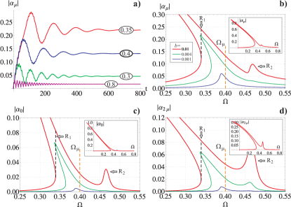
Figure 6: (Color online) The nonlinear resonance in system (28). Subfigure a) demonstrates time dependencies of the amplitude of the out-of-plane component of the mode with $m=\mu$. The shown dependencies were obtained numerically directly from (28) for different field frequencies $\Omega$ (the values are in the oval frames). The values of the other parameters were the following: $\mu=3$, $\varOmega_{\mu}=0.4$, $\varOmega_{0}=0.47$, $\varOmega_{2\mu}=0.92$, $b=0.01$, $\eta=0.02$, $k=0.1$, $\mathcal{A}_{i}=\mathcal{B}_{i}=1$. Amplitude-frequency characteristics for different modes are presented in the subfigures b)-d). The numerical values of the parameters are the same as in subfigure a). The thick (red) curve is build for the field amplitude $b=0.01$, thus it fully corresponds to the subfig. a). The small insets shows the mentioned curve in full scale.

V Conclusions

We have presented a detailed study of the dip structure generation, which always precedes the vortex polarity switching phenomenon. The physical reason for the dip creation is softening of a magnon mode and consequently a nonlinear resonance in the system of certain magnon modes with nonlinear coupling. The usually observed single-dip structure is a particular case of a multidip structure. The dynamics of the structure with $n$ dips can be strictly described as the dynamics of nonlinearly coupled modes with azimuthal numbers $m=0,\pm n,\pm 2n$. The multidip structure with an arbitrary number of dips (or vortex-antivortex pairs) can be obtained in a vortex-state nanodisk using a space- and time-varying magnetic field of the form (16). A scheme of a possible experimental setup for multidip structure generation is proposed in Appendix B.

Appendix A Dipolar interaction and the conservation of the total momentum

In this Appendix we consider a ferromagnetic system described by the classical Heisenberg isotropic exchange Hamiltonian

$$\mathcal{H}^{\text{ex}}=-\frac{J}{2}\sum_{\left(\bm{n},\bm{\delta}\right)}\bm{S}_{\bm{n}}\cdot\bm{S}_{\bm{n}+\bm{\delta}}$$ (30)

and the dipolar interaction $\mathcal{H}^{\text{dip}}$:

$$\mathcal{H}^{\text{dip}}=\frac{D}{2}\sum_{\begin{subarray}{c}\bm{n},\bm{n}^{\prime}\\ \bm{n}\neq\bm{n}^{\prime}\end{subarray}}\frac{\bm{S}_{\bm{n}}\cdot\bm{S}_{\bm{n}^{\prime}}-3\left(\bm{S}_{\bm{n}}\cdot\bm{e}_{\bm{n}\bm{n}^{\prime}}\right)\left(\bm{S}_{\bm{n}^{\prime}}\cdot\bm{e}_{\bm{n}\bm{n}^{\prime}}\right)}{|\bm{n}-\bm{n}^{\prime}|^{3}}.$$ (31)

Here $\bm{S}_{\bm{n}}\equiv\left(S^{x}_{\bm{n}},S^{y}_{\bm{n}},S^{z}_{\bm{n}}\right)$ is a classical spin vector with fixed length $S$ in units of action on the site $\bm{n}=(n_{x},n_{y},n_{z})$ of a three–dimensional cubic lattice with integers $n_{x}$, $n_{y}$, $n_{z}$, $J$ is the exchange integral, the parameter $D=\gamma^{2}/a^{3}$ is the strength of the long–range dipolar interaction, $\gamma=g|e|/(2mc)$ is the gyromagnetic ratio, $g$ is the Landé–factor, $a$ is the lattice constant; the vector $\bm{\delta}$ connects nearest neighbors, and $\bm{e}_{\bm{n}\bm{n}^{\prime}}\equiv\left(\bm{n}-\bm{n}^{\prime}\right)/\left|\bm{n}-\bm{n}^{\prime}\right|$ is a unit vector.

Our main approximation is that $\bm{S}_{\bm{n}}$ depends only on the $x$ and $y$ coordinates. Such a plane–parallel spin distribution is adequate for thin films with a constant thickness $h=N_{z}a$ and nanoparticles with small aspect ratio. Using the above mentioned approximation the dipolar Hamiltonian can be written as follows: Caputo et al. (2007)

$$\begin{split}&\mathcal{H}^{\text{dip}}=-\frac{D}{2}\sum_{\begin{subarray}{c}{\bm{\nu}},{\bm{\nu^{\prime}}}\end{subarray}}\Bigl{[}A_{{\bm{\nu}}{\bm{\nu^{\prime}}}}\left(\bm{S}_{{\bm{\nu}}}\cdot\bm{S}_{{\bm{\nu^{\prime}}}}-3S_{{\bm{\nu}}}^{z}S_{{\bm{\nu^{\prime}}}}^{z}\right)\\ &+B_{{\bm{\nu}}{\bm{\nu^{\prime}}}}\left(S_{{\bm{\nu}}}^{x}S_{{\bm{\nu^{\prime}}}}^{x}-S_{{\bm{\nu}}}^{y}S_{{\bm{\nu^{\prime}}}}^{y}\right)+C_{{\bm{\nu}}{\bm{\nu^{\prime}}}}\left(S_{{\bm{\nu}}}^{x}S_{{\bm{\nu^{\prime}}}}^{y}+S_{{\bm{\nu}}}^{y}S_{{\bm{\nu^{\prime}}}}^{x}\right)\Bigr{]}\!.\!\!\!\end{split}$$ (32)

Here the sum runs only over the 2D lattice. All the information about the original 3D structure of our system is in the coefficients $A_{{\bm{\nu}}{\bm{\nu^{\prime}}}}$, $B_{{\bm{\nu}}{\bm{\nu^{\prime}}}}$ and $C_{{\bm{\nu}}{\bm{\nu^{\prime}}}}$,

$$\begin{split}A_{{\bm{\nu}}{\bm{\nu^{\prime}}}}&=\frac{1}{2}\sum_{\begin{subarray}{c}{n^{\prime}}_{z},n_{z}\\ r_{\bm{n}\bm{n^{\prime}}}\neq 0\end{subarray}}\frac{r_{\bm{n}\bm{n^{\prime}}}^{2}-3z_{\bm{n}\bm{n^{\prime}}}^{2}}{r_{\bm{n}\bm{n^{\prime}}}^{5}},\\ B_{{\bm{\nu}}{\bm{\nu^{\prime}}}}&=\frac{3}{2}\sum_{\begin{subarray}{c}{n^{\prime}}_{z},n_{z}\\ r_{\bm{n}\bm{n^{\prime}}}\neq 0\end{subarray}}\frac{x_{\bm{n}\bm{n^{\prime}}}^{2}-y_{\bm{n}\bm{n^{\prime}}}^{2}}{r_{\bm{n}\bm{n^{\prime}}}^{5}},\\ C_{{\bm{\nu}}{\bm{\nu^{\prime}}}}&=3\sum_{\begin{subarray}{c}{n^{\prime}}_{z},n_{z}\\ r_{\bm{n}\bm{n^{\prime}}}\neq 0\end{subarray}}\frac{x_{\bm{n}\bm{n^{\prime}}}y_{\bm{n}\bm{n^{\prime}}}}{r_{\bm{n}\bm{n^{\prime}}}^{5}},\end{split}$$ (33)

where we used the notations: $x_{\bm{n}\bm{n^{\prime}}}=a(n_{x}-{n^{\prime}}_{x})$, $y_{\bm{n}\bm{n^{\prime}}}=a(n_{y}-{n^{\prime}}_{y})$, $z_{\bm{n}\bm{n^{\prime}}}=a(n_{z}-{n^{\prime}}_{z})$, $\rho_{{\bm{\nu}}{\bm{\nu^{\prime}}}}=\sqrt{x_{\bm{n}\bm{n^{\prime}}}^{2}+y_{\bm{n}\bm{n^{\prime}}}^{2}},\;r_{\bm{n}\bm{n^{\prime}}}=\sqrt{\rho_{{\bm{\nu}}{\bm{\nu^{\prime}}}}^{2}+z_{\bm{n}\bm{n^{\prime}}}^{2}}$.

The continuum description of the system is based on smoothing the lattice model, using the normalized magnetization $\bm{m}(\bm{r})=\left({g\mu_{B}}/{a^{3}M_{S}}\right)\sum_{\bm{n}}\bm{S}_{\bm{n}}\delta(\bm{r}-\bm{r}_{\bm{n}})$. Then the exchange energy $\mathscr{E}^{\text{ex}}$ (normalized by $4\pi M_{S}^{2}$), the continuum version of (30), takes the form (2). The normalized magnetostatic energy, which is the continuum version of (32), is

$$\begin{split}&\mathscr{E}^{\text{ms}}=-\frac{1}{16\pi}\int\mathrm{d}^{3}\bm{r}\int\mathrm{d}^{3}\bm{r^{\prime}}\frac{\mathcal{W}\left[\bm{m},\bm{m^{\prime}}\right]}{R^{5}},\\ &\mathcal{W}\left[\bm{m},\bm{m^{\prime}}\right]=\left(R^{2}-3|z-z^{\prime}|^{2}\right)\Bigl{[}\sin\theta\sin\theta^{\prime}\cos\left(\phi-\phi^{\prime}\right)\\ &-2\cos\theta\cos\theta^{\prime}\Bigr{]}+3\sin\theta\sin\theta^{\prime}\Bigl{[}\rho^{2}\cos\left(\phi+\phi^{\prime}-2\chi\right)\\ &+{\rho^{\prime}}^{2}\cos\left(\phi+\phi^{\prime}-2\chi^{\prime}\right)-2\rho\rho^{\prime}\cos\left(\phi+\phi^{\prime}-\chi-\chi^{\prime}\right)\Bigr{]},\\ &R\left(\bm{r},\bm{r^{\prime}}\right)=\sqrt{\rho^{2}+{\rho^{\prime}}^{2}-2\rho\rho^{\prime}\cos(\chi-\chi^{\prime})+(z-z^{\prime})^{2}}.\end{split}$$ (34)

The magnetostatic energy in the form (34) is invariant under to simultaneous rotations of $\phi$ and $\chi$ with the same constant angle $\varphi_{0}$, see Eq. (11).

The consequence of such an invariance is the conservation of the total momentum (12). Let us show explicitly that $J_{z}$ is conserved. The time derivative of the total momentum

$$\begin{split}\frac{\mathrm{d}J_{z}}{\mathrm{d}t}&=\int\!\mathrm{d}^{3}\bm{r}\partial_{\chi}\left(\frac{1-\cos\theta}{\sin\theta}\cdot\frac{\partial\mathscr{E}}{\partial\theta}\right)\\ &+\int\!\mathrm{d}^{3}\bm{r}\left(\cos\theta-1\right)\left[\partial_{\chi},\partial_{t}\right]\phi,\\ &+\int\!\mathrm{d}^{3}\bm{r}\left(\frac{\delta\mathscr{E}}{\delta\phi}-\frac{\delta\mathscr{E}}{\delta\phi}\partial_{\chi}\phi-\frac{\delta\mathscr{E}}{\delta\theta}\partial_{\chi}\theta\right)\end{split}$$ (35)

where we used an explicit form of Eqs. (6) in the case of absence of magnetic field and damping. The first term in (35) vanishes due to the cylindrical symmetry of the sample. The second term contains the commutator $\left[\partial_{\chi},\partial_{t}\right]\phi$; it can take nonvanishing values for the singular field distributions like 2D solitons and vortices with $\phi=q\chi+\text{const}$, which results in $[\partial_{x},\partial_{y}]\phi=2\pi q\delta(\bm{r})$.Papanicolaou and Tomaras (1991) Nevertheless this singularity does not influence the last term in (35) due to the vanishing factor $(\cos\theta-1)$ at the singularity point. This replacement $\cos\theta\to\cos\theta-1$ corresponds to the regularization of the Lagrangian Sheka (2006).

Let us discuss the last term in (35). Since an isotropic exchange interaction allows the conservation of $M_{z}$ and $L_{z}$ separately, we need to discuss here the influence of the magnetostatic interaction only. Using the explicit form (34), one can rewrite (35) as follows

$$\frac{\mathrm{d}J_{z}}{\mathrm{d}t}=\frac{1}{8\pi}\!\!\int\!\!\frac{\mathrm{d}^{3}\bm{r}\mathrm{d}^{3}\bm{r^{\prime}}}{R^{5}}\Biggl{[}\frac{\partial\mathcal{W}}{\partial\theta}\partial_{\chi}\theta+\frac{\partial\mathcal{W}}{\partial\phi}\left(\partial_{\chi}\phi-1\right)\Biggr{]}=\frac{I_{1}+I_{2}}{8\pi}.$$

Here the contribution $I_{1}$ takes the form:

$$I_{1}=\!\int\!\!\frac{\mathrm{d}^{3}\bm{r}\mathrm{d}^{3}\bm{r^{\prime}}}{R^{5}}\frac{\partial\mathcal{W}}{\partial\chi}\!=\!\int\!\!\mathrm{d}^{3}\bm{r}\mathrm{d}^{3}\bm{r^{\prime}}\Biggl{[}\!\frac{\partial}{\partial\chi}\!\!\left(\frac{\mathcal{W}}{R^{5}}\right)-\mathcal{W}\!\frac{\partial}{\partial\chi}\!\!\left(\frac{1}{R^{5}}\right)\Biggr{]}.$$

The first integral vanishes due to periodicity on $\chi$ and cylindrical symmetry. The derivative in the last term

$$\frac{\partial}{\partial\chi}\!\!\left(\frac{1}{R^{5}}\right)=-\frac{5\rho\rho^{\prime}}{R^{7}}\sin\left(\chi-\chi^{\prime}\right)$$

is asymmetric with respect to the replacement $\bm{r}\leftrightarrow\bm{r^{\prime}}$, hence this term vanishes after the integration, and $I_{1}=0$.

The integral $I_{2}=\int\mathrm{d}^{3}\bm{r}\mathrm{d}^{3}\bm{r^{\prime}}F[\bm{r},\bm{r^{\prime}}]$ has the asymmetrical kernel

$$\begin{split}F[\bm{r},\bm{r^{\prime}}]&=\sin\theta\sin\theta^{\prime}\Bigl{[}\left(R^{2}-3|z-z^{\prime}|^{2}\right)\sin\left(\phi-\phi^{\prime}\right)\\ &+{\rho^{\prime}}^{2}\sin\left(\phi+\phi^{\prime}-2\chi^{\prime}\right)-\rho^{2}\sin\left(\phi+\phi^{\prime}-\chi-\chi^{\prime}\right)\Bigr{]}\\ &=-F[\bm{r^{\prime}},\bm{r}],\end{split}$$

therefore, $I_{2}=0$.

Finally, one can state that the total momentum $J_{z}$ is conserved for a cylindrical sample under the action of magnetostatic interaction. One should note that the conservation of $J_{z}$ is known for the local model of the magnetostatic interaction $\mathscr{E}_{\text{loc}}^{\text{ms}}=\varkappa\int\!\mathrm{d}^{3}\bm{r}\left(\nabla\cdot\bm{m}\right)^{2}$. Papanicolaou and Tomaras (1991)

Appendix B Experimental possibility of a multidip structure creation

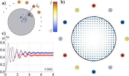
Figure 7: (Color online) Possible implementation of an experimental facility for pumping of a selected azimuthal magnon mode. Subfig. a) demonstrates the utility assembling. Subfig. b) shows the magnetic field (36) within the disk area. The number of the wires is $N=12$ and the phase shift of the currents is $\Delta\phi=\pi/2$ (corresponds to $m=3$, see text). Blue and red lines in subfig. c) illustrate dependencies $m_{z}^{\mathrm{dip}}(t)$ obtained using the field (16) with $\mu=-3$ (see Fig. 2 e) and the field (37) with $m=3$, respectively. In both cases the field amplitude was 15mT at the disk edge. $L=76$nm, $h=$20nm.

Let us consider a set of long conductive wires orientated perpendicular to the disk plane. Let all these wires be uniformly spaced along a circle which is concentric with the disk and has radius a $R>L$. The described configuration is shown in Fig. 7 a).

Let the $n$-th wire conduct the current $I_{n}=I\cos(\omega t+2\pi mn/N)$, where $N$ is the total number of the wires, $m$ is the azimuthal number of the mode we aim to excite and $\omega$ should be close to the corresponding eigenfrequency $\Omega_{m}$. The described set of wires produces a magnetic field of the form

$$\bm{B}(\bm{r},\chi)=\frac{1}{c}\sum\limits_{n=0}^{N-1}I_{n}\frac{[\bm{e}_{z}\times(\bm{r}-\bm{R}_{n})]}{(\bm{r}-\bm{R}_{n})^{2}},$$ (36)

where $\bm{R}_{n}=R[\cos(2\pi n/N),\,\sin(2\pi n/N),0]$ is the radius-vector of the $n$-th wire, $(r,\chi,z)$ are coordinates of a cylindrical frame of reference with $\bm{e}_{z}$ being oriented directly to the reader, and $c$ denotes the speed of light. For the case $N\gg m$ one can proceed from the sum in (36) to an integral. And for the case $L\ll R$ the obtained integral yields

$$B_{x}(\xi,\chi)=\frac{NI}{2Rc}\Bigl{\{}$$

$$\sin[\omega t-(m-1)\chi]\left[\xi^{|m-1|}-\xi^{|m|+1}\right]-$$

$$\sin[\omega t-(m+1)\chi]\left[\xi^{|m+1|}-\xi^{|m|+1}\right]\Bigr{\}},$$ (37a)

$$B_{y}(\xi,\chi)=-\frac{NI}{2Rc}\Bigl{\{}$$

$$\cos[\omega t-(m-1)\chi]\left[\xi^{|m-1|}-\xi^{|m|+1}\right]+$$

$$\cos[\omega t-(m+1)\chi]\left[\xi^{|m+1|}-\xi^{|m|+1}\right]\Bigr{\}},$$ (37b)

where $\xi=r/R\ll 1$. The field (37) corresponds to the field (16) with $\mu=-|m|$ and $\mathrm{sgn}(\omega)=\mathrm{sgn}(m)$, but contrary to (16) it is radially dependent. The radial dependence does not change the ability of the field (37) for the production of multidip structures. The radial dependent field results only in a small decreasing of the dips amplitude, see Fig.7 c). The accuracy of conformity of (37) with (36) strongly depends on $N$. Using the minimal number of the wires $N=2m$ one can excite the standing wave with azimuthal number $m$. To obtain the multidip structure one should take $2m<N\leq 4m$. It is senseless to take $N>4m$ because it does not improve the accuracy significantly. Satisfactory accuracy was achieved for $L/R<1/2$.

Appendix C Microscopic expressions for magnon frequencies and nonlinearity coefficients

Substitution of the Ansatz (14) into (2) and integration results in:

$$\begin{split}&\mathscr{E}_{ex}=\frac{1}{2}\frac{\ell^{2}}{h^{2}}\varepsilon^{2}\sum_{m}\Bigl{[}|\alpha_{m}|^{2}\left\langle f_{m}^{\prime 2}+(m^{2}-1)\frac{f_{m}^{2}}{\rho^{2}}\right\rangle\\ &+|\beta_{m}|^{2}\left\langle g_{m}^{\prime 2}+m^{2}\frac{g_{m}^{2}}{\rho^{2}}\right\rangle\Bigr{]}\\ &+\sqrt{2}i\frac{\ell^{2}}{h^{2}}\varepsilon^{2}\sum_{m,n}\alpha_{m}\alpha_{n}\beta_{m+n}^{\star}m\left\langle\frac{f_{m}f_{n}g_{m+n}}{\rho^{2}}\right\rangle+\mathcal{O}(\alpha^{4},\beta^{4}).\end{split}$$ (38)

Using that for a weakly excited in-plane vortex state $\varphi=\chi+\mathfrak{C}\frac{\pi}{2}+\tilde{\varphi}$, $m_{z}=\tilde{m}_{z}$ the divergence has the form

$$\nabla\cdot\bm{m}=-\frac{\mathfrak{C}}{\rho}\left[\rho\frac{\partial\tilde{\varphi}}{\partial\rho}+\tilde{m}_{z}\frac{\partial\tilde{m}_{z}}{\partial\chi}+\tilde{\varphi}\left(2+\frac{\partial\tilde{\varphi}}{\partial\chi}\right)\right]+\mathcal{O}(\tilde{m}_{z}^{3},\tilde{\varphi}^{3}),$$ (39)

one can perform a similar action to obtain the corresponding magnetostatic terms:

$$\begin{split}&\mathscr{E}_{ms}^{v}=\frac{\varepsilon}{2}\sum_{m}|\beta_{m}|^{2}\left\langle\gamma_{m}(\rho)\gamma_{m}(\rho^{\prime})\right\rangle_{m}^{\mathrm{ms(v)}}\\ &+\frac{i\varepsilon}{\sqrt{2}}\sum_{m,n}m\Biggl{[}\alpha_{n}\alpha_{m}\beta_{m+n}^{\star}\left\langle\gamma_{m+n}(\rho)\frac{f_{n}(\rho^{\prime})f_{m}(\rho^{\prime})}{\rho^{\prime}}\right\rangle_{m+n}^{\mathrm{ms(v)}}\\ &+\beta_{m}\beta_{n}\beta_{m+n}^{\star}\left\langle\gamma_{m+n}(\rho)\frac{g_{n}(\rho^{\prime})g_{m}(\rho^{\prime})}{\rho^{\prime}}\right\rangle_{m+n}^{\mathrm{ms(v)}}\Biggr{]}+\mathcal{O}(\alpha^{4},\beta^{4}),\end{split}$$ (40)

$$\mathscr{E}_{ms}^{s}=\frac{1}{2\varepsilon}\sum_{m}|\alpha_{m}|^{2}\left\langle f_{m}(\rho)f_{m}(\rho^{\prime})\right\rangle_{m}^{\mathrm{ms(s)}},$$ (41)

$$\begin{split}&\mathscr{E}_{ms}^{e}=-\varepsilon\sum_{m}|\beta_{m}|^{2}\left\langle\gamma_{m}(\rho)g_{m}(1)\right\rangle_{m}^{\mathrm{ms(e)}}\\ &-\frac{i\varepsilon}{\sqrt{2}}\sum_{m,n}m\Biggl{[}\alpha_{n}\alpha_{m}\beta_{m+n}^{\star}\left\langle\frac{f_{n}(\rho)f_{n}(\rho)g_{m+n}(1)}{\rho}\right\rangle_{m+n}^{\mathrm{ms(e)}}\\ &+\beta_{n}\beta_{m}\beta_{m+n}^{\star}\left\langle\frac{g_{n}(\rho)g_{m}(\rho)g_{m+n}(1)}{\rho}\right\rangle_{m+n}^{\mathrm{ms(e)}}\Biggr{]}+\mathcal{O}(\alpha^{4},\beta^{4}).\end{split}$$ (42)

The notation

$$\gamma_{m}(\rho)=\frac{\partial g_{m}(\rho)}{\partial\rho}+2\frac{g_{m}(\rho)}{\rho}$$ (43)

is used here and three different types of averaging are defined:

$$\begin{split}&\langle F(\rho,\rho^{\prime})\rangle_{k}^{\mathrm{ms(v)}}\equiv(-1)^{k}\int_{0}^{1}\mathrm{d}\rho\rho\int_{0}^{1}\mathrm{d}\rho^{\prime}\rho^{\prime}F(\rho,\rho^{\prime})\int_{0}^{\infty}\frac{e^{-\varepsilon x}-1+\varepsilon x}{\varepsilon^{2}x^{2}}J_{k}(\rho x)J_{k}(\rho^{\prime}x)\mathrm{d}x\\ &\langle F(\rho,\rho^{\prime})\rangle_{k}^{\mathrm{ms(s)}}\equiv(-1)^{k}\int_{0}^{1}\mathrm{d}\rho\rho\int_{0}^{1}\mathrm{d}\rho^{\prime}\rho^{\prime}F(\rho,\rho^{\prime})\int_{0}^{\infty}(1-e^{-\varepsilon x})J_{k}(\rho x)J_{k}(\rho^{\prime}x)\mathrm{d}x\\ &\langle F(\rho)\rangle_{k}^{\mathrm{ms(e)}}\equiv(-1)^{k}\int_{0}^{1}\mathrm{d}\rho\rho F(\rho)\int_{0}^{\infty}\frac{e^{-\varepsilon x}-1+\varepsilon x}{\varepsilon^{2}x^{2}}J_{k}(\rho x)J_{k}(x)\mathrm{d}x.\end{split}$$ (44)

Comparing (40)–(42) with (25) and (27) one can conclude that the eigenfrequencies read

$$\begin{split}\varOmega_{m}=&\frac{\ell^{2}}{h^{2}}\varepsilon^{2}\left\langle f_{m}^{\prime 2}+(m^{2}-1)\frac{f_{m}^{2}}{\rho^{2}}\right\rangle+\frac{1}{\varepsilon}\left\langle f_{m}(\rho)f_{m}(\rho^{\prime})\right\rangle_{m}^{\mathrm{ms(s)}}\\ =&\frac{\ell^{2}}{h^{2}}\varepsilon^{2}\left\langle g_{m}^{\prime 2}+m^{2}\frac{g_{m}^{2}}{\rho^{2}}\right\rangle+\varepsilon\left\langle\gamma_{m}(\rho)\gamma_{m}(\rho^{\prime})\right\rangle_{m}^{\mathrm{ms(v)}}-2\varepsilon\left\langle\gamma_{m}(\rho)g_{m}(1)\right\rangle_{m}^{\mathrm{ms(e)}},\end{split}$$ (45)

and the nonlinearity coefficients have form

$$\begin{split}k_{m,n}^{\alpha}=&\sqrt{2}\frac{\ell^{2}}{h^{2}}\varepsilon^{2}\left\langle\frac{f_{m}f_{n}g_{m+n}}{\rho^{2}}\right\rangle+\frac{\varepsilon}{\sqrt{2}}\left[\left\langle\gamma_{m+n}(\rho)\frac{f_{n}(\rho^{\prime})f_{m}(\rho^{\prime})}{\rho^{\prime}}\right\rangle_{m+n}^{\mathrm{ms(v)}}-\left\langle\frac{f_{n}(\rho)f_{n}(\rho)g_{m+n}(1)}{\rho}\right\rangle_{m+n}^{\mathrm{ms(e)}}\right],\\ k_{m,n}^{\beta}=&\frac{\varepsilon}{\sqrt{2}}\left[\left\langle\gamma_{m+n}(\rho)\frac{g_{n}(\rho^{\prime})g_{m}(\rho^{\prime})}{\rho^{\prime}}\right\rangle_{m+n}^{\mathrm{ms(v)}}-\left\langle\frac{g_{n}(\rho)g_{n}(\rho)g_{m+n}(1)}{\rho}\right\rangle_{m+n}^{\mathrm{ms(e)}}\right].\end{split}$$ (46)

It is interesting to emphasize the following properties of the energy expansions: (i) The linear part of the magnetostatic energy proportional to $|\beta|^{2}$ is produced by the volume charges, while the part proportional to $|\alpha|^{2}$ is produced by surface charges; (ii) The nonlinear terms of the magnetostatic energy appear due to the volume charges only; (iii) The exchange produces nonlinear terms of the form $\alpha\alpha\beta$. The same is true for magnetostatics, but additional terms in the form $\beta\beta\beta$ also appear.

References

- Wachowiak et al. (2002) A. Wachowiak, J. Wiebe, M. Bode, O. Pietzsch, M. Morgenstern, and R. Wiesendanger, Science 298, 577 (2002), eprint http://www.sciencemag.org/cgi/reprint/298/5593/577.pdf, URL http://www.sciencemag.org/cgi/content/abstract/298/5593/577.
- Chou et al. (2007) K. W. Chou, A. Puzic, H. Stoll, D. Dolgos, G. Schutz, B. V. Waeyenberge, A. Vansteenkiste, T. Tyliszczak, G. Woltersdorf, and C. H. Back, Appl. Phys. Lett. 90, 202505 (pages 3) (2007), URL http://link.aip.org/link/?APL/90/202505/1.
- Hubert and Schäfer (1998) A. Hubert and R. Schäfer, Magnetic domains: the analysis of magnetic microstructures (Springer–Verlag, Berlin, 1998).
- Skomski (2003) R. Skomski, J. Phys. C 15, R841 (2003), URL http://dx.doi.org/10.1088/0953-8984/15/20/202.
- Cowburn (2002) R. P. Cowburn, J. Magn. Magn. Mater. 242-245, 505 (2002), URL http://dx.doi.org/10.1016/S0304-8853(01)01086-1.
- Van Waeyenberge et al. (2006) B. Van Waeyenberge, A. Puzic, H. Stoll, K. W. Chou, T. Tyliszczak, R. Hertel, M. Fähnle, H. Bruckl, K. Rott, G. Reiss, et al., Nature 444, 461 (2006), ISSN 0028-0836, URL http://dx.doi.org/10.1038/nature05240.
- Xiao et al. (2006) Q. F. Xiao, J. Rudge, B. C. Choi, Y. K. Hong, and G. Donohoe, Appl. Phys. Lett. 89, 262507 (pages 3) (2006), URL http://link.aip.org/link/?APL/89/262507/1.
- Hertel et al. (2007) R. Hertel, S. Gliga, M. Fähnle, and C. M. Schneider, Phys. Rev. Lett. 98, 117201 (pages 4) (2007), URL http://link.aps.org/abstract/PRL/v98/e117201.
- Lee et al. (2007) K.-S. Lee, K. Y. Guslienko, J.-Y. Lee, and S.-K. Kim, Phys. Rev. B 76, 174410 (pages 5) (2007), URL http://link.aps.org/abstract/PRB/v76/e174410.
- Yamada et al. (2007) K. Yamada, S. Kasai, Y. Nakatani, K. Kobayashi, H. Kohno, A. Thiaville, and T. Ono, Nat Mater 6, 270 (2007), ISSN 1476-1122, URL http://dx.doi.org/10.1038/nmat1867.
- Kravchuk et al. (2007) V. P. Kravchuk, D. D. Sheka, Y. Gaididei, and F. G. Mertens, J. Appl. Phys. 102, 043908 (2007), URL http://link.aip.org/link/?JAP/102/043908/1.
- Sheka et al. (2007) D. D. Sheka, Y. Gaididei, and F. G. Mertens, Appl. Phys. Lett. 91, 082509 (2007), URL http://link.aip.org/link/?APL/91/082509/1.
- Liu et al. (2007) Y. Liu, H. He, and Z. Zhang, Appl. Phys. Lett. 91, 242501 (pages 3) (2007), URL http://link.aip.org/link/?APL/91/242501/1.
- Vansteenkiste et al. (2009) A. Vansteenkiste, K. W. Chou, M. Weigand, M. Curcic, V. Sackmann, H. Stoll, T. Tyliszczak, G. Woltersdorf, C. H. Back, G. Schutz, et al., Nat Phys 5, 332 (2009), ISSN 1745-2473, URL http://dx.doi.org/10.1038/nphys1231.
- Weigand et al. (2009) M. Weigand, B. V. Waeyenberge, A. Vansteenkiste, M. Curcic, V. Sackmann, H. Stoll, T. Tyliszczak, K. Kaznatcheev, D. Bertwistle, G. Woltersdorf, et al., Phys. Rev. Lett. 102, 077201 (pages 4) (2009), URL http://link.aps.org/abstract/PRL/v102/e077201.
- Gaididei et al. (2008) Y. B. Gaididei, V. P. Kravchuk, D. D. Sheka, and F. G. Mertens, Low Temperature Physics 34, 528 (2008), URL http://link.aip.org/link/?LTP/34/528/1.
- Gaididei et al. (2010) Y. Gaididei, V. P. Kravchuk, and D. D. Sheka, International Journal of Quantum Chemistry 110, 83 (2010), URL http://dx.doi.org/10.1002/qua.22253.
- Lee et al. (2008) K.-S. Lee, S.-K. Kim, Y.-S. Yu, Y.-S. Choi, K. Y. Guslienko, H. Jung, and P. Fischer, Phys. Rev. Lett. 101, 267206 (pages 4) (2008), URL http://link.aps.org/abstract/PRL/v101/e267206.
- Vansteenkiste et al. (2008) A. Vansteenkiste, K. W. Chou, M. Weigand, M. Curcic, V. Sackmann, H. Stoll, T. Tyliszczak, G. Woltersdorf, C. H. Back, G. Schütz, et al., X-ray imaging of the dynamic magnetic vortex core deformation (2008), eprint arXiv:0811.1348, URL http://arxiv.org/abs/0811.1348.
- Kravchuk et al. (2009) V. P. Kravchuk, Y. Gaididei, and D. D. Sheka, Phys. Rev. B 80, 100405 (pages 4) (2009), URL http://link.aps.org/abstract/PRB/v80/e100405.
- Papanicolaou and Tomaras (1991) N. Papanicolaou and T. N. Tomaras, Nuclear Physics B 360, 425 (1991), URL http://www.sciencedirect.com/science/article/B6TVC-470F3HY-36%/2/69a5e1a128fb5b7ef2ee0c512c3d78fc.
- Mertens and Bishop (2000) F. G. Mertens and A. R. Bishop, in Nonlinear Science at the Dawn of the 21th Century, edited by P. L. Christiansen, M. P. Soerensen, and A. C. Scott (Springer–Verlag, Berlin, 2000), pp. 137–170.
- Caputo et al. (2007) J.-G. Caputo, Y. Gaididei, V. P. Kravchuk, F. G. Mertens, and D. D. Sheka, Phys. Rev. B 76, 174428 (pages 13) (2007), URL http://link.aps.org/abstract/PRB/v76/e174428.
- Sheka (2006) D. D. Sheka, Journal of Physics A: Mathematical and General 39, 15477 (2006), URL http://stacks.iop.org/0305-4470/39/15477.