A Deeper Look at Leo IV: Star Formation History and Extended Structure

Abstract

We present MMT/Megacam imaging of the Leo IV dwarf galaxy in order to investigate its structure and star formation history, and to search for signs of association with the recently discovered Leo V satellite. Based on parameterized fits, we find that Leo IV is round, with $\epsilon<0.23$ (at the 68% confidence limit) and a half-light radius of $r_{h}\simeq 130$ pc. Additionally, we perform a thorough search for extended structures in the plane of the sky and along the line of sight. We derive our surface brightness detection limit by implanting fake structures into our catalog with stellar populations identical to that of Leo IV. We show that we are sensitive to stream-like structures with surface brightness $\mu_{r}\lesssim 29.6$ mag arcsec^-2, and at this limit, we find no stellar bridge between Leo IV (out to a radius of $\sim$0.5 kpc) and the recently discovered, nearby satellite Leo V. Using the color magnitude fitting package StarFISH, we determine that Leo IV is consistent with a single age ($\sim$14 Gyr), single metallicity ($[Fe/H]\sim-2.3$) stellar population, although we can not rule out a significant spread in these value. We derive a luminosity of $M_{V}=-5.5\pm 0.3$. Studying both the spatial distribution and frequency of Leo IV’s ’blue plume’ stars reveals evidence for a young ($\sim$2 Gyr) stellar population which makes up $\sim$2% of its stellar mass. This sprinkling of star formation, only detectable in this deep study, highlights the need for further imaging of the new Milky Way satellites along with theoretical work on the expected, detailed properties of these possible ’reionization fossils’.

1. Introduction

Since 2005, 14 satellite companions to the Milky Way have been discovered (see Willman (2010) and references therein). Despite the fact that many of these objects are less luminous than a typical globular cluster ($-1.5<M_{V}<-8.6$), these 14 objects have a range of properties that encompass the most extreme of any galaxies, including: the highest inferred dark matter content (e.g. Simon & Geha 2007; Geha et al. 2009), the lowest [Fe/H] content (Kirby et al. 2008), unusually elliptical morphologies (e.g. Hercules; Coleman et al. 2007; Sand et al. 2009), and in some cases evidence for severe tidal disturbance (e.g. Ursa Major II; Zucker et al. 2006; Munoz et al. 2009). The varied properties of these lowest luminosity galaxies are valuable probes for understanding the physics of dark matter and galaxy formation on the smallest scales.

Of the newly discovered Milky Way (MW) satellites, Leo IV ($M_{V}=-5.5$, $r_{h}\sim 130$ pc) is among the least studied, despite several signs that it is an intriguing object. Leo IV appears to be dominated by an old and metal-pool stellar population (de Jong et al. 2008b). However it also has an apparently complex color magnitude diagram (CMD), with a ’thick’ red giant branch, possibly caused by either multiple stellar populations and/or depth along the line of sight (Belokurov et al. 2007). Leo IV also may have a very extended stellar distribution, despite its apparently round ($\epsilon=0.22^{+0.18}_{-0.22}$) and compact ($r_{h}=2.5^{+0.5}_{-0.7}$ arcmin; Martin et al. 2008b) morphology. A search for variable stars was recently performed by Moretti et al. (2009), who used the average magnitude of three RR Lyrae stars to find a distance modulus of $(m-M)=20.94\pm 0.07$ mag, corresponding to $154\pm 5$ kpc. Interestingly, one of the three RR Lyrae variables lies at a projected radius of $\sim$10 arcmin, roughly three times the half light radius, leading to the suggestion that Leo IV may actually possess a ’deformed morphology’.

Based on Keck/DEIMOS spectroscopy of 18 member stars, Leo IV has one of the smallest velocity dispersions of any of the new MW satellites, with $\sigma=3.3\pm 1.7$ km/s (Simon & Geha 2007). A metallicity study of 12 of these spectra (Kirby et al. 2008) showed Leo IV to be extremely metal poor, with $\langle[Fe/H]\rangle=-2.58$ with an intrinsic scatter of $\sigma_{[Fe/H]}=0.75$ – the highest dispersion among the new dwarfs.

Recently, the MW satellite Leo V ($M_{V}\sim-4.3\pm 0.3$) has been discovered, separated by only $\sim$2.8 degrees on the sky and $\sim$40 km/s from Leo IV (Belokurov et al. 2008). With a Leo V distance of $\sim$180 kpc, this close separation in phase space led Belokurov et al. (2008) to suggest that the Leo IV/Leo V system may be physically associated. This argument was bolstered by Walker et al. (2009), who spectroscopically identified two possible Leo V members 13 arcminutes from the satellite’s center (Leo V’s $r_{h}$ is $\sim$0.8 arcminutes) along the line connecting Leo IV and Leo V, suggesting that Leo V is losing mass. A recent analysis by de Jong et al. (2010) of two 1 square degree fields situated between Leo IV and Leo V shows tentative evidence for a stellar ’bridge’ between the two systems with a surface brightness of $\sim$32 mag arcsec^-2.

Motivated by all the above, we obtained deep photometry of Leo IV with Megacam on the MMT. In this paper, we use these data to present a detailed analysis of both the structure and SFH of Leo IV. We also search for any signs of disturbance in Leo IV which may hint at a past interaction with the recently discovered, nearby Leo V. In § 2 we describe the observations, data reduction and photometry. We also present our final catalog of Leo IV stars. In § 3 we derive the basic structural properties of Leo IV, and search for signs of extended structure. We quantitatively assess the stellar population of Leo IV in § 4 using both CMD-fitting software and an analysis of its blue plume population. We discuss and conclude in § 5.

2. Observations and Data Reduction

We observed Leo IV on April 21 2009 (UT) with Megacam (McLeod et al. 2000) on the MMT. MMT/Megacam has 36 CCDs, each with $2048\times 4608$ pixels at 0$\farcs$08/pixel (which were binned $2\times 2$), for a total field-of-view (FOV) of $\sim$24’$\times$24’. We obtained 5 250s dithered exposures in $g$ and in $r$ in clear conditions with 0$\farcs$9 seeing. We reduced the data using the Megacam pipeline developed at the Harvard-Smithsonian Center for Astrophysics by M. Conroy, J. Roll and B. McLeod, which is based in part on M. Ashby’s Megacam Reduction Guide. The pipeline includes standard image reduction tasks such as bias subtraction, flatfielding and cosmic ray removal. Precise astrometric solutions for each science exposure were derived using the Sloan Digital Sky Survey Data Release 6 (SDSS-DR6 Adelman-McCarthy et al. 2006) and the constituent images were then resampled onto a common grid (using the lanczos3 interpolation function) and combined with SWarp using the weighted average.

Stellar photometry was determined on the final image stack using a nearly identical methodology as Sand et al. (2009) with the command line version of the DAOPHOTII/Allstar package (Stetson 1994). We allowed for a quadratically varying PSF across the field when determining our model PSF and ran Allstar in two passes – once on the final stacked image and then again on the image with the first round’s stars subtracted, in order to recover fainter sources. We culled our Allstar catalogs of outliers in $\chi^{2}$ versus magnitude, magnitude error versus magnitude and sharpness versus magnitude space to remove objects that were not point sources. In general, these cuts varied as a function of magnitude. We positionally matched our $g$ and $r$ band source catalogs with a maximum match radius of 0$\farcs$5, only keeping those point sources detected in both bands in our final catalog.

Instrumental magnitudes are put onto a standard photometric system using stars in common with SDSS-DR6. We used all SDSS stars within the field of view with $17.5<r<21.5$ and $-0.25<g-r<1.5$ to perform the photometric calibration and simultaneously fit for a zeropoint and a linear color term in $g-r$. The linear color term slope was 0.11 in ($r-r_{MMT}$) versus $(g-r)$ and 0.086 in ($g-g_{MMT}$) versus $(g-r)$, consistent with that found in the MMT study of Bootes II by Walsh et al. (2008). Slight residual zeropoint gradients across the field of view were fit to a quadratic function and corrected for (see also Saha et al. 2010), resulting in a final overall scatter about the best-fit zeropoint of $\delta g\sim$0.05 and $\delta r\sim$0.05 mag.

To calculate our photometric errors and completeness as a function of magnitude and color, we performed a series of artificial star tests using a technique nearly identical to that of Sand et al. (2009). Briefly, artificial stars were placed into our Leo IV images on a regular grid with spacing between ten and twenty times the image full width at half maximum with the DAOPHOT routine ADDSTAR. In all, ten iterations were performed on our Leo IV field for a total of $\sim$300000 implanted artificial stars. The $r$ magnitude for a given artificial star was drawn randomly from 18 to 29 mag, with an exponentially increasing probability toward fainter magnitudes. The $g-r$ color is then randomly assigned over the range -0.5 to 1.5 with equal probability. These artificial star frames were then run through the same photometry pipeline as the unaltered science frames, applying the same $\chi^{2}$, sharpness and magnitude-error cuts. For reference, we are 50% (90%) complete in $g$ at $\sim$25.3 (23.6) mag and in $r$ at 24.8 (23.3) mag. When necessary, such as for calculating the SFH of Leo IV in § 4, the completeness as a function of both magnitude and color is taken into account.

2.1. The Color Magnitude Diagram and Final Leo IV Catalog

We present the CMD of Leo IV in Figure 1. Plotted in the left panel are all stars within the half-light radius (as determined in § 3.1), while in the right panel we present a Hess diagram of the same field with a scaled background subtracted using stars located outside a radius of 12 arcminutes.

In both panels we highlight the possible stellar populations of Leo IV. In the right panel we plot three theoretical isochrones from Girardi et al. (2004). The solid and dashed lines are old 14 Gyr isochrones with [Fe/H] of -2.3 and -1.7, respectively. We adjust these isochrones to have $m-M$=20.94, as found in the RR Lyrae study of Leo IV by Moretti et al. (2009), which fit the ridgeline well. With the dotted line, we also plot a 1.6 Gyr isochrone with [Fe/H]=-1.3. This isochrone agrees relatively well with the ’blue plume’ stars which are evident in Leo IV’s CMD.

We mark several regions in the left panel of Figure 1 for quantitative study in later sections. The solid box denotes the blue horizontal branch (BHB) stars, which are clearly defined in our CMD. The dashed and dotted regions are two different selection regions for blue plume stars. The dashed is the total blue plume population, although much of this region may be plagued by foreground stars or unresolved galaxies. We thus will also utilize the stars within the dotted box as a relatively contamination-free tracer of the blue plume star population in later sections. An open question is whether or not the blue plume stars are young stars, as is plausible based on the CMD, or are blue stragglers. We quantitatively assess the blue plume population in § 4.2.

Given that the CMD of Leo IV is visually in excellent agreement with the distance measurement of Moretti et al. (2009), and the possible presence of multiple stellar populations, we do not attempt a CMD-fitting method for measuring the distance to Leo IV (e.g., Sand et al. 2009), and will adopt $(m-M)=20.94$ throughout this work. We will vary this quantity when necessary to determine how sensitive our results are to this assumption.

We present our full Leo IV catalog in Table 1, which includes our $g$ and $r$ band magnitudes (uncorrected for extinction) with their uncertainty, along with the Galactic extinction values derived for each star (Schlegel et al. 1998). We also note whether the star was taken from the SDSS catalog rather than our MMT data, as was done for objects near the saturation limit of our Megacam data. Unless stated otherwise, all magnitudes reported in the remainder of this paper will be extinction corrected.

3. Leo IV Structural Properties

We split our analysis of the structural properties of Leo IV into two components. First, we fit parameterized models to the surface density profile of Leo IV. Following this, we search for signs of extended structure in Leo IV, especially in light of its proximity to Leo V.

3.1. Parameterized Fit

It is common to fit the surface density profile of both globular clusters and dSphs to King (King 1966), Plummer (Plummer 1911), and exponential profiles. This is an important task both to facilitate comparisons with other observational studies and for understanding the MW satellites as a population (e.g., Martin et al. 2008b). To do this, we use the CMD selection region shown in Figure 2 for isolating likely Leo IV members. This CMD selection box was determined by first taking a M92 ridgeline at $(m-M)$=20.94, the distance to Leo IV found by Moretti et al. (2009), and placing two bordering selection boundaries a minimum of 0.1 mag on either side in the $g-r$ color direction. These selection regions are increased to match the typical $g-r$ color uncertainty at a given $r$ magnitude (as determined with our artificial star tests) when that number exceeds 0.1 mag. A magnitude limit of $r$=24.8 mag was applied to correspond to our 50% completeness limit. At the present we focus on Leo IV ridge line stars, but we discuss the spatial properties of the blue plume and horizontal branch stars in § 4.2.

We fit the three parameterized density profiles to the stellar distribution of Leo IV:

$$\Sigma_{King}(r)=\Sigma_{0,K}\left(\left(1+\frac{r^{2}}{r_{c}^{2}}\right)^{-\frac{1}{2}}-\left(1+\frac{r_{t}^{2}}{r_{c}^{2}}\right)^{-\frac{1}{2}}\right)^{2}$$ (1)

$$\Sigma_{Plummer}(r)=\Sigma_{0,P}\left(1+\frac{r^{2}}{r_{P}^{2}}\right)^{-{2}}$$ (2)

$$\Sigma_{exp}(r)=\Sigma_{0,E}\exp\left(-\frac{r}{\alpha}\right)$$ (3)

where $r_{P}$ and $\alpha$ are the scale lengths for the Plummer and exponential profiles and $r_{c}$ and $r_{t}$ are the King core and tidal radii, respectively. For the Plummer profile, $r_{P}$ equals the half-light radius $r_{h}$, while for the exponential profile $r_{h}\approx 1.668\alpha$. We simultaneously fit a background surface density, $\Sigma_{b}$, while fitting the Plummer and exponential profiles. For the King profile, there is a degeneracy between the tidal radius and the background surface density. We thus fix the background value to the average of that found for the Plummer and exponential profiles for our King profile fits (e.g. Walsh et al. 2008).

We use a maximum likelihood (ML) technique for constraining structural parameters similar to that of Martin et al. (2008b), which we have refined in Sand et al. (2009), and further refined in the current work. We point the reader to those works for further details concerning the expression of the likelihood function. Including the central position, $\alpha_{0}$ and $\delta_{0}$, position angle ($\theta$), and ellipticity ($\epsilon$) both the exponential and Plummer profiles have the same free parameters – ($\alpha_{0}$,$\delta_{0}$,$\theta$,$\epsilon$,$r_{half}$,$\Sigma_{b}$), while the King profile free parameters are ($\alpha_{0}$,$\delta_{0}$,$\theta$,$\epsilon$,$r_{c}$,$r_{t}$). Uncertainties on structural parameters are determined through 1000 bootstrap resamples, from which a standard deviation is calculated. We have tested the robustness of our algorithm for dwarf galaxies with roughly the same number of stars as Leo IV in an Appendix, and will use these tests to inform our results in what follows.

Our results are presented in Table 2. We show our best fit stellar profiles in Figure A Deeper Look at Leo IV: Star Formation History and Extended Structure. Although the plotted stellar profiles are not fit to the plotted binned data points, they do show excellent agreement. We note that the apparent slight overdensity at $R\sim$8 arcmin above the derived parameterized fits does not correspond to any single feature, as can be seen from the smoothed map of Leo IV that we present in § 3.2 and Figure 3, but is likely just the result of several fluctuations at roughly the same radius. Interestingly, Leo IV appears to be particularly round, at least according to the parameterized model fit to the data. In fact, our ML-derived ellipticity is consistent with zero (see also the Appendix), allowing us to only place an upper limit of $\epsilon\lesssim 0.23$ (at the 68% confidence limit). Given this low ellipticity, we can not place any meaningful constraints on the position angle of Leo IV, as both the tests in the Appendix indicate and the bootstrap resamples of our Leo IV data reaffirm. On a separate note, the tidal radius for the King profile fit, with a value of $r_{t}=18.55^{\prime}$, is larger than the Megacam FOV. Thus, this value should be taken with caution.

It is useful to compare our parameterized fit results with similar work in the literature. Using the original SDSS data, Martin et al. (2008b) fit Leo IV with an exponential profile using a ML technique similar to the one utilized in the current work, and found results within 1-$\sigma$ of those presented here. More recently, de Jong et al. (2010) used deeper data from the 3.5 m Calar Alto telescope around both Leo IV and Leo V, again applying a ML algorithm to measure their structure. In this case, the authors find $r_{h}=4.6^{+0.8}_{-0.7}$ and a well measured ellipticity of $\epsilon=0.49\pm 0.11$, both statistically inconsistent with the results presented in the current work. As commented on by de Jong et al. (2010), this is likely because of the different stellar populations probed – while the present work uses mostly main sequence and subgiant stars to determine the structure of Leo IV, de Jong et al. (2010) use mostly brighter stars and objects on the blue horizontal branch. Also, Leo IV lies on the edge of one of their pointings, which could have biased their results. Resolution of this discrepancy will require additional measurements.

3.2. Extended Structure Search

We now search for signs of tidal disturbance and other anomalies – which would not be picked up by our parameterized fits in § 3.1 – based on the morphology of Leo IV’s isodensity contours. We do this with an eye towards determining if there is a current physical connection between Leo IV and Leo V.

Our basic approach is similar to that of Sand et al. (2009). We include stars within the same CMD selection box used for our parameterized fits (Figure 2), placed those stars in $10^{\prime\prime}\times 10^{\prime\prime}$ bins and spatially smoothed these pixels with three different Gaussians of $\sigma$=0.5,1.0 and 1.5 arcminutes. The background level of stars in the CMD selection box, and its variance, was determined via the MMM routine in IDL. To avoid the bulk of Leo IV, these statistics were determined in two boxes of size $20^{\prime}\times 3^{\prime}$ situated 9.5 arcminutes North and South of Leo IV. We found that our smoothed maps were unaffected if only one of these boxes was used, or if we varied their sizes. We present our smoothed maps in Figure 3, with the contours representing regions that are 3, 4, 5, 6, 7, 10 and 15 standard deviations above the background. We focus on the $\sigma$=0.5 arcminute map, since it contains the most detail without loss of potential Leo IV features. The $\sigma$=1.0 arcminute smoothing scale will be useful in § 3.2.1, as we explore our sensitivity to stellar streams.

Outside of the main body of Leo IV, there appears to be only a handful of compact, 3, 4 and 5 $\sigma$ overdensities. How significant are these overdensities, given the binning, smoothing and number of pixels that went into the making of Figure 3? To gauge their significance, we take our input photometric catalog, randomize the star positions and remake our smoothed maps (with the 0.5 arcmin Gaussian) for several realizations (Figure 4). While some of these maps have several 3 and 4 $\sigma$ overdensities, while others have fewer, we find that the distribution of pixel values maintains a Poisson distribution. We thus conclude that the majority of features outside the main body of Leo IV in Figure 3 are likely just noise – with the possible exception of the 5-$\sigma$ overdensities at positions $(\sim-6^{\prime},\sim 12^{\prime})$ and $(\sim-8^{\prime},\sim-10^{\prime})$ with respect to Leo IV. Background-subtracted Hess diagrams of these two regions were made from our Leo IV catalog, but they do not yield CMDs that are consistent with Leo IV’s stellar population (see § 3.2.1). Thus, our observations yield no strong evidence for substructure in the vicinity of Leo IV.

The main body of Leo IV itself has some interesting features. There is a hint of an elongation or disturbance in the core of Leo IV, along with two ’tendrils’ – one directed to the West and the other to the Southwest. Again, due to the small number of stars in Leo IV, these irregularities may be an effect of small number statistics. To evaluate the significance of the morphology in Figure 3, we follow the path of Walsh et al. (2008) and their evaluation of morphological irregularities in Bootes II. We bootstrap resample the Leo IV stars and replot our smoothed maps. The results of nine such resamples can be seen in Figure 5. While we cannot rule out that the tendrils seen in our Leo IV map are genuine, they are not ubiquitous features in our resampled maps, and so we cannot with confidence claim they are real features.

We finally point out that there appears to be no sign of interaction or disturbance in the direction of Leo V, which we indicate in the middle panel of Figure 3. A Hess diagram of all stars farther than 5 arcminutes from the center of Leo IV, and within 1.5 arcminutes of the line that connects Leo IV and Leo V, yields a differenced CMD that is consistent with noise (after proper background subtraction). Any such disturbance would have to be below our detection threshold, which we determine in the next section. Finally we point out that these smoothed maps are sensitive to structures at the distance of both Leo IV and Leo V ($\sim$180 kpc; Belokurov et al. 2009) given that we are predominantly probing the CMD at magnitudes brighter than the subgiant branch.

3.2.1 Inserting Artificial Remnants

In order to assess our surface brightness limit, and our sensitivity to structures of different sizes and morphologies, we insert fake ’nuggets’ and ’streams’ into our Leo IV catalog with stellar populations drawn from one consistent with that of Leo IV. As in Sand et al. (2009), we use the testpop program within the CMD-fitting package, StarFISH, to generate our artificial ’Leo IV’ CMDs and then remake our smoothed maps. By varying the number of stars (and, by extension, the surface brightness) in these structures, we can then assess whether our adopted search method for extended structure would have recovered them, and if so, what the resulting CMD would look like. This method of ’observing’ and then examining these artificial remnants is more informative than traditional methods of simply quoting a ’$3-\sigma$’ surface brightness limit, even if the result is a relatively ambiguous detection limit. For details of the procedure, we refer the reader to Sand et al. (2009), and to our presentation of Leo IV’s SFH in § 4.

We inject both ’nuggets’ – Leo IV-like stellar populations with an exponential profile having $r_{half}=1.0$ arcmin – and ’streams’ – with a Gaussian density profile in the right ascension direction with $\sigma$=1.5 arcmin and a uniform distribution in the declination direction over the Northern half of the field – into our final Leo IV photometric catalog. In Figures 6 and 7, we illustrate some results from our tests, along with their properties in Table 3.

We show an example of a 35 star ’nugget’ near what we believe is our detection threshold in Figure 6. While this nugget has a peak detection at 6.4-$\sigma$, it is not particularly different in morphology or significance than the other random peaks in our Leo IV field. This, however, changes when the resulting Hess diagram is examined, showing several stars along the red giant branch – something that is not apparent in the true overdensities in our field. Taking this as our rough detection limit for compact remnants of Leo IV, we are sensitive to objects with a central surface brightness of $\mu_{0,r}=27.9$ and $\mu_{0,g}=28.3$.

Turning towards our artificial ’streams’, both the 200 and 300 star streams are easily detectable in our smoothed maps (where we have used a 1 arcminute smoothing scale to better pick out the thick streams – Figure 7). Further, the resulting Hess CMDs show a considerable red giant and BHB presence, and the beginnings of the main sequence for the 300 star case. The analogous 100 star stream is not convincingly detected. We thus suggest that we are reliably sensitive to streams with central surface brightness $\mu_{r}\sim 29.6$ and $\mu_{g}\sim 29.8$ (as measured along the center of the stream) with a geometry and morphology roughly similar to that simulated.

The recent work of de Jong et al. (2010) have presented tentative evidence for a stream connecting Leo IV and Leo V with a surface brightness of $\sim$32 mag arcsec^-2. Unfortunately, despite our much deeper data, we are unable to probe down to such faint surface brightness limits due to the relatively small area of our single pointing.

3.3. Structure along the line of sight

Because previous authors have suggested that the ’thick’ red giant branch in Leo IV may be due to elongation along the line of sight, it is worth searching for signs of such elongation in the width of the BHB (e.g., Klessen et al. 2003). To do this, we have created a BHB star fiducial using data collected by J. Strader from SDSS encompassing 41 horizontal branch stars from M3 and M13, corrected for extinction and their relative distances. Using these stars, a third-order polynomial was fit with the IDL routine robust_poly_fit, and we used this polynomial to define our BHB fiducial.

For simplicity, we assume that all stars in our Megacam field within the solid box in Figure 1 are BHB stars belonging to Leo IV. Placing the BHB fiducial at our assumed distance to Leo IV, $(m-M)=20.94$, leads to a visually excellent match. However, since we are interested in the scatter about this fiducial to put constraints on the width of Leo IV, rather than the absolute distance to it, we adjust the fiducial BHB sequence so that the average $r$ magnitude deviation of the Leo IV BHB stars against the fiducial is $\sim$0.0 (this adjustment was 0.06 mag, affirming the distance measurement of Moretti et al. (2009)). The resulting root mean square deviation of the Leo IV BHB stars about the fiducial is $\sim$0.2 mag, which corresponds to a deviation of $\sim$15 kpc at the distance of Leo IV. While this limit is comparable to the quoted difference in distance between Leo IV and Leo V (Belokurov et al. 2008), it is also roughly the measurement limit achievable using the spread in BHB mags as a measure of line-of-sight depth. First, there are known RR Lyrae variables among the BHB stars in Leo IV (Moretti et al. 2009), which we have observed at a random phase. Second, for a spread in metallicity of $\sigma_{[Fe/H]}=0.75$ in Leo IV (Kirby et al. 2008), one would expect a natural spread in BHB star magnitudes of $\sim$0.2 mag (Sandage & Cacciari 1990; Olszewski et al. 1996). We therefore conclude that our data, while consistent with no elongation along the line of sight, can not put strong constraints on the depth of Leo IV.

4. Stellar population

There is spectroscopic evidence that Leo IV has a large metallicity spread, and according to Kirby et al. (2008) it has the largest metallicity spread seen among the new dwarfs ($\langle[Fe/H]\rangle$=$-$2.58 with a spread of $\sigma_{[Fe/H]}$=0.75). Additionally, Belokurov et al. (2007) have hinted that Leo IV has a ’thick’ red giant branch, indicating a spread in metallicity, and this appears to be the case (at least superficially) in the CMD presented in the current work (Figure 1). Also intriguing is the population of blue plume stars pointed out in Figure 1 and § 2.1. In this section, we first perform a CMD-fitting analysis of the stellar population of Leo IV with StarFISH, and then go on to look at the blue plume population in detail. We end the section by combining the structural properties found in § 3.1 with the stellar population determined in the current section to calculate the total absolute magnitude of Leo IV.

4.1. Star Formation History via CMD-fitting

Here we apply the CMD-fitting package StarFISH (Harris & Zaritsky 2001) to our Leo IV photometry within the half light radius to determine its SFH and metallicity evolution. As discussed in previous works, StarFISH uses theoretical isochrones (we use those of Girardi et al. 2004, although any may be used) to construct artificial CMDs with different combinations of distance, age, and metallicity. Once convolved with the observed photometric errors and completeness (using the artificial star tests of § 2), these theoretical CMDs are converted into realistic model CMDs which can be directly compared to the data on a pixel-to-pixel basis, after binning each into Hess diagrams. We use the Poisson statistic of Dolphin (2002) as our fit statistic. The best fitting linear combination of model CMDs is determined through a modification of the standard AMOEBA algorithm (Press et al. 1988; Harris & Zaritsky 2001). Several steps are taken to determine the uncertainties in StarFISH fits, which are discussed in detail in previous work – see Harris & Zaritsky (2009); de Jong et al. (2008a).

Our StarFISH analysis is similar to that of Sand et al. (2009). We include isochrones with [Fe/H]=-2.3,-1.7 and -1.3 and ages between $\sim$10 Myr and $\sim$15 Gyr. Age bins of width $\Delta$log(t)=0.4 dex were adopted, except for the two oldest age bins centered at $\sim$10 Gyr and $\sim$14 Gyr, where the binning was $\Delta$log(t)=0.3 dex. A ’background/foreground’ CMD, created by taking all stars outside an elliptical radius of 12 arcminutes (with ellipticity of $\epsilon$=0.05, as in our best-fitting exponential profile, see Table 2), was simultaneously fit along with our input stellar populations in order to correct for contamination by unresolved galaxies and foregound stars in our Leo IV CMD.

Stars with magnitudes $18.0<r<24.75$ (corresponding roughly to our 50% completeness limit) and $-0.50<g-r<1.15$ were fit. After some experimentation, we used a Hess diagram bin size of 0.15 mag in magnitude and 0.15 mag in color. We assume a binary fraction of 0.5 and a Salpeter initial mass function. Because we correct our stellar catalog for Galactic extinction with the dust maps of Schlegel et al. (1998), we do not allow the mean extinction of our model CMDs to vary. As in the rest of this work, we chose to fix the distance modulus in the code to $(m-M)$=20.94 mag, although our results are robust with respect to this assumption, as we discuss below.

We show the best-fit StarFISH solution in Figure A Deeper Look at Leo IV: Star Formation History and Extended Structure, along with a comparison of the best model CMD with that of Leo IV in Figure 8. Leo IV is consistent with a single stellar population with an age of $\sim$14 Gyr and a [Fe/H]=-2.3, although the error bars and upper limits indicate that there is latitude for both a small, young stellar population and a mix of metallicities at older ages. Thus, despite the visual impression of a ’thick’ giant branch, our analysis does not require a metallicity spread to match the oberved CMD. Thorough spectroscopy of all stars in the red giant region will be required to determine Leo IV membership and to properly quantify the metallicity spread. This result is robust to small changes in the distance modulus. If we alter the input distance modulus from $(m-M)$=20.94 to $(m-M)$=20.84, than a larger fraction of the best-fitting SFH comes from the [Fe/H]=-1.3 bin, although the [Fe/H]=-2.3 bin still dominates. Likewise, a distance modulus of $(m-M)$=21.04 yields an old, [Fe/H]=-2.3 stellar population with even less from the [Fe/H]=-1.7 and -1.3 bins.

The model and observed CMDs match remarkably well (Figure 8) given that there are known mismatches between the theoretical isochrones and empirical, single population CMDs (e.g., Girardi et al. 2004). Also, the available models do not span the metallicity range that is apparent in the new MW dwarfs; Kirby et al. (2008) found $\langle[Fe/H]\rangle=-2.58$ with an intrinsic scatter of $\sigma_{[Fe/H]}=0.75$ in Leo IV, while the Girardi isochrone set reaches down to [Fe/H]=-2.3. There is a slight mismatch in the BHB between model and data, with the best-fitting model CMD having a BHB which is $\sim$0.1-0.2 mag brighter than that observed (this is a factor of $\sim$2 larger than the small BHB magnitude correction we made in § 3.3). This could be due to a slight error in our assumed distance modulus or a true stellar population that is even more metal poor than the most metal-poor model in the Girardi isochrone set, which we know to be the case from Kirby et al. (2008). Nonetheless, our basic finding that Leo IV is predominantly old ($\sim$14 Gyr) and metal poor is unaffected.

4.2. Evidence for Young Stars

It is well known that dwarf spheroidals harbor a population of blue stragglers – a hot, blue extension of objects which lie along the normal main sequence (e.g., Mateo et al. 1995). Because the densities in dwarfs do not reach that necessary to produce collisional binaries (as they can in the cores of globular clusters), it is likely that they are primordial binary systems, coeval with the bulk of stars in the dwarf. Unfortunately, their position along the main sequence makes it difficult to disentangle blue straggler stars from young main sequence stars in the MW’s dwarf spheroidals, which has been a continuous source of ambiguity (e.g., Mateo et al. 1995; Mapelli et al. 2007, 2009, among many others). It is very difficult to exclude the possibility that some of the blue plume stars in any given dwarf are actually young main sequence objects.

We now articulate two arguments in support of the hypothesis that at least some of the stars in the blue plume of Leo IV are young. First, the blue plume stars appear to be segregated within the body of Leo IV. We plot the position of the ’high probability’ blue plume stars with low background/foreground contamination, as identified within the dotted box in Figure 1, onto our smoothed map of Leo IV (Figure A Deeper Look at Leo IV: Star Formation History and Extended Structure). All of the selected high-probability blue plume stars within the body of Leo IV are on one side. If Leo IV is assumed to be spherically symmetric, the chances of all seven being on the same half of the galaxy are $\sim(1/2^{7})$ or less than 1 percent. This segregation would be difficult to explain if all of these objects were blue stragglers, which would presumably have the same distribution as the galaxy as a whole. We understand that this a posteriori argument is insufficient on its own, but it should be considered in the context of the high normalized blue plume fraction, which we now discuss.

Our second argument in favor of a young population of stars in Leo IV stems from the high blue plume frequency normalized by the BHB star counts, following the work of Momany et al. (2007). Briefly, Momany et al. (2007) sought to explore the ambiguity between young main sequence stars and genuine blue straggler stars in a sample of MW dwarf galaxies by calculating the number of total blue plume objects with respect to a reference stellar population – the BHB. The basic result of their work, whose data was kindly provided by Y. Momany, was that those dwarf spheroidals that do not have a true, young stellar component have a blue plume fraction that follows a relatively well defined $M_{V}$ vs log($N_{BP}/N_{BHB}$) anti-correlation, where the blue plume consists of only blue straggler stars (Figure A Deeper Look at Leo IV: Star Formation History and Extended Structure). The physical origin of this anti-correlation is unclear (see, however, Davies et al. 2004, for a plausible explanation for the anti-correlation in globular clusters), although it is seen in both open clusters (de Marchi et al. 2006) and globular clusters (Piotto et al. 2004). Carina, the one dwarf galaxy in their sample which does have a known, recent bout of star formation ($\sim$1-3 Gyr; Hurley-Keller et al. 1998; Monelli et al. 2003), was shown to have an excess of blue plume stars with respect to the aforementioned relation (shown as a lower limit in Figure A Deeper Look at Leo IV: Star Formation History and Extended Structure, due to difficulties in accounting for blue stragglers associated with the older and fainter main sequence turn-off in that system), pointing to the fact that Carina’s blue plume was populated with young main sequence stars in addition to a standard blue straggler population. More recently, Martin et al. (2008a) also found a high blue plume frequency in Canes Venatici I, which we also show in Figure A Deeper Look at Leo IV: Star Formation History and Extended Structure. Martin et al. (2008a) used the combination of spatial segregation and blue plume frequency to argue that Canes Venatici I harbors a young stellar component.

We take the ratio of blue plume to BHB stars as identified in Figure 1 by the dashed and solid regions, respectively, utilizing those stars within the half light radius of Leo IV and making background and completness corrections. We calculate a blue plume frequency of log($N_{BP}/N_{BHB}$)=$0.56\pm 0.13$ for Leo IV and plot this ratio along with those of the MW dwarf spheroidals just discussed in Figure A Deeper Look at Leo IV: Star Formation History and Extended Structure. As can be seen, Leo IV lies off the standard $M_{V}$ vs log($N_{BP}/N_{BHB}$) anti-correlation just as Canes Venatici I and Carina do. Leo IV lies $2-\sigma$ away from the linear relation fit by Momany et al. (2007) for the non-star forming dwarfs.

Taken together, the segregation of blue plume stars along with the high blue plume to BHB fraction points to at least some of the stars being young main sequence objects. We know that at least one of these blue plume stars is a blue straggler, due to the discovery of one SX Phoenicis variable in Leo IV (Moretti et al. 2009). This is only the third of the new dwarf spheroidals (excluding Leo T, which appears to be a transition object) that harbor a young stellar population – the others being the previously discussed Canes Venatici I (Martin et al. 2008a) and Ursa Major II (de Jong et al. 2008b). We note that our evidence for young stars is similar to that presented for Canes Venatici I, for which it was also found that the blue plume population is segregated and blue straggler frequency is high (Martin et al. 2008a). We measure the luminosity of the young stars in § 4.3 and discuss the implications of Leo IV’s young stellar component in § 5.

4.3. Absolute Magnitude

As pointed out by Martin et al. (2008b), measuring the total magnitudes of the new MW satellites is difficult due to the small number of stars at detectable levels. We account for this ’CMD shot noise’ by mimicking our measurement of the total magnitude of Hercules (Sand et al. 2009), which borrowed heavily from the original Martin et al. (2008b) analysis.

We take the best SFH solution presented in § 4.1, and create a well-populated CMD (of $\sim$200000 stars) incorporating our photometric completeness and uncertainties, using the repop program within the StarFISH software suite. We drew one thousand random realizations of the Leo IV CMD with an identical number of stars as we found for our exponential profile fit, and determined the ’observed’ magnitude of each realization above our 90% completeness limit. We then accounted for those stars below our 90% completeness level by using luminosity function corrections derived from Girardi et al. (2004), using an isochrone with a 15 Gyr age and [Fe/H]=-2.3. We take the median value of our one thousand random realizations as our measure of the absolute magnitude and its standard deviation as our uncertainty (Table 2). To convert from $M_{r}$ magnitudes to $M_{V}$ magnitudes we use $V-r=0.16$ (Walsh et al. 2008).

We find $M_{V}=-5.5\pm 0.3$ and a central surface brightness, assuming our exponential profile fit, of $\mu_{0,V}=27.2\pm 0.3$. Both our total absolute magnitude and central surface brightness measurement agrees to within $1-\sigma$ with the measurement of Martin et al. (2008b), which used only SDSS data.

We use a similar technique for determining the approximate luminosity of Leo IV’s young stellar population only. We draw an equivalent number stars from our well-populated StarFISH CMD as in Leo IV within our high probability blue plume box (see Figure 1 and § 4.2), and corrected for the luminosity of stars outside this region using a luminosity function derived from an isochrone with an age of 1.6 Gyr and [Fe/H]=-1.3 (Girardi et al. 2004). We again draw 1000 random realizations to determine our uncertainties. We find that the young stellar population has $M_{V}=-2.1\pm 0.5$, or roughly $\sim$5% of the satellite’s total luminosity or $\sim$2% of its stellar mass. This magnitude and the resulting fraction of the young stellar populations luminosity should be taken with caution given our assumptions and the small number of stars involved.

5. Discussion & Conclusions

In this work we have presented deep imaging of the Leo IV MW satellite with Megacam on the MMT and study this galaxy’s structure and SFH. In particular, we assess reports in the literature concerning both its stellar population and its possible association with the nearby satellite, Leo V.

Leo IV’s SFH is dominated by an old ($>12$ Gyr), metal poor ($[Fe/H]\lesssim-2.0$) stellar population, although we uncover evidence for a young sprinkling of star formation 1-2 Gyrs ago. Our best-fit StarFISH results indicate that a single metal poor population dominates, although the data is also compatible with a spread in metallicities. The old population is consistent with the emerging picture that the faintest MW satellites are ’reionization fossils’ (e.g.  Ricotti & Gnedin 2005; Gnedin & Kravtsov 2006), who formed their stars before reionization and then lost most of their baryons due to photoevaporation. The apparent sprinkling of young stars begs the question of what has enabled Leo IV to continue forming stars at a low level. There is no sign of HI in Leo IV, with an upper limit of 609 $M_{\odot}$ (Grcevich & Putman 2009), although we note that this limit is still a factor of $\sim$2 larger than the stellar mass associated with the young stellar population studied in § 4.2.

One possible mechanism for late gas accretion, and subsequent star formation, among the faint MW satellites was recently discussed by Ricotti (2009) to help explain the complex SFH and gas content of Leo T (de Jong et al. 2008a; Ryan-Weber et al. 2008). In this scenario, the smallest halos stop accreting gas after reionization as expected, but as their temperature decreases and dark matter concentration increases with decreasing redshift they are again able to accrete gas from the intergalactic medium at late times, assuming they themselves are not accreted by their parent halo until $z\lesssim 1-2$. This can lead to a bimodality in the SFH of the satellite, with both a $>12$ Gyr population and one that is $<10$ Gyr, as we see in Leo IV. One stringent requirement of this model is that the satellite can not have been accreted by its host halo until $z\lesssim 1-2$ (and thus not exposed to tidal stirring and ram pressure stripping until late times, allowing the satellite to retain its newly accreted gas). Future proper motion studies will be able to test if Leo IV is compatible with this late gas accretion model. Another prediction of this model is the possible existence of gas-rich minihaloes that never formed stars, but could serve as fuel for star formation if they encountered one of the luminous dwarfs. More detailed study of this late gas accretion mechanism will be necessary to understand the possible diversity of SFHs in the faint MW satellites.

Additionally, we note that if the apparent segregation of young stars in Leo IV is real, then it is not an isolated case among the MW satellites. As has been mentioned in § 4.2, Martin et al. (2008a) noted that Canes Venatici I has a compact star forming region clearly offset from the galaxy as a whole, with an age of 1-2 Gyrs, similar to Leo IV. Additionally, Fornax has several compact clumps and shells that house young stellar populations roughly $\sim$1.4 Gyrs old (Coleman et al. 2004, 2005; Olszewski et al. 2006). It has been suggested that these could have been the result of a collision between Fornax and a low-mass halo, which was possibly gas-rich. Peñarrubia et al. (2009) investigated the disruption of star clusters in triaxial, dwarf-sized halos and found that segregated structures can persist depending on the orbital properties of the cluster, providing yet another viable mechanism. More work is needed to distinguish between all of the above scenarios and to properly model the emerging diversity of SFHs among the new, faint MW satellites.

Structurally, Leo IV appears to be very round, with $\epsilon\lesssim 0.23$ (at the 68% confidence limit) and a half light radius ($\sim 130$ pc) which is typical of the new MW satellites. An exhaustive search for signs of extended structure in the plane of the sky has ruled out any associated streams with surface brightnesses of $\mu_{r}\lesssim 29.6$. The extent of Leo IV along the line of sight is less than $\sim$15 kpc, a limit that will be difficult to improve upon given the inherent limitations of using the spread in BHB magnitudes to measure depth. We find no evidence for structural anomalies or tidal disruption in Leo IV. We do not have the combination of image depth and area necessary to confirm the stellar bridge, with a surface brightness of 32 mag arcsec^-2, recently reported in between Leo IV and Leo V (de Jong et al. 2010). Indeed, Leo V is almost certainly disrupting, as discussed by Walker et al. (2009), due to the presence of two member stars $\sim$13 arcminutes ($>13r_{h}$) from Leo V’s center along the line connecting the putative Leo IV/Leo V system. The nature of Leo V is still very ambiguous, with the kinematic data being consistent with it being dark matter free – suggesting that perhaps Leo V is an evaporating star cluster (Walker et al. 2009). It is thus critical to obtain yet deeper data on these two systems and the region separating them to uncover their true nature.

The probable detection of a small population of young stars illustrates once again that it is crucial to obtain deep and wide field follow up for all of the newly detected MW satellites. Every new object has a surprise or two in store upon closer inspection.

6. Acknowledgements

We are grateful to the referee, Nicolas Martin, for his constructive report. Many thanks to Maureen Conroy, Nathalie Martimbeau, Brian McLeod and the whole Megacam team for the timely help in reducing our Leo IV data. DJS is grateful to Jay Strader for his excellent scientific advice, and for providing his co-calibrated M3 & M13 blue horizontal branch sequence. We are grateful to Evan Kirby, Josh Simon and Marla Geha for providing their kinematic and metallicity data on Leo IV. Yazan Momany kindly provided his blue plume frequency data. DJS is grateful to Matthew Walker and Nelson Caldwell for providing a careful reading of the paper, along with useful comments. EO was partially supported by NSF grant AST-0807498. DZ acknowledges support from NASA LTSA award NNG05GE82G and NSF grant AST-0307492.

7. Appendix

In this Appendix, we determine how well the maximum likelihood technique presented in § 3.1 can measure the structural parameters of a dwarf with a comparable number of stars as Leo IV. We create mock models of Leo IV-like systems having an exponential profile with $r_{h}$=3.0 arcmin and 400 stars in the input catalog (all on a footprint with the same area as our MMT pointing), while systematically varying the ellipticity and position angle. A uniform background of 4.5 stars per square arcminute is randomly scattered across the field to mimic the actual observations. We utilize the same algorithm as in § 3.1, with 1000 bootstrap resamples to determine our uncertainties.

We can recover the ellipticity of our mock dwarf galaxies remarkably well, as can be seen in Figure A Deeper Look at Leo IV: Star Formation History and Extended Structure. Here we show our results on the recovered ellipticity as a function of input model ellipticity, between $\epsilon_{input}=$0.05 and 0.85. The data points are the median ellipticity found for the one thousand bootstrap resamples for each model, and the error bars encompass 68% of the resamples around that median. Note that for models with an input ellipticity of $\epsilon\lesssim 0.25$ it is difficult for our algorithm to converge on the correct ellipticity value. In this regime, we present the measured ellipticity as an upper limit (see § 3.1). In this case, we systematically overpredict the ellipticity with large error bars, and thus only quote upper limits. Larger values of the ellipticity are well measured.

We also do a good job of measuring the position angle (as long as the ellipticity is high enough) and the half light radius of our mock Leo IV-like systems, which we illustrate in a series of examples in Figure 9. From the figure, one can see the gradual improvement in the measurement of the position angle as one goes from an ellipticity of 0.1 to 0.35, while the half light radius remains relatively well measured throughout. The slight systematic offset seen in the bottom left panel of Figure 9 can be explained due to the difficulty in recovering the true ellipticity for $\epsilon_{input}\lesssim 0.25$ systems. If one slightly overestimates the true input ellipticity of the data, this leads to a slight overestimation of the half-light radius, a degeneracy that can be seen in Figure 9 of Martin et al. (2008b). The take away message is that one must treat any ’measurement’ of the position angle with extreme caution for ellipticity values of $\epsilon\lesssim 0.25$ as we do in § 3.1.

In the future, we intend to present a more extensive series of tests of our maximum likelihood code in order to understand how star number and imaging field of view have on the estimation of structural parameters for the new MW satellites.

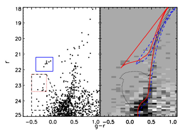
Figure 1.— Left – The CMD of Leo IV within $r_{h}$=2.85 arcmin. We note several regions marking off particular stellar populations. The dash-lined region encloses the total blue plume population, although any given star may be a foreground contaminant or unresolved galaxy. The inset dotted box is our high probability blue plume box, with relatively little galactic contamination. Finally, we consider those stellar objects within the solid-lined region to be BHB stars. We plot the spatial distribution of the high probability blue plume stars and the BHBs in Figure A Deeper Look at Leo IV: Star Formation History and Extended Structure. Right – A background subtracted Hess diagram of the same, central half light radius region of Leo IV. Overplotted are several theoretical isochrones from Girardi et al. (2004). The solid and dashed ridgelines are of a 14 Gyr stellar population with [Fe/H]=-2.3, -1.7, respectively. The dotted line is a $\sim$1.6 Gyr isochrone with [Fe/H]=-1.3, and roughly matches the overdensity of blue plume stars that are evident.

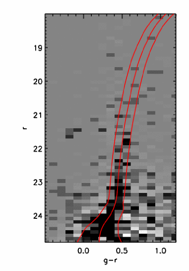
Figure 2.— An illustration of the CMD selection region used for performing our parameterized structural analysis of Leo IV. The figure is a background-subtracted Hess diagram of the central 2.5 arcminutes of Leo IV and the central, red fiducial ridge line is that of M92 transformed to a distance modulus of $(m-M)=20.94$. The two bordering ridge lines bound the selection region and are a minimum of 0.1 magnitudes in the color direction away from the M92 ridge line. The selection region expands to the size of the typical $g-r$ color uncertainty as a function of $r$ mag when this exceeds 0.1 mag, as determined via our artificial star tests. The selected region is an excellent match to the apparent ridgeline of Leo IV, as can be seen in the figure.

Stellar profile of Leo IV. The data points are the binned star counts for all stars within the CMD selection box shown in Figure 2. The plotted lines show the best fit one-dimensional exponential, Plummer and King profiles. The dotted line shows the background surface density determined for our exponential profile fit. Note that in deriving these best fits, we are not fitting to the binned data, but directly to the stellar distribution.

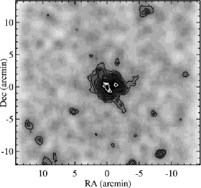
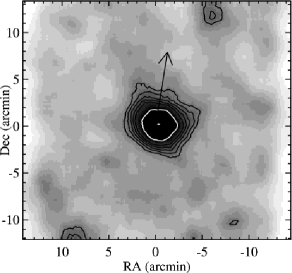
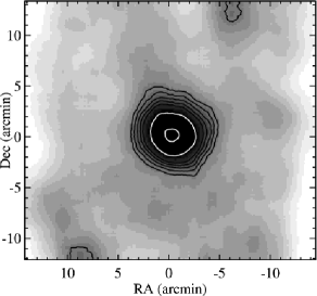
Figure 3.— Smoothed contour plots of Leo IV, showing the 3, 4, 5, 6, 7, 10 and 15 $\sigma$ levels. The left panel has been smoothed by 0.5 arcmin, the middle panel by 1.0 arcmin, and the right panel by 1.5 arcmin. The arrow in the middle panel indicates the direction to Leo V. Note that there is no apparent structure along this direction. The 3 $\sigma$ contour in our 0.5 arcminute smoothed map corresponds roughly to a surface brightness of $\sim$30.0 mag per arcsecond².

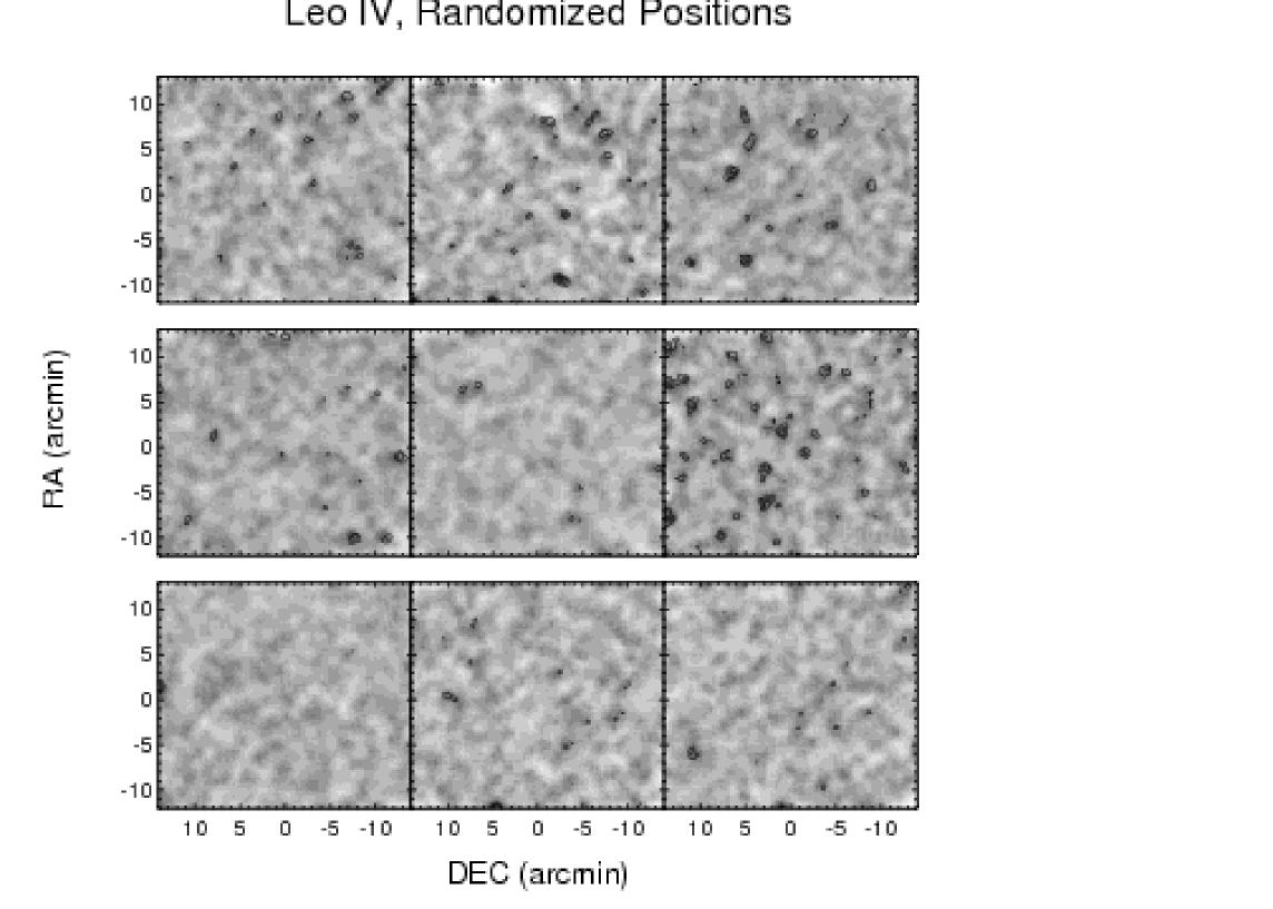
Figure 4.— Smoothed contour plots of nine random realizations of Leo IV stars, where we have reassigned star positions randomly across the Megacam field of view. The contours show the 3, 4 and 5 $\sigma$ levels. The plots show that compact 3 and 4 $\sigma$ overdensities are relatively common.

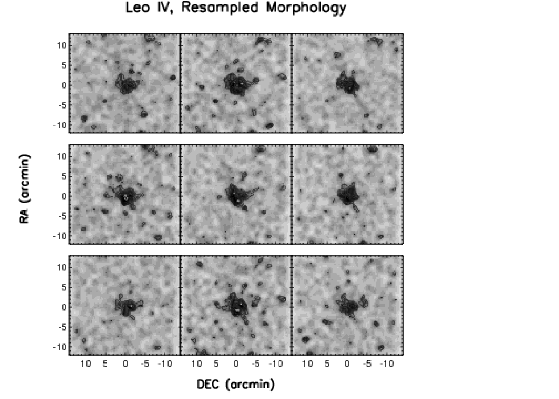
Figure 5.— Smoothed contour plots of 9 random bootstrap resamples of Leo IV stars (with the 0.5 arcminute Gaussian), showing how morphology can vary with each iteration. The contours show the 3, 4, 5, 6, 7, 10 and 15 $\sigma$ levels. While in some iterations the ’tendrils’ seen in Figure 3 are still visible, they are not a ubiquitous feature. Future, deeper imaging is necessary to confirm their reality.

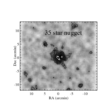
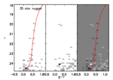
Figure 6.— An illustration of our technique for implanting fake Leo IV ’nuggets’ into our field, using an artificial stellar population drawn from that determined in our star formation history analysis (§ 4.1) and our artificial star tests (§ 2). Left: We show our smoothed map of Leo IV after implanting a 35 star ’nugget’ at $(+5^{\prime},+5^{\prime})$ with respect to the center of Leo IV, distributed as an exponential profile with a half-light radius of 1 arcminute (see Table 3). This nugget results in a $\sim$6.4-$\sigma$ overdensity at that position. Right: A Hess diagram of the 35 star nugget, along with a M92 isochrone shifted to $(m-M)=20.94$. This Hess diagram shows the raw star counts in the circular aperture shown in the left panel of this figure, along with an equal area background region, and the difference between the two. Note that the residual CMD shows several stars that would be identified with Leo IV’s red giant branch, which would allow us to say with confidence that such an overdensity is likely associated with Leo IV.

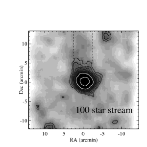
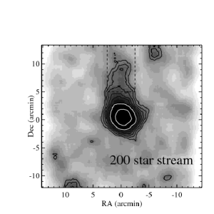
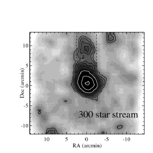
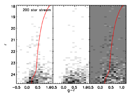
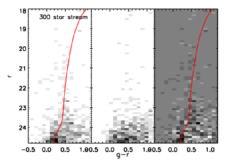
Figure 7.— An illustration of our technique for implanting fake Leo IV ’streams’ into our field. Top: We show our smoothed maps (using a 1 arcminute Gaussian) of Leo IV after implanting streams with different numbers of stars (see Table 3). Note that the 200 and 300 star streams are clearly detected. Bottom: The resulting Hess diagrams for our 200 and 300 star scenarios. Note that each has many obvious red giant and BHB members, while the 300 star stream has the beginnings of the main sequence. We show the region we used for extracting the ’stream’ photometry in our maps in the top row of this figure.

SFH solution from the StarFISH fit. With the data in hand, Leo IV is consistent with a single, old ($\sim$14 Gyr) stellar population with [Fe/H]$\sim$-2.3 – although there is some weak evidence for a spread in metallicity in this old stellar component. We also can not rule out a small, young population of stars with our StarFISH analysis. Error bars with no accompanying histogram are upper limits.

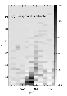
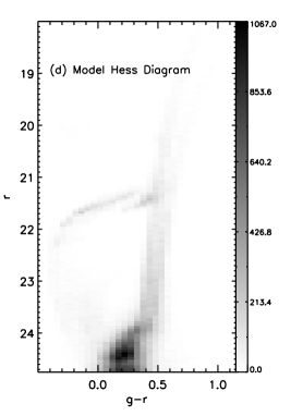
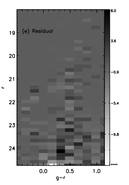
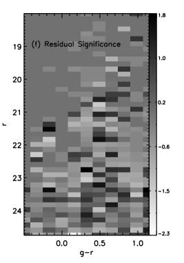
Figure 8.— Comparison of the data with our best StarFISH model fit. Pixel bins are 0.15 mag along the color and magnitude axis (except for panel (d), where the bins are 0.05 mag), as used in our StarFISH fits. The gray scale for each Hess diagram is in units of stars per pixel, except for panel (f), which has been scaled by the uncertainty associated with each pixel. (a) The observed Hess diagram of Leo IV within the half light radius. (b) The background Hess diagram, which was fit along with the theoretical isochrones. (c) The background-subtracted Hess diagram. (d) The best model CMD derived by StarFISH (with no background component), in bins of 0.05 mag in order to show the details of the model. (e) Residuals after subtracting a random realization of the StarFISH model from the data. (f) The residual from (e), scaled by the expected Poisson scatter in the bin. The most significant residuals are associated with the mismatch of the BHB between model and data.

The position of our high-probability blue plume (squares) and candidate BHB (diamonds) stars overplotted onto the smoothed map of Leo IV. Note that the probable blue plume stars are segregated within the body of Leo IV, as would be expected if they represented a young stellar population rather than blue straggler stars. As expected, there are few of these objects outside the main body of Leo IV. The BHB star population is more uniformly distributed across Leo IV.

The frequency of blue plume stars, normalized by BHB stars, for the MW dwarf spheroidals. The solid, circular points are the blue plume frequency points for the MW dwarfs derived by Momany et al. (2007). Note the anti-correlation between satellite brightness versus blue plume frequency. An outlier from that work is Carina, which likely harbors a young stellar population. The Canes Venatici I point is from Martin et al. (2008a) who reported a young stellar population in that system due to both the high blue plume frequency and the segregation of this population within the dwarf. Likewise, the blue plume frequency of Leo IV lies off the relation of Momany et al. (2007). That, along with the segregation seen in Figure A Deeper Look at Leo IV: Star Formation History and Extended Structure indicates that Leo IV harbors a small, young stellar population.

Comparison of the input ellipcity in our mock Leo IV dwarf galaxy models versus the output ellipticity found by our maximum likelihood algorithm. The points represent the median value of the 1000 bootstrap resamples, and the error bars represent the central 68.3% of the distribution around the median. The dashed line is the one-to-one correspondence between input and output. For input ellipticity values of $\epsilon_{input}\lesssim 0.25$ we systematically overpredict the ellipticity with large error bars and thus only quote upper limits.

Figure 9.— An illustration of how the maximum likelihood code for measuring parameterized structure performs for an input position angle of 35 degrees while varying the input ellipticity between 0.1 and 0.35. The output histograms are the results of the one thousand bootstrap resamples for the labeled scenarios, while the solid vertical line is the input value of the model, in this case PA = 35.0 degrees (top row) and $r_{h}=3.0$ arcmin (bottom row). Top row – Recovered position angle for various mock Leo IV models with $\epsilon$ between 0.1 and 0.35. Note how the example with an input ellipticity of $\epsilon$=0.10 does not have a clearly measured position angle, and the peak of the distribution does not agree with the model’s position angle. It is not until an ellipticity of $\epsilon\sim$0.35 where the model’s position angle is well measured and accurate. Bottom – Recovered half light radius while varying the input ellipticity. Although the low ellipticity case of $\epsilon=0.1$ seems to be slightly offset from the input $r_{h}=3.0$ arcmin model, the recovered half light radius is still within 1-$\sigma$ of the input value. In all other cases, the half light radius is measured with high precision.

Table 1Leo IV Photometry

Star No.	$\alpha$	$\delta$	$g$	$\delta g$	$A_{g}$	$r$	$\delta r$	$A_{r}$	SDSS or MMT
	(deg J2000.0)	(deg J2000.0)	(mag)	(mag)	(mag)	(mag)	(mag)	(mag)
0	173.23115	-0.54635	18.23	0.02	0.09	17.93	0.01	0.07	SDSS
1	173.24960	-0.50828	17.16	0.01	0.09	16.61	0.01	0.06	SDSS
2	173.20208	-0.54312	17.03	0.02	0.09	16.61	0.01	0.07	SDSS
3	173.22927	-0.49215	18.66	0.02	0.09	17.20	0.01	0.06	SDSS
4	173.25937	-0.50253	17.87	0.01	0.09	17.47	0.01	0.06	SDSS
5	173.19711	-0.49921	16.58	0.02	0.09	15.84	0.01	0.06	SDSS
6	173.21481	-0.58547	16.52	0.02	0.09	15.50	0.01	0.07	SDSS
7	173.23169	-0.47729	17.00	0.02	0.09	15.81	0.01	0.06	SDSS
8	173.23995	-0.60117	18.08	0.02	0.09	17.47	0.01	0.07	SDSS
9	173.19902	-0.56584	19.31	0.02	0.09	17.78	0.01	0.07	SDSS

Table 2Leo IV structure – parameterized fits

Parameter	Measured	Uncertainty	Bootstrap median
$M_{V}$	-5.5	0.3	-5.5
$\mu_{0,V}$	27.2	0.3	27.2
Exponential Profile
RA (h m s)	11:32:56.38	$\pm 14^{\prime\prime}$	11:32:56.33
DEC (d m s)	-00:32:27.25	$\pm 14^{\prime\prime}$	-00:32:29.24
$r_{h}$ (arcmin)	2.85	0.64	3.17
(pc)	127.8	28.8	142.2
$\epsilon$	0.05	$<0.23$	0.14
Plummer Profile
RA (h m s)	11:32:56.20	$\pm 12^{\prime\prime}$	11:32:56.18
DEC (d m s)	-00:32:27.17	$\pm 10^{\prime\prime}$	-00:32:28.32
$r_{h}$ (arcmin)	2.86	0.40	2.97
(pc)	128.1	18.0	133.3
$\epsilon$	0.02	$<0.20$	0.11
King Profile
RA (h m s)	11:32:56.04	$\pm 13^{\prime\prime}$	11:32:56.08
DEC (d m s)	-00:32:29.60	$\pm 10^{\prime\prime}$	-00:32:29.95
$r_{c}$ (arcmin)	1.61	0.22	1.64
(pc)	72.2	10.3	73.4
$r_{t}$ (arcmin)	18.55	4.39	20.25
(pc)	831.0	196.7	907.3
$\epsilon$	0.03	$<0.18$	0.09

Table 3Simulated Leo IV External Structures and Detections

No. of stars	$M_{r}$	$\mu_{0,r}$	$M_{g}$	$\mu_{0,g}$	Peak $\sigma$
Input ’Nuggets’
25	-1.0	29.7	-0.6	30.1	4.0
35	-2.8	27.9	-2.5	28.3	6.4
50	-3.2	27.5	-3.0	27.7	9.7
Input ’Streams’
100	-3.5	30.5	-3.2	30.8	1.7
200	-4.4	29.6	-4.3	29.8	4.3
300	-5.4	28.7	-5.0	29.0	5.1

References

- Adelman-McCarthy et al. (2006) Adelman-McCarthy, J. K., Agüeros, M. A., Allam, S. S., Anderson, K. S. J., Anderson, S. F., Annis, J., Bahcall, N. A., Baldry, I. K., Barentine, J. C., Berlind, A., Bernardi, M., Blanton, M. R., Boroski, W. N., Brewington, H. J., Brinchmann, J., Brinkmann, J., Brunner, R. J., Budavári, T., Carey, L. N., Carr, M. A., Castander, F. J., Connolly, A. J., Csabai, I., Czarapata, P. C., Dalcanton, J. J., Doi, M., Dong, F., Eisenstein, D. J., Evans, M. L., Fan, X., Finkbeiner, D. P., Friedman, S. D., Frieman, J. A., Fukugita, M., Gillespie, B., Glazebrook, K., Gray, J., Grebel, E. K., Gunn, J. E., Gurbani, V. K., de Haas, E., Hall, P. B., Harris, F. H., Harvanek, M., Hawley, S. L., Hayes, J., Hendry, J. S., Hennessy, G. S., Hindsley, R. B., Hirata, C. M., Hogan, C. J., Hogg, D. W., Holmgren, D. J., Holtzman, J. A., Ichikawa, S.-i., Ivezić, Ž., Jester, S., Johnston, D. E., Jorgensen, A. M., Jurić, M., Kent, S. M., Kleinman, S. J., Knapp, G. R., Kniazev, A. Y., Kron, R. G., Krzesinski, J., Kuropatkin, N., Lamb, D. Q., Lampeitl, H., Lee, B. C., Leger, R. F., Lin, H., Long, D. C., Loveday, J., Lupton, R. H., Margon, B., Martínez-Delgado, D., Mandelbaum, R., Matsubara, T., McGehee, P. M., McKay, T. A., Meiksin, A., Munn, J. A., Nakajima, R., Nash, T., Neilsen, Jr., E. H., Newberg, H. J., Newman, P. R., Nichol, R. C., Nicinski, T., Nieto-Santisteban, M., Nitta, A., O’Mullane, W., Okamura, S., Owen, R., Padmanabhan, N., Pauls, G., Peoples, J. J., Pier, J. R., Pope, A. C., Pourbaix, D., Quinn, T. R., Richards, G. T., Richmond, M. W., Rockosi, C. M., Schlegel, D. J., Schneider, D. P., Schroeder, J., Scranton, R., Seljak, U., Sheldon, E., Shimasaku, K., Smith, J. A., Smolčić, V., Snedden, S. A., Stoughton, C., Strauss, M. A., SubbaRao, M., Szalay, A. S., Szapudi, I., Szkody, P., Tegmark, M., Thakar, A. R., Tucker, D. L., Uomoto, A., Vanden Berk, D. E., Vandenberg, J., Vogeley, M. S., Voges, W., Vogt, N. P., Walkowicz, L. M., Weinberg, D. H., West, A. A., White, S. D. M., Xu, Y., Yanny, B., Yocum, D. R., York, D. G., Zehavi, I., Zibetti, S., & Zucker, D. B. 2006, ApJS, 162, 38
- Belokurov et al. (2008) Belokurov, V., Walker, M. G., Evans, N. W., Faria, D. C., Gilmore, G., Irwin, M. J., Koposov, S., Mateo, M., Olszewski, E., & Zucker, D. B. 2008, ApJ, 686, L83
- Belokurov et al. (2007) Belokurov, V., Zucker, D. B., Evans, N. W., Kleyna, J. T., Koposov, S., Hodgkin, S. T., Irwin, M. J., Gilmore, G., Wilkinson, M. I., Fellhauer, M., Bramich, D. M., Hewett, P. C., Vidrih, S., De Jong, J. T. A., Smith, J. A., Rix, H.-W., Bell, E. F., Wyse, R. F. G., Newberg, H. J., Mayeur, P. A., Yanny, B., Rockosi, C. M., Gnedin, O. Y., Schneider, D. P., Beers, T. C., Barentine, J. C., Brewington, H., Brinkmann, J., Harvanek, M., Kleinman, S. J., Krzesinski, J., Long, D., Nitta, A., & Snedden, S. A. 2007, ApJ, 654, 897
- Coleman et al. (2004) Coleman, M., Da Costa, G. S., Bland-Hawthorn, J., Martínez-Delgado, D., Freeman, K. C., & Malin, D. 2004, AJ, 127, 832
- Coleman et al. (2005) Coleman, M. G., Da Costa, G. S., Bland-Hawthorn, J., & Freeman, K. C. 2005, AJ, 129, 1443
- Coleman et al. (2007) Coleman, M. G., de Jong, J. T. A., Martin, N. F., Rix, H.-W., Sand, D. J., Bell, E. F., Pogge, R. W., Thompson, D. J., Hippelein, H., Giallongo, E., Ragazzoni, R., DiPaola, A., Farinato, J., Smareglia, R., Testa, V., Bechtold, J., Hill, J. M., Garnavich, P. M., & Green, R. F. 2007, ApJ, 668, L43
- Davies et al. (2004) Davies, M. B., Piotto, G., & de Angeli, F. 2004, MNRAS, 349, 129
- de Jong et al. (2008a) de Jong, J. T. A., Harris, J., Coleman, M. G., Martin, N. F., Bell, E. F., Rix, H.-W., Hill, J. M., Skillman, E. D., Sand, D. J., Olszewski, E. W., Zaritsky, D., Thompson, D., Giallongo, E., Ragazzoni, R., DiPaola, A., Farinato, J., Testa, V., & Bechtold, J. 2008a, ApJ, 680, 1112
- de Jong et al. (2008b) de Jong, J. T. A., Rix, H.-W., Martin, N. F., Zucker, D. B., Dolphin, A. E., Bell, E. F., Belokurov, V., & Evans, N. W. 2008b, AJ, 135, 1361
- de Jong et al. (2010) de Jong, J. T. A., Yanny, B., Rix, H., Dolphin, A. E., Martin, N. F., & Beers, T. C. 2010, ApJ, 714, 663
- de Marchi et al. (2006) de Marchi, F., de Angeli, F., Piotto, G., Carraro, G., & Davies, M. B. 2006, A&A, 459, 489
- Dolphin (2002) Dolphin, A. E. 2002, MNRAS, 332, 91
- Geha et al. (2009) Geha, M., Willman, B., Simon, J. D., Strigari, L. E., Kirby, E. N., Law, D. R., & Strader, J. 2009, ApJ, 692, 1464
- Girardi et al. (2004) Girardi, L., Grebel, E. K., Odenkirchen, M., & Chiosi, C. 2004, A&A, 422, 205
- Gnedin & Kravtsov (2006) Gnedin, N. Y. & Kravtsov, A. V. 2006, ApJ, 645, 1054
- Grcevich & Putman (2009) Grcevich, J. & Putman, M. E. 2009, ApJ, 696, 385
- Harris & Zaritsky (2001) Harris, J. & Zaritsky, D. 2001, ApJS, 136, 25
- Harris & Zaritsky (2009) —. 2009, AJ, 138, 1243
- Hurley-Keller et al. (1998) Hurley-Keller, D., Mateo, M., & Nemec, J. 1998, AJ, 115, 1840
- King (1966) King, I. R. 1966, AJ, 71, 64
- Kirby et al. (2008) Kirby, E. N., Simon, J. D., Geha, M., Guhathakurta, P., & Frebel, A. 2008, ApJ, 685, L43
- Klessen et al. (2003) Klessen, R. S., Grebel, E. K., & Harbeck, D. 2003, ApJ, 589, 798
- Mapelli et al. (2009) Mapelli, M., Ripamonti, E., Battaglia, G., Tolstoy, E., Irwin, M. J., Moore, B., & Sigurdsson, S. 2009, MNRAS, 396, 1771
- Mapelli et al. (2007) Mapelli, M., Ripamonti, E., Tolstoy, E., Sigurdsson, S., Irwin, M. J., & Battaglia, G. 2007, MNRAS, 380, 1127
- Martin et al. (2008a) Martin, N. F., Coleman, M. G., De Jong, J. T. A., Rix, H., Bell, E. F., Sand, D. J., Hill, J. M., Thompson, D., Burwitz, V., Giallongo, E., Ragazzoni, R., Diolaiti, E., Gasparo, F., Grazian, A., Pedichini, F., & Bechtold, J. 2008a, ApJ, 672, L13
- Martin et al. (2008b) Martin, N. F., de Jong, J. T. A., & Rix, H.-W. 2008b, ApJ, 684, 1075
- Mateo et al. (1995) Mateo, M., Fischer, P., & Krzeminski, W. 1995, AJ, 110, 2166
- McLeod et al. (2000) McLeod, B. A., Conroy, M., Gauron, T. M., Geary, J. C., & Ordway, M. P. 2000, in Further Developments in Scientific Optical Imaging, ed. M. B. Denton, 11–+
- Momany et al. (2007) Momany, Y., Held, E. V., Saviane, I., Zaggia, S., Rizzi, L., & Gullieuszik, M. 2007, A&A, 468, 973
- Monelli et al. (2003) Monelli, M., Pulone, L., Corsi, C. E., Castellani, M., Bono, G., Walker, A. R., Brocato, E., Buonanno, R., Caputo, F., Castellani, V., Dall’Ora, M., Marconi, M., Nonino, M., Ripepi, V., & Smith, H. A. 2003, AJ, 126, 218
- Moretti et al. (2009) Moretti, M. I., Dall’Ora, M., Ripepi, V., Clementini, G., Di Fabrizio, L., Smith, H. A., DeLee, N., Kuehn, C., Catelan, M., Marconi, M., Musella, I., Beers, T. C., & Kinemuchi, K. 2009, ApJ, 699, L125
- Munoz et al. (2009) Munoz, R. R., Geha, M., & Willman, B. 2009, ArXiv 0910.3946, AJ submitted
- Olszewski et al. (2006) Olszewski, E. W., Mateo, M., Harris, J., Walker, M. G., Coleman, M. G., & Da Costa, G. S. 2006, AJ, 131, 912
- Olszewski et al. (1996) Olszewski, E. W., Suntzeff, N. B., & Mateo, M. 1996, ARA&A, 34, 511
- Peñarrubia et al. (2009) Peñarrubia, J., Walker, M. G., & Gilmore, G. 2009, MNRAS, 399, 1275
- Piotto et al. (2004) Piotto, G., De Angeli, F., King, I. R., Djorgovski, S. G., Bono, G., Cassisi, S., Meylan, G., Recio-Blanco, A., Rich, R. M., & Davies, M. B. 2004, ApJ, 604, L109
- Plummer (1911) Plummer, H. C. 1911, MNRAS, 71, 460
- Press et al. (1988) Press, W. H., Flannery, B. P., Teukolsky, S. A., & Vetterling, W. T. 1988, Numerical recipes in C: the art of scientific computing (New York, NY, USA: Cambridge University Press)
- Ricotti (2009) Ricotti, M. 2009, MNRAS, 392, L45
- Ricotti & Gnedin (2005) Ricotti, M. & Gnedin, N. Y. 2005, ApJ, 629, 259
- Ryan-Weber et al. (2008) Ryan-Weber, E. V., Begum, A., Oosterloo, T., Pal, S., Irwin, M. J., Belokurov, V., Evans, N. W., & Zucker, D. B. 2008, MNRAS, 384, 535
- Sand et al. (2009) Sand, D. J., Olszewski, E. W., Willman, B., Zaritsky, D., Seth, A., Harris, J., Piatek, S., & Saha, A. 2009, ApJ, 704, 898
- Sandage & Cacciari (1990) Sandage, A. & Cacciari, C. 1990, ApJ, 350, 645
- Schlegel et al. (1998) Schlegel, D. J., Finkbeiner, D. P., & Davis, M. 1998, ApJ, 500, 525
- Simon & Geha (2007) Simon, J. D. & Geha, M. 2007, ApJ, 670, 313
- Stetson (1994) Stetson, P. B. 1994, PASP, 106, 250
- Walker et al. (2009) Walker, M. G., Belokurov, V., Evans, N. W., Irwin, M. J., Mateo, M., Olszewski, E. W., & Gilmore, G. 2009, ApJ, 694, L144
- Walsh et al. (2008) Walsh, S. M., Willman, B., Sand, D., Harris, J., Seth, A., Zaritsky, D., & Jerjen, H. 2008, ApJ, 688, 245
- Willman (2010) Willman, B. 2010, Advances in Astronomy, 2010
- Zucker et al. (2006) Zucker, D. B., Belokurov, V., Evans, N. W., Kleyna, J. T., Irwin, M. J., Wilkinson, M. I., Fellhauer, M., Bramich, D. M., Gilmore, G., Newberg, H. J., Yanny, B., Smith, J. A., Hewett, P. C., Bell, E. F., Rix, H.-W., Gnedin, O. Y., Vidrih, S., Wyse, R. F. G., Willman, B., Grebel, E. K., Schneider, D. P., Beers, T. C., Kniazev, A. Y., Barentine, J. C., Brewington, H., Brinkmann, J., Harvanek, M., Kleinman, S. J., Krzesinski, J., Long, D., Nitta, A., & Snedden, S. A. 2006, ApJ, 650, L41