BOO–1137 – AN EXTREMELY METAL-POOR STAR IN THE ULTRA–FAINT DWARF SPHEROIDAL GALAXY BOÖTES I

Abstract

We present high-resolution (R $\sim$ 40000), high-$S/N$ (20–90) spectra of an extremely metal-poor giant star Boo$-$1137 in the “ultra-faint” dwarf spheroidal galaxy (dSph) Boötes I, absolute magnitude M${}_{V}\sim-6.3$. We derive an iron abundance of [Fe/H] = –3.7, making this the most metal-poor star as yet identified in an ultra-faint dSph. Our derived effective temperature and gravity are consistent with its identification as a red giant in Boötes I.

Abundances for a further 15 elements have also been determined. Comparison of the relative abundances, [X/Fe], with those of the extremely metal-poor red giants of the Galactic halo shows that Boo$-$1137 is “normal” with respect to C and N, the odd-Z elements Na and Al, the iron-peak elements, and the neutron-capture elements Sr and Ba, in comparison with the bulk of the Milky Way halo population having [Fe/H] $\lesssim$ –3.0. The $\alpha$-elements Mg, Si, Ca, and Ti are all higher by $\Delta$[X/Fe] $\sim$ 0.2 than the average halo values. Monte-Carlo analysis indicates that $\Delta$[$\alpha$/Fe] values this large are expected with a probability $\sim$ 0.02. The elemental abundance pattern in Boo–1137 suggests inhomogeneous chemical evolution, consistent with the wide internal spread in iron abundances we previously reported. The similarity of most of the Boo$-$1137 relative abundances with respect to halo values, and the fact that the $\alpha$-elements are all offset by a similar small amount from the halo averages, points to the same underlying galaxy-scale stellar initial mass function, but that Boo$-$1137 likely originated in a star-forming region where the abundances reflect either poor mixing of supernova ejecta, or poor sampling of the supernova progenitor mass range, or both.

1 INTRODUCTION

The discovery and analysis of extremely metal-poor stars (those with [Fe/H]  $<$ –3.0) in extremely low luminosity dwarf spheroidal galaxies is changing our perspective on the early chemical enrichment within these objects, the formation of the outer regions of the Milky Way halo, and the role of dwarf spheroidal galaxies (dSph) within the $\Lambda$CDM paradigm of the manner in which the Milky Way formed.

Initial observations of the brighter dSph (Helmi et al. 2006, and references therein) led to the conclusion that dSph contained no stars with [Fe/H] $<$ –3.0, while detailed studies of relative abundances (in particular [$\alpha$/Fe]) showed patterns that were unlike those of Galactic halo stars in the solar neighborhood (Venn et al. 2004, and references therein; see also Tolstoy, Hill, & Tosi 2009). The paucity of brighter Milky Way dSph and their chemical relative abundances seem at odds with the CDM paradigm (Klypin et al. 1999; Moore et al. 1999) and the concept that these systems are the building blocks of at least part of the Galaxy’s halo. The recent identification of several “ultra-faint” systems, with luminosities many orders of magnitude fainter than those of the classical dSph, through analyses of the imaging data from the Sloan Digital Sky Survey (e.g. Belokurov et al. 2006, 2007) has revitalized discussions of satellite luminosity and mass functions. Further, these ultra-faint systems contain extremely low-metallicity stars (Kirby et al. 2008; Norris et al. 2008), perhaps redressing the apparent deficit in brighter dSph. Arguably even more interesting than their relevance as building blocks is to understand the galaxies themselves. Are they the first objects? Did they cause reionization? What do they tell us of the first stars? What was the stellar Initial Mass Function (IMF) at near zero metallicity? How are the faintest dSph related to more luminous dSph and the Milky Way?

In a study of several ultra-faint dSph, Kirby et al. (2008) first reported stars with [Fe/H] $<-3.0$ (with metallicities as low as [Fe/H] $=-3.3$), based on moderate-resolution spectra in the range 8300–8500 Å, while Norris et al. (2008) from multi-object spectroscopy of the Boötes I dSph found a similar result, with the most metal-poor star having [Fe/H] $=-3.4$ based on the CaII K line (3933 Å) in moderate resolution blue spectra. More recently, Frebel et al. (2009) have obtained the first detailed elemental abundances, based on high-resolution, high $S/N$ spectra, of extremely metal-poor stars in the ultra-faint systems, with observations of Com Ber and U Ma II (M${}_{V}\sim-4,\,-5.5$ respectively). Of the six stars studied, one has [Fe/H] $=-3.2$, and another $-3.1$. Perhaps the most interesting result of their investigation is that in these stars [$\alpha$/Fe] is similar to that found in the bulk of Galactic halo stars. That is to say, these low metallicity stars in these faint satellite galaxies were apparently enriched by SNe from a similar stellar IMF to that which enriched their Milky Way counterparts. The most metal-poor – and possibly oldest – stars in the more luminous dSph also show the same level of enhancement of the $\alpha$-elements (e.g. Koch et al. 2008). These results stand in some contrast to results at higher abundance, in which regime the dSph member stars have significantly lower levels of [$\alpha$/Fe] than seen in field halo stars of the same iron abundance (e.g. Venn et al. 2004), plausibly reflecting the more extended star formation and self-enrichment in the dSph in contrast to the field halo (Unavane, Wyse & Gilmore 1996). The ultra-faint systems have sufficiently low luminosities and low metallicities that one might observe the anticipated signatures of enrichment by single Type II supernovae, perhaps even by Population III massive stars.

The Boötes I system was discovered by Belokurov et al. (2006) and is an ultra-faint dSph (M${}_{V}\sim-6.3$, luminosity $\sim 3\times 10^{4}$ L_⊙; Martin et al. 2008) at a distance of $\sim 65$ kpc. The observed color-magnitude diagram is consistent with an old, metal-poor system. We identified extremely metal-poor member stars in Boötes I, together with a large internal dispersion in metallicity, through intermediate-resolution spectroscopy of the Ca II H and K lines (Norris et al. 2008). We here report follow-up, high-resolution, high-S/N, observations of the particularly interesting star Boo$-$1137 we identified which lies at $\sim 2$ half-light radii from the center of Boötes I, and for which we had derived [Fe/H] = –3.4. In §2 we present data obtained for this star using the VLT/UVES system with resolving power R = 40000 and $S/N$ = 20–90. In §3 we report chemical abundances from a model atmosphere analysis of this material for some 16 elements. Boo$-$1137 has [Fe/H] = –3.7, and relative abundances ([X/Fe]) that are very similar to those of Galactic halo stars of the same [Fe/H]. We discuss the implications of our results in §4.

2 OBSERVATIONS AND REDUCTION

2.1 $ugriz$ Photometry

Boo$-$1137 lies at $\alpha(2000)=13$ h $58$ m $33.8$ s and $\delta(2000)=+14^{\circ}\;21^{\prime}\;08^{\prime\prime}$. $ugriz$ photometry is available from Data Release 7 of the Sloan Digital Sky Survey (Abazajian et al. 2009, http://cas.sdss.org/astrodr7/en/tools/search/). Following Belokurov et al. (2006), we adopt E(B–V) = 0.02 (and hence E(g–r) = 0.021 and E(r–z) = 0.027 (see Schlegel, Finkbeiner, & Davis 1998)), to obtain (g–r)₀ = 0.718 $\pm$ 0.009 and (r–z)₀ = 0.518 $\pm$ 0.011 for Boo$-$1137. We also use the transformation (B–V)₀ = 1.197$\times$(g–r)₀ + 0.049, appropriate for metal-poor red giants (Norris et al. 2008), to obtain (B–V)₀ = 0.91 $\pm$ 0.01. These are used in the abundance analysis in §3.1.

2.2 High-resolution Spectroscopy

Boo$-$1137 was observed in Service Mode at the Very Large Telescope (VLT) Unit Telescope 2 (UT2) with the Ultraviolet-Visual Echelle Spectrograph (UVES) (Dekker et al. 2000, http://www.eso.org/sci/facilities/paranal/instruments/uves/) during the nights of 2009 April 24 and 25. Ten individual exposures with an integration time of 46 min each were obtained. UVES was used in dichroic mode with the BLUE390 and RED564 settings, covering the wavelength ranges 3300–4520 Å in the blue-arm spectra, and 4620–5600 Å and 5680–6650 Å in the lower- and upper- red-arm spectra, respectively. A 1 ″ wide slit was used for all observations.

The ten pipeline-reduced spectra were co-added to produce the final results. The co-added blue-arm spectrum has a maximum $S/N$ per $0.027$ Å pixel $\sim$ $40$ at $4500$ Å, decreasing to $S/N\sim 30$ at $4100$ Å and $S/N\sim 20$ at $3700$ Å. Below $3700$ Å, the spectrum is only of limited usefulness. In the lower red-arm spectrum, the $S/N$ per $0.028$ Å pixel was $\sim$ 60 throughout, while for the upper red-arm spectrum the $S/N$ per $0.033$ Å pixel increases from 70 to 90.

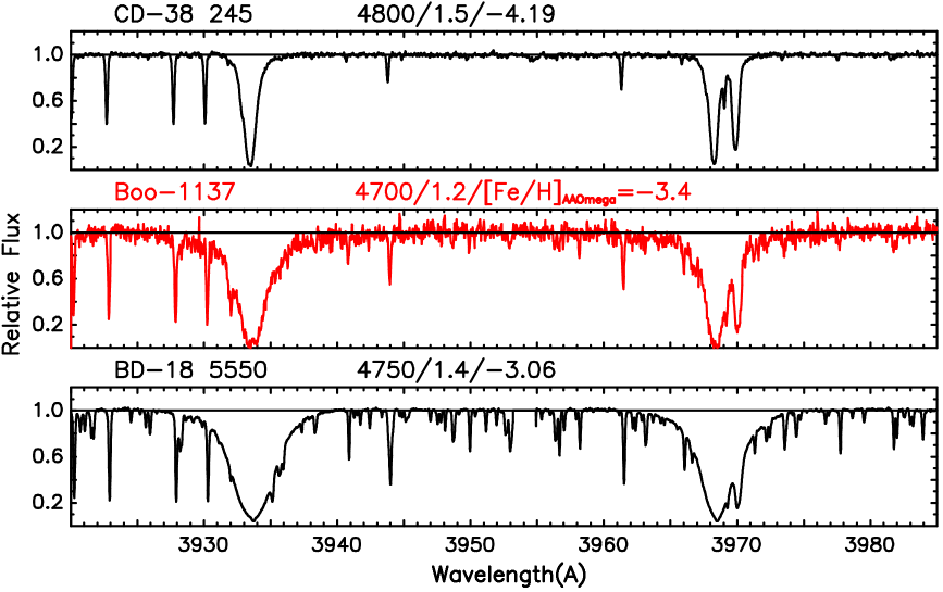
Figure 1: Comparison of the spectrum of Boo$-$1137 in the region of the Ca II H and K lines with those of the metal-poor giants CD$-38^{\circ}\,245$ ([Fe/H] = –4.2) and BD$-18^{\circ}\,5550$ ([Fe/H] = –3.1). The atmospheric parameters $T_{\rm eff}$/log $g$/[Fe/H] (from Cayrel et al. (2004) and §3 of the present work (except for [Fe/H], which comes from Norris et al. 2008)) are also presented above each spectrum. Note that Boo$-$1137 has line strengths, and thus abundances, intermediate between those of the two comparison objects.

An example of the continuum normalized spectrum of Boo$-$1137 in the region of the Ca II K line is shown in Figure 1, where it is compared with those of the extremely metal-poor giants CD$-38^{\circ}\,245$ and BD$-18^{\circ}\,5550$ which have effective temperatures and gravities similar to those of Boo$-$1137, and abundances [Fe/H] = –4.2 and –3.1, respectively. Inspection of the figure suggests that Boo$-$1137 does indeed have an abundance consistent with our initial estimate of [Fe/H] = –3.4.

2.3 Line Strength Measurements

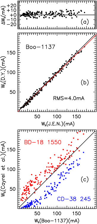
Figure 2: (a,b) Comparison of equivalent widths measured by D.Y. and J.E.N. in the VLT/UVES spectrum of Boo$-$1137. ((b) contains the linear least squares best fit and 1–1 lines, while in (a) $\Delta$W_λ = W_λ(J.E.N.) – W_λ(D.Y.).) (c) The equivalent widths of CD$-38^{\circ}\,245$ ([Fe/H] = –4.2) and BD$-18^{\circ}\,5550$ ([Fe/H] = –3.1) (from Cayrel et al. 2004) versus the present results for Boo$-$1137. Note that the line strengths in CD$-38^{\circ}\,245$ and BD$-18^{\circ}\,5550$ are smaller and larger, respectively, than in Boo$-$1137.

Beginning with the line list of Cayrel et al. (2004), supplemented by four (non-Fe I) lines that appear unblended in the Sun and Arcturus and have log $gf$ values in the Vienna Atomic Line Database (VALD)(Kupka et al. 1999), we have used the VLT spectra to measure equivalent widths of 14 elements in Boo$-$1137 in the wavelength range 3800–6650 Å. (Two further elements, C and N, are discussed below.) A comparison of independent line strength determinations by the first two authors obtained using techniques described by Norris et al. (2001) and Yong et al. (2008) is shown in Figure 2a,b, where the agreement is quite satisfactory, with an RMS scatter between the two estimates of 4.0 mÅ. While a small departure from the one-to-one line is evident in the figure, representing a systematic difference of a few mÅ, we have chosen to average the data, and present in column (5) of Table 1 line strengths for 152 unblended lines suitable for model atmosphere abundance analysis. Lower excitation potentials, $\chi$, and log $gf$ values are presented in columns (3) and (4) of the table, taken preferentially from Table 3 of Cayrel et al. (2004), and supplemented by material from the VALD database.

For heuristic purposes we also show, in Figure 2c, the line strengths of CD$-38^{\circ}\,245$ ([Fe/H] = –4.2) and BD$-18^{\circ}\,5550$ ([Fe/H] = –3.1) versus those of Boo$-$1137. As one might expect from the comparisons presented in Figure 1, and recalling that the three objects have similar effective temperatures and gravities, Boo$-$1137 has line strengths intermediate between those of CD$-38^{\circ}\,245$ and BD$-18^{\circ}\,5550$.

2.4 Radial Velocity

Radial velocities for Boo$-$1137 were measured (over the wavelength range 5160–5190 Å) by Fourier cross-correlation (using routines in the FIGARO reduction package
(see http://www.aao.gov.au/figaro) of each of its ten pipeline reduced spectra against a synthetic spectrum having $T_{\rm eff}$ = 4700K, log $g$ = 1.5, [M/H] = –3.5, and microturbulent velocity $\xi_{t}$ = 2 km s^-1 (computed with the code described by Cottrell and Norris 1978, and atomic line wavelengths from VALD). The resulting heliocentric velocity is V_r = 99.1 $\pm$ 0.1 km s^-1, with the individual velocities covering the range 98.8–99.5 km s^-1. The quoted error is the standard error on the mean, and refers to the internal error of measurement, and does not include any consideration of the external error, given that spectra of velocity standards were not obtained as part of this program. Lucatello et al. (2005) find, from a careful study of the metal-poor subgiant HD 140283, that the external error for UVES is 0.3 km s^-1, while Napiwotzki et al., in a private communication to Norris et al. (2007), report a value of 0.7 km s^-1. For the purposes of the present investigation we shall adopt an external error of 0.5 km s^-1, the mean of these two estimates.

When internal and external errors are taken together, we thus have V_r = 99.1 $\pm$ 0.5 km s^-1 for Boo$-$1137, which is consistent with radial velocity membership of Boötes I, for which Martin et al. (2007) report a systemic velocity of 95.6 $\pm$ 3.4 km s^-1 and dispersion of 6.6 $\pm$ 2.3 km s^-1. It also agrees with the previous value reported for this star by Norris et al. (2008), when their cited value is placed on the system of Martin et al. (by requiring that the mean velocities of the two investigations agree), which then becomes 104 $\pm$ 7 km s^-1.

3 ABUNDANCE ANALYSIS

3.1 Effective Temperature and Surface Gravity

$T_{\rm eff}$ and log $g$ were determined from (g–r)₀ and (r–z)₀ by assuming that Boo$-$1137 lies on the red giant branch and iteratively using the synthetic $ugriz$ colors of Castelli
(http://wwwuser.oat.ts.astro.it/castelli/colors/sloan.html) and the Yale–Yonsei Isochrones (Demarque at al. 2004, http://www.astro.yale.edu/demarque/yyiso.html), with an age of 12 Gyr. Similarly, the (B–V)₀ value for Boo$-$1137 was used together with these isochrones to provide another estimate of the parameters. The process required a knowledge of the chemical abundance. In practice, first estimates of $T_{\rm eff}$ and log $g$, based on the initial value of [Fe/H] = –3.4 from Norris et al. (2008), were adopted in the model atmosphere abundance analysis described below, and an iterative procedure followed using the new value of [Fe/H], until convergence was obtained. This happened after one iteration. The individual values of $T_{\rm eff}$ and log $g$ lie in the ranges 4640–4760K and 1.0–1.3 dex, respectively. Our final adopted values are $T_{\rm eff}$ = 4700K and log $g$ = 1.2. It is difficult to estimate the systematic errors in these parameters: in what follows we shall somewhat arbitrarily adopt $\Delta$$T_{\rm eff}$ = 200K and $\Delta$log $g$ = 0.3.

3.2 Relative Abundances from Atomic Features

We determined the abundance of key elements beginning with iron – the canonical measure of metallicity. Model atmospheres were taken from the NEWODF grid of ATLAS9 models (plane-parallel, one-dimensional (1D), local thermodynamic equilibrium (LTE)) of Castelli & Kurucz (2003, http://wwwuser.oat.ts.astro.it/castelli/grids.html). The particular grid of models used was $\alpha$-enhanced, [$\alpha$/Fe] = +0.4, and computed assuming a microturbulent velocity of $\xi_{t}$ = 2 km s^-1. Interpolation within the grid was performed when necessary to produce models with the required $T_{\rm eff}$, log $g$, and [M/H]. The interpolation software, kindly provided by Dr Carlos Allende Prieto, has been used extensively (e.g., Reddy et al. 2003 and Allende Prieto et al. 2004).

The model atmospheres were used in conjunction with two versions of the LTE stellar line analysis program MOOG (Sneden 1973). The first was the 2009 standard version then available at http://verdi.as.utexas.edu/moog.html, while the second is currently under development, and uses a more rigorous treatment of continuum scattering. The latter version was generously made available to us by Prof. Chris Sneden. We tested both versions by analyzing the equivalent widths of the 35 metal-poor stars of Cayrel et al. (2004), for lines having $\lambda\gtrsim$ 3750 Å. Adopting their atmospheric parameters, we found small but significant convergence in our abundances compared with theirs, when using the more recent version. That is to say, the agreement between our and their abundances went from very good to excellent. In what follows, therefore, we shall present results obtained by using the newer version of the code. This will prove useful in §4.2, where we shall compare our abundances for Boo$-$1137 with those for the Galactic halo giants of Cayrel et al. (2004). We shall comment below on the abundance differences that resulted, for the set of lines that we analyzed, between the two versions.

The microturbulent velocity, $\xi_{t}$, was determined in the usual way by requiring the abundances from Fe i lines to be independent of their reduced equivalent width, log($W_{\lambda}$/$\lambda$). For Boo$-$1137 we obtain $\xi_{t}$ = 2.2 $\pm$ 0.1 km s^-1. Determination of the Fe abundance offers a check on the adopted stellar parameters and the assumptions underlying the model atmospheres and line analysis, principally via the ionization and excitation balance. Concerning ionization equilibrium, the mean Fe abundances derived from neutral lines and from ionized lines provide a check on the adopted surface gravity. Additionally, differences between the abundances from Fe i and Fe ii lines may represent departures from LTE (e.g. Thevénin & Idiart 1999; but see also Gratton et al. 1999). For Boo$-$1137, these abundances agree within 0.06 dex, i.e., ionization equilibrium is satisfied, and this suggests our surface gravity is appropriate and departures from LTE are small.

Regarding excitation equilibrium, we note that other studies of metal-poor giants have reported a systematic trend between the abundance from Fe i lines and lower excitation potential, $\chi$, (e.g., Cayrel et al. 2004, Lai et al. 2008, and Cohen et al. 2008). Cayrel et al. (2004) and Lai et al. (2008) found that the trend between abundances from Fe i lines and lower excitation potential is alleviated, or indeed removed, by excluding lines with $\chi<$ 1.2 eV. In our analysis, we also find a trend between the abundances from Fe i lines and lower excitation potential when considering all lines – with slope $-$0.12 dex/eV, which is compatible in both sign and magnitude with the (lower) values reported by Lai et al. (2008). When considering only lines with $\chi>$ 1.2 eV, however, there is no statistically significant trend (even at the 1$\sigma$ level), as reported in previous studies.

Having performed these validity checks and obtained a measure of the microturbulent velocity, we then computed abundances for atomic features with measured equivalent widths using the adopted model atmosphere and MOOG. Some further details should, however, be noted. First, lines of Sc ii, Mn i, and Co i are affected by hyperfine splitting (HFS). In our abundance analysis, HFS was treated appropriately using the parameters from Kurucz & Bell (1995). In the case of Mn, Cayrel et al. (2004) also noted that the resonance triplet $a^{6}{\rm S}-z^{6}{\rm P}^{0}$ at 403 nm yields abundances systematically too low by 0.4 dex compared with results from other Mn lines. We have thus increased the Mn abundances in Tables 1 and 2, and throughout this work, by that amount. Finally, for the elements O, Zn and Eu, which are not measurable in our spectra, but which are observed at higher metallicity and have particular significance in comparison with models of galactic chemical enrichment, we computed abundance limits based on the O i 6300.30 Å, Zn i 4810.53 Å, and Eu ii 4129.72 Å lines, respectively, by adopting upper limit equivalent widths of 10 m Å.

Our abundances are presented in Table 2, where columns (1)–(5) contain the species, the number of lines measured (or, alternatively, that synthetic spectra were compared with observations), log($\epsilon$(X)), its error, and relative abundance [X/Fe], respectively. (In order to compute the relative abundances we adopted the solar abundance data of Asplund et al. (2005)). While we present abundances obtained using the revised version of MOOG, discussed above, in Table 2, we note that for our set of equivalent widths (with $\lambda\gtrsim$ 3750 Å), the revised version produces a value of [Fe/H] lower than the standard version by 0.03 dex, and relative abundances lower on average by 0.02 dex for the 16 species studied. As expected, the difference increases as one goes to shorter wavelength. For the atomic lines discussed here, the largest difference was –0.09 dex, for Al I, for which we observed only two lines – at 3944.00Å and 3968.52Å.

It will be important in the discussion of relative abundances in §4.2 to appreciate the systematic differences between the abundances presented here and those of Cayrel et al. (2004). In order to do this, we analyzed the equivalent width data in Table 3 of Cayrel et al.  adopting their atmospheric parameters, and using our techniques. For stars having [Fe/H] $<$ –3.0, the comparison of the log $\epsilon$ values for the atomic species in Table 8 of Cayrel et al. (2004) with our results (in the sense [Cayrel et al. – present work]) produces the following mean abundance differences: $\Delta$[Fe/H] = 0.023 $\pm$ 0.003, $\Delta$[Na I/Fe] = –0.071 $\pm$ 0.040, $\Delta$[Mg I/Fe] = –0.049 $\pm$ 0.007, $\Delta$[Al I/Fe] = –0.030 $\pm$ 0.009, $\Delta$[Ca I/Fe] = –0.008 $\pm$ 0.006, $\Delta$[Sc II/Fe] = –0.012 $\pm$ 0.009, $\Delta$[Ti I/Fe] = 0.033 $\pm$ 0.004, $\Delta$[Ti II/Fe] = –0.019 $\pm$ 0.006, $\Delta$[Cr I/Fe] = –0.001 $\pm$ 0.003, $\Delta$Fe II/Fe] = –0.027 $\pm$ 0.007, $\Delta$[Co I/Fe] = 0.005 $\pm$ 0.002, $\Delta$[Ni/Fe] = 0.016 $\pm$ 0.0.003. We regard this agreement, which is independent of adopted solar abundances, as very satisfactory.

We conclude this section by noting that abundances of both neutral and singly ionized lines of Ti are presented in the table, and permit a further check of the surface gravity and the presence of departures from LTE. One finds that abundances for the two ionization states agree within 0.08 dex, which, given their relative uncertainties, we regard as agreement (see section §3.4 on error analysis).

3.3 Relative Abundances from Molecular Features

Our spectra for Boo$-$1137 include features of CH and NH, which permit us to determine the abundances of carbon and nitrogen. For carbon, we compared observed and synthetic spectra (generated with MOOG) of the (0,0) and (1,1) bands of the $A-X$ electronic transition of the CH molecule in the interval 4250–4330 Å, while for nitrogen we used the (0,0) and (1,1) bands of the $A-X$ electronic transition of the NH molecule in the range 3340–3400 Å. (As noted above in §2.2, the $S/N$ is relatively poor in the latter wavelength range, which is reflected in the lower accuracy of our deduced nitrogen abundance.)

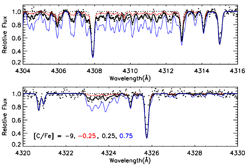
Figure 3: Comparison of the spectrum of Boo$-$1137 (heavy black dots) in the regions 4304–4316 Å (upper panel) and 4320–4330 Å (lower panel) with synthetic spectra including CH A–X lines for relative carbon abundances [C/Fe] = –9.0 (thin dotted line), –0.25 (thin red line), 0.25 (thick line; best fit), and 0.75 (thin blue line)

For carbon, we used the Plez et al. (2008) line list, and a dissociation energy of 3.465 eV. The abundance of C is weakly dependent on the assumed O abundance: since we have only an upper limit to the latter, the synthetic spectra were computed using the upper limit in Table 2, ([O/Fe] $<1.94$) and also with [O/Fe] = +0.5, consistent with the values observed in Galactic halo stars. For this range of O abundance, the inferred C abundance does not change. We adjusted the abundance of C until the synthetic spectrum matched the observed one, as may be seen in Figure 3. We find [C/Fe] = 0.25 $\pm$ 0.2 for Boo$-$1137.

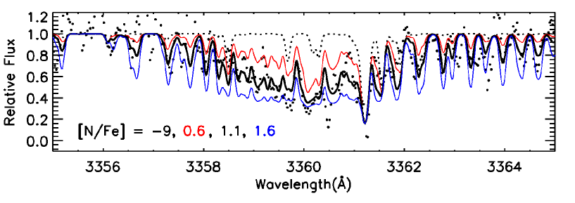
Figure 4: The spectrum of Boo$-$1137 (heavy black dots) in the region of NH A–X band at 3360 Å, compared with synthetic spectra having relative abundances [N/Fe] = –9.0 (thin dotted line), 0.6 (thin red line), 1.1 (thick line; best fit), and 1.6 (thin blue line).

For nitrogen, the line list was taken from Johnson et al. (2007), in which the Kurucz-$gf$ values were reduced by a factor of 2. We also adopted the dissociation potential of 3.450 eV. Given the poorer $S/N$ noted above, the observed spectrum was smoothed with a 5-pixel boxcar function to increase the signal-to-noise ratio. Figure 4 shows the comparison between observed and synthetic spectra, from which we infer [N/Fe] = 1.1 $\pm$ 0.3. That is, Boo$-$1137 possesses a significantly enhanced relative nitrogen abundance compared with the solar value.

We noted above that the newer version of the spectrum analysis code MOOG produces more reliable abundances at shorter wavelengths than those from the older one, and that for the atomic features analyzed above (with $\lambda\gtrsim$ 3750 Å) the largest difference was 0.09 dex. At the wavelength of the NH features, 3340–3400 Å, the difference is substantially larger, with the newer version producing an abundance that is lower by $\Delta$[N/Fe] = 0.4.

3.4 Abundance Errors

The determination of the abundances in Table 2 is also subject to uncertainties in the adopted atmospheric parameters. We have estimated these errors by repeating the abundance analysis and varying the parameters, one at a time, by $\Delta$$T_{\rm eff}$ = +200K, $\Delta$log $g$ = +0.3, $\Delta$[M/H] = +0.3, and $\Delta\xi_{t}$ = +0.2 km s^-1. The results are presented in Table 3, where columns (2)–(5) contain the individual errors, and the final row shows the accumulated error when the four uncertainties are added quadratically. To obtain total error estimates, which we shall use in §4.2, we proceed as follows. Noting that some of the errors in Table 2 involving small numbers of lines are implausibly small, we replace the value in Table 2 (s.e._logϵ) by max(s.e._logϵ, 0.20/$\sqrt{N_{\rm lines}}$), where the second term is what one might expect from a set of N_lines having dispersion 0.20 dex (the value we obtained for the abundance dispersion of our Fe I lines). We then quadratically add the updated random error and the systematic error in Table 3 to obtain the final total error.

4 DISCUSSION

4.1 Boötes I Membership

Boo$-$1137 lies 24′ from the center of Boötes I, corresponding to 1.9 half-light radii (following Martin et al. 2008). Its radial velocity (V_r = 99.1 km s^-1) lies within 4 km s^-1 of the systemic velocity of the system (§2.3), while its ionization balances of both Fe II/Fe I and Ti II/Ti I are consistent with its being a red giant with [Fe/H] = –3.7 (§3.2). We refer the reader to the discussion by Norris et al. (2008, Footnote 12), based on the discovery statistics of the HK and HES metal-poor star surveys (Beers et al. 1992; Christlieb et al. 2008), of the likelihood that such an extremely metal-poor giant belonging to the Galactic halo would lie in the direction of Boötes I: they concluded that 0.02 such stars might be expected. All of these facts confirm to us that Boo$-$1137 is a member of the system.

4.2 Relative Abundances

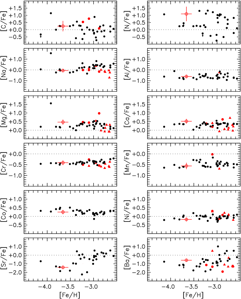
Figure 5: Relative abundances, [X/Fe], as a function of [Fe/H]. Boo$-$1137 is represented by an open red circle, while filled red circles stand for giants in the ultra-faint dSph Com Ber and U Ma II (Frebel et al. 2009) and the filled red triangles for stars in the more luminous Sextans dSph (Aoki et al. 2009). The filled black circles are from Cayrel et al. (2004) (Na–Ni), Spite et al. (2005) (C and N), and François et al. (2007) (Sr and Ba), respectively.

Figure 5 presents [X/Fe] as a function of [Fe/H], in the range –4.5 $<$ [Fe/H] $<$ –2.55, for 12 representative elements in Boo$-$1137 (the open red circle) and some $\sim$ 30 metal-poor Galactic red giants having high-resolution, high $S/N$, abundance analyses, together with data for dSph systems known to have member stars in the range [Fe/H] $\lesssim$ –3.1. For the halo stars, for reasons of homogeneity, we restrict the data to the results of the First Stars consortium (Cayrel et al. 2004; Spite et al. 2005; and François et al. 2007), while for the ultra-faint dSph we plot the results of Frebel et al. (2009; Com Ber and U Ma II, filled red circles) and for the more luminous Sextans dSph the data of Aoki et al. (2009) (filled red triangles).

It is important to recall that all of the data in the figure have been determined using 1D model atmospheres and the LTE approximation. This should be borne in mind when comparison is made with predictions of stellar evolution and galactic chemical enrichment models. For an appreciation of modifications that need to be made to the present abundances to take into account the role of more realistic 3D models and non-LTE effects we refer the reader to Asplund (2005), and references therein. That said, the question we are interested to address here is the similarity or otherwise between the most metal-poor dSph stars and those of the Galactic halo. Insofar as we have established that our 1D, LTE techniques reproduce the abundances of Cayrel et al. (see §3), Figure 5 suffices for our needs.

As one moves from top to bottom in Figure 5, six pairs of related elements are plotted – representing the CNO group, the light odd-Z elements, the $\alpha$-elements, the Fe-peak below (Cr and Mn) and above (Co and Ni) iron, and the neutron-capture elements. Initial inspection of the figure suggests an overall similarity between the relative abundances of Boo$-$1137 and those of the Galactic halo at [Fe/H] $\sim$ –3.5. We make the following points: (1) For [C/Fe] and [N/Fe], given the large dispersion in the measured field star abundance ratios, and our large observational errors, the results for Boo-1137 are consistent with those for the Galactic halo ; (2) For [Cr/Fe], [Mn/Fe], [Co/Fe], and [Ni/Fe] (the Fe-peak elements for which we have data) the 1$\sigma$ error bars all overlap the Cayrel et al. (2004) regression lines (their Table 9), supporting the view that similar processes and enrichment occurred for the material from which Boo$-$1137 and the Galactic halo formed. It also suggests that the present techniques produce results on the same system as those of Cayrel et al. (2004), strengthening the similar conclusion reached in §3.2, based on our analysis of the Cayrel et al. data; (3) For the light odd-Z elements, the Boo$-$1137 [Na/Fe] and [Al/Fe] data overlap those of the halo at the 1$\sigma$ level; (4) Of the two heavy neutron-capture elements, [Sr/Fe] lies within the values for halo stars, while [Ba/Fe] appears high. Given the complicated trend and scatter in [Ba/Fe] values seen in the figure, and the paucity of stars below [Fe/H] = –3.5, more data would be required to address this issue; and (5) For the representative $\alpha$-elements, the [Mg/Fe] and [Ca/Fe] values of Boo$-$1137 are both higher, by approximately twice their errors of measurement, than the Cayrel et al. (2004) regression lines of the Galactic halo.

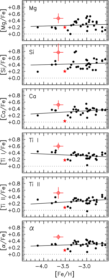
Figure 6: Relative abundances [X/Fe] for the $\alpha$-elements as a function of [Fe/H], where we use [$\alpha$/Fe] to denote the average of the relative abundances of [Mg/Fe], [Ca/Fe], [Ti I/Fe], and [Ti II/Fe]. Boo$-$1137 is represented by an open red circle, while the filled black circles and the red star (for CS22968–014) are from Cayrel et al. (2004). See text for discussion.

Given that we also have abundances for the $\alpha$-elements Si and Ti, we examine the final point more closely in Figure 6, which shows results for [Mg/Fe], [Si/Fe], [Ca/Fe], and [Ti/Fe], together with [$\alpha$/Fe] (the average of [Mg/Fe], [Ca/Fe], and [Ti/Fe]) as a function of [Fe/H]. Also shown in Figure 6 are the regression lines of Cayrel et al. (2004, their Table 9), supplemented by our linear least squares fits for Ti I, Ti II, and [$\alpha$/Fe] (not given individually by Cayrel et al.). There are interesting similarities in the panels of Figure 6: the most obvious (and relevant for the present discussion) is that all of the Boo$-$1137 relative abundances are larger that those of the Galactic halo at the [Fe/H] value of Boo$-$1137. Is this significant? To address this problem we proceed as follows. Rows (1)–(6), columns (1)–(7), of Table 4 present the relevant input data: columns (1)–(3) contain the atomic species involved, the RMS scatter for material having [Fe/H] $<$ –3.0 about the regression lines in Figure 6 (from Cayrel et al. (2004) and the present work), and the resulting values of the relative abundances of the Galactic halo at [Fe/H]_Boo-1137 = –3.66. Columns (4)–(7) show for Boo$-$1137 its relative abundance and error, the distance it falls above the halo line, and that distance expressed in units of the star’s abundance error. We then use Monte Carlo analysis to address the following question: if one draws putative stars at random from a gaussian distribution for a Galactic halo having the abundance dispersions in column (2), and superimposes on that a random gaussian error corresponding to the observational errors of Boo$-$1137 in column (5), what fraction of the resulting abundances would be at least as large as the observed distance of Boo$-$1137 above the halo lines (presented in column (6)). The results are presented in the final column of Table 4. One sees in rows (1)–(6) that, taken individually, the probabilities of Boo$-$1137 lying above the Galactic halo values are in the range 0.03–0.14, broadly consistent with the results in column (7) of the table. The most stringent condition, as might be expected, comes from the average of the $\alpha$-elements in the sixth row: the likelihood of finding the observed enhancement of the averaged $\alpha$-elements is 0.017.

One might also ask the question : what is the probability of all of the Boo$-$1137 [Mg/Fe], [Si/Fe], [Ca/Fe], [Ti I/Fe], and [Ti II/Fe] values falling above their respective Galactic halo lines. The answer, based on the Monte Carlo simulations, is that the fraction of relative abundances as large as seen for the five $\alpha$ species is 3 $\times$ 10^-6. This assumes, however, that the abundances of each of the above species is independent of all of the others, which is not the case, given the observed propensity of several of them to often have correlated behaviour. An example of such correlation is highlighted in Figure 6 where the red star represents the data of Cayrel et al. (2004) for CS22968–014, which for all species fall below the least-squares lines of best fit to the Cayrel et al. data. Had we performed the same test for CS22968–014 we would have concluded that the likelihood of all of the five species lying so far below the regression lines is 2 $\times$ 10^-4. (We note for completeness that McWilliam et al. (1995) also analyzed CS22968–014, and first reported the low relative abundances of its $\alpha$-elements.) The reader will see other examples of this effect in Figure 6. Given such correlated behavior, we shall not consider further the test in this paragraph, which is inappropriate.

The reader may recall from §3.2 that we found small systematic differences between the relative abundances of Cayrel et al. (2004) and those we obtained using our techniques. Those relevant here are $\Delta$[Mg I/Fe] = –0.049, $\Delta$[Ca I/Fe] = –0.008, $\Delta$[Ti I/Fe] = 0.033, and $\Delta$[Ti II/Fe] = –0.019, in the sense [Cayrel et al. – present work]. If we adjust the results in column (4) for these four species and [$\alpha$/Fe] to take the corrections into account, the fraction of Monte Carlo simulations having [$\alpha$/Fe] lying at or above the observed Boo$-$1137 values then increases to 0.024.

The above considerations depend on a knowledge of the dispersions in relative abundance in the Galactic halo. In the range –4.1 $<$ [Fe/H] $<$ –3.1, Cayrel et al. (2004) report dispersions for [Mg/Fe], [Si/Fe], [Ca/Fe], and [Ti/Fe] about their regressions against [Fe/H] of 0.11, 0.20, 0.11, and 0.09 dex, respectively. Inspection of Figure 6 suggests that given the decreasing sample size as one moves to lower abundances one should proceed with caution. For example, there are only five objects in the figure that have [Fe/H] $<$ –3.5. More data are clearly needed before one regard these estimates as definitive.

With this caveat in mind, we note that these dispersions for [Fe/H] $<$ –3.1 are somewhat larger than reported for metal-poor dwarfs in the range –3.0 $\lesssim$ [Fe/H] $\lesssim$ –2.0: by Magain (1989) – “extremely small (if any)”, by Nissen et al. (1994) – $\sigma$[Mg/Fe] = 0.06 dex, and by Arnone et al. (2005) – $\sigma$[Mg/Fe] = 0.06 dex. As discussed by these authors, and also by Argast et al. (2002), the dispersion of these elements at lowest abundance places strong constraints on the yields of SNe, the IMF, and galactic chemical enrichment at the earliest times. We shall return to the implications of this point below.

We note in concluding this section that Feltzing et al. (2009) have recently reported an anomalously large value of [Mg/Ca] = 0.73 (at [Fe/H] = –2.0) for one of seven stars they have observed in Boötes I (all with [Fe/H] $>$ –3.0). The value we obtain for Boo$-$1137 is [Mg/Ca] = –0.05, which is not too dissimilar from the mean value of 0.11 $\pm$ 0.06 that one obtains for their other six stars.

4.3 The Evolution and Chemical Enrichment of Boötes I

What are the implications from Figures 5 and 6 for the manner in which chemical enrichment occurred in Boötes I? As noted in §4.2 above, the initial impression of overall similarity between the abundances of Boo$-$1137 and those of the Galactic halo in Figure 5 is perhaps not too surprising. Intuitively, one might expect that for abundances as low as [Fe/H] = –3.7, and an old stellar population, it is more likely to find abundance patterns driven by enrichment from core-collapse supernovae from massive-star progenitors, without the later modification by Type SN Ia. This of course will depend on the rate and duration of star formation – only the earliest stars will have enrichment from only core-collapse supernovae, and, should galactic chemical enrichment occur for long enough, one will see the SN Ia signature downturn of [$\alpha$/Fe] vs [Fe/H] to more solar-like values as one moves from lower to higher [Fe/H]. In the Sculptor and Draco dSph, for example, the onset of the decrease is evident already at [Fe/H] $\sim$ –2.0, compared with –1.0 for the Galactic halo (see e.g. Tolstoy et al. 2009, their Figure 11, and Cohen & Huang 2009, respectively).

The chemical evolution of Boötes I probably involved a relatively short-lived epoch of star formation and self-enrichment in a dark matter dominated potential, terminated by catastrophic gas loss in (Type II)-supernova-driven winds (Saito 1979; Wyse & Silk 1985; Dekel & Silk 1986) in which the bulk of the initial (gaseous) baryonic mass was lost. As noted earlier, the color-magnitude diagram of Boötes I (Belokurov et al. 2006) is consistent with an old, metal-poor population. Forming stars would then have been chemically enriched by only core-collapse supernovae, resulting, for example, in enhanced [O/Fe] and [$\alpha$/Fe] compared with the solar value. The actual value of the relative enhancement depends on the mix of masses of the SNe progenitors, since model SNe yields show that more massive progenitors produce relatively more intermediate-mass elements than iron for many elements, so that an IMF biased towards the most massive stars will, with good sampling of the IMF and good mixing so that an IMF-average is achieved in star-forming regions, provide higher mean [O/Fe], [$\alpha$/Fe], etc. (see e.g. Wyse & Gilmore 1992; Argast et al. 2002; Kobayashi et al. 2006). The low stellar-mass and low level of enrichment of Boötes I mean that it would not be surprising if either the underlying IMF were not well-sampled in star-forming regions, or that they were not well-mixed, or both.

Our demonstration that the $\alpha$-elements appear enhanced with respect to iron in Boo-1137, relative to the mean of the metal-poor halo stars, by $\Delta[\alpha$/Fe] $\sim$ 0.2 is consistent with enrichment of the material from which Boo$-$1137 formed being biased towards the ejecta of SNe with more massive progenitors than the bulk of the metal-poor Galactic halo. This could reflect a biased underlying galaxy-scale IMF, or incomplete mixing and/or poor sampling of an invariant IMF, or be due to the shorter lifetimes of the most massive core-collapse progenitors in an invariant IMF.

We also know that Boötes I exhibits a large range in heavy element abundance – from samples of 16 and seven members of Boötes I Norris et al. (2008) and Feltzing et al. (2009) report ranges of 1.7 and 0.9 dex, respectively. Assuming a normal underlying galaxy-scale mass function, for which the stellar mass at $\sim 10$ Gyr after star formation burst is $\sim 50$% of the stars formed, and for which there is one $\sim 10$ M_⊙ SN progenitor for every $\sim 100$ M_⊙ of stars formed, and one 25 M_⊙ SN progenitor for every $\sim 1000$ M_⊙ formed, we can envisage that the early evolution of Boötes I formed $\sim 10^{5}~{}$M_⊙ in stars and $\sim 200$ Type II supernovae. Nissen et al. (1994) argued that the small dispersion, $\sigma$[Mg/Fe] = 0.06, they obtained for the Galactic halo is consistent with evolution in a well-mixed region with enrichment from some 25 SNe in the mass range 13–40 M_⊙ in a “preceding generation of totally about 2 $\times$ 10⁴ stars”. (From their Table 8, one would infer that the number of stars would be smaller by a factor of a few for the somewhat larger dispersions reported by Cayrel et al. (2004) and discussed above.). Given the resultant small number of cells this would imply if applied to Boötes I, it is not difficult to envisage incomplete mixing and poor sampling of the IMF across Boötes I, to give the apparent higher values of [$\alpha$/Fe] in Boo$-$1137. This is the most conservative of the three suggested reasons behind the elemental ratio enhancements we gave above, and we advocate this conclusion. Individual star-forming regions may well be internally mixed, while still poorly sampling the core-collapse supernovae IMF. A prediction of this would be that as more data are collected, one will observe the signature of a small number of internally well-mixed cells having preferred abundances.

There remains the objection that these conclusions are based on results for just one star. Statistical chance in selecting one star from a possibly diverse parent population, or in enriching one new star from an inhomogeneous star forming region, may undermine our conclusions. The analyses of larger samples of extremely metal-poor stars in Boötes I and in other dSph are awaited with much anticipation.

Table 1: AVERAGED EQUIVALENT WIDTHS, UPPER LIMITS, AND LINE-BY-LINE ABUNDANCES OF BOO–1137

	$\lambda$	$\chi$	$\log gf$	$W_{\lambda}$	$\log\epsilon$
Species	(Å)	(eV)	(dex)	(mÅ)	(dex)
(1)	(2)	(3)	(4)	(5)	(6)
Na I	5889.951	0.00	0.11	93.9	2.42
	5895.924	0.00	$-$0.19	77.8	2.48
Mg I	3829.355	2.71	$-$0.21	115.7	4.03
	3832.304	2.71	0.15	153.1	4.42
	3838.290	2.72	0.41	152.1	4.15
	4351.906	4.34	$-$0.52	44.6	4.89
	4702.991	4.35	$-$0.67	23.4	4.64
	5172.684	2.71	$-$0.38	130.2	4.17
	5183.604	2.72	$-$0.16	142.1	4.19
	5528.405	4.34	$-$0.34	22.2	4.24
Al I	3944.006	0.00	$-$0.64	79.4	2.18
	3961.520	0.01	$-$0.34	86.2	2.01
Si I	3905.523	1.91	$-$1.09	147.6	4.62
Ca I	4226.728	0.00	0.24	135.6	2.74
	4283.011	1.89	$-$0.22	22.8	3.17
	4454.779	1.90	0.26	52.5	3.24
	5588.749	2.52	0.21	12.7	3.11
	6102.723	1.88	$-$0.79	8.4	3.14
	6122.217	1.89	$-$0.32	24.1	3.21
	6162.173	1.90	$-$0.09	33.1	3.17
	6439.075	2.52	0.47	19.2	3.03
	6493.781	2.52	$-$0.11	22.5	3.69
Sc II	4246.822	0.31	0.24	74.1	$-$0.93
	4314.083	0.62	$-$0.10	35.3	$-$0.78
	4400.389	0.61	$-$0.54	22.9	$-$0.59
Ti I	3998.636	0.05	$-$0.06	48.5	1.88
	4981.731	0.84	0.50	27.4	1.80
	4991.065	0.84	0.38	21.5	1.79
	4999.503	0.83	0.25	22.7	1.93
	5210.385	0.05	$-$0.88	12.4	1.81
Ti II	3759.296	0.61	0.27	141.2	1.55
	3761.323	0.57	0.17	156.3	1.89
	3913.468	1.12	$-$0.41	100.6	1.78
	4012.385	0.57	$-$1.75	73.3	1.85
	4290.219	1.16	$-$0.93	68.8	1.62
	4300.049	1.18	$-$0.49	82.2	1.44
	4394.051	1.22	$-$1.77	29.5	1.87
	4395.033	1.08	$-$0.51	98.2	1.63
	4399.772	1.24	$-$1.22	57.3	1.81
	4418.330	1.24	$-$1.99	23.1	1.98
	4443.794	1.08	$-$0.70	92.6	1.70
	4444.558	1.12	$-$2.21	19.0	1.95
	4450.482	1.08	$-$1.51	56.8	1.89
	4464.450	1.16	$-$1.81	43.0	2.07
	4468.507	1.13	$-$0.60	96.8	1.74
	4501.273	1.12	$-$0.76	80.6	1.56
	5188.680	1.58	$-$1.05	42.0	1.74
	5226.543	1.57	$-$1.23	29.2	1.68
	5336.771	1.58	$-$1.63	14.4	1.71
Cr I	4254.332	0.00	$-$0.11	69.3	1.37
	4274.796	0.00	$-$0.23	58.4	1.31
	4289.716	0.00	$-$0.36	56.0	1.40
	5206.038	0.94	0.02	37.2	1.76
	5208.419	0.94	0.16	43.1	1.72
	5409.772	1.03	$-$0.72	9.5	1.87
Mn I	4030.753	0.00	$-$0.48	60.2	1.17
	4033.062	0.00	$-$0.62	46.3	1.15
	4034.483	0.00	$-$0.81	35.3	1.19
Fe I	3763.789	0.99	$-$0.24	129.6	3.70
	3767.192	1.01	$-$0.39	110.6	3.40
	3786.677	1.01	$-$2.23	45.0	3.80
	3787.880	1.01	$-$0.86	107.3	3.77
	3815.840	1.48	0.24	125.2	3.67
	3820.425	0.86	0.12	158.0	3.70
	3824.444	0.00	$-$1.36	150.2	4.05
	3825.881	0.91	$-$0.04	136.8	3.54
	3827.823	1.56	0.06	103.2	3.38
	3840.438	0.99	$-$0.51	120.4	3.71
	3849.967	1.01	$-$0.97	122.2	4.24
	3856.372	0.05	$-$1.29	142.2	3.87
	3859.911	0.00	$-$0.71	167.4	3.66
	3865.523	1.01	$-$0.98	116.8	4.10
	3878.018	0.96	$-$0.91	111.6	3.83
	3886.282	0.05	$-$1.08	152.0	3.84
	3887.048	0.91	$-$1.14	102.7	3.77
	3895.656	0.11	$-$1.67	132.3	4.09
	3899.707	0.09	$-$1.53	137.2	4.04
	3920.258	0.12	$-$1.75	129.2	4.10
	3922.912	0.05	$-$1.65	131.8	3.97
	4005.242	1.56	$-$0.61	94.4	3.77
	4045.812	1.48	0.28	133.8	3.72
	4063.594	1.56	0.07	110.2	3.46
	4071.738	1.61	$-$0.02	118.4	3.81
	4132.058	1.61	$-$0.67	79.4	3.52
	4143.868	1.56	$-$0.46	105.4	3.84
	4187.039	2.45	$-$0.55	34.5	3.61
	4187.795	2.42	$-$0.55	45.2	3.76
	4191.431	2.47	$-$0.73	35.5	3.83
	4199.095	3.05	0.25	31.5	3.46
	4202.029	1.48	$-$0.70	84.5	3.48
	4222.213	2.45	$-$0.97	26.7	3.87
	4233.603	2.48	$-$0.60	25.2	3.50
	4250.119	2.47	$-$0.40	48.1	3.71
	4260.474	2.40	$-$0.02	68.8	3.60
	4271.154	2.45	$-$0.35	45.7	3.59
	4271.761	1.48	$-$0.16	107.9	3.46
	4282.403	2.17	$-$0.82	36.4	3.57
	4337.046	1.56	$-$1.70	52.0	3.98
	4383.545	1.48	0.20	125.7	3.49
	4404.750	1.56	$-$0.14	113.2	3.62
	4415.123	1.61	$-$0.61	101.2	3.87
	4447.717	2.22	$-$1.34	27.2	3.96
	4461.653	0.09	$-$3.20	85.4	4.26
	4494.563	2.20	$-$1.14	31.9	3.83
	4871.318	2.87	$-$0.36	27.0	3.71
	4872.138	2.88	$-$0.57	21.1	3.80
	4891.492	2.85	$-$0.11	33.8	3.57
	4918.994	2.87	$-$0.34	21.1	3.56
	4920.503	2.83	0.07	45.9	3.57
	4939.687	0.86	$-$3.34	10.6	3.81
	4994.130	0.92	$-$3.08	19.5	3.92
	5041.072	0.96	$-$3.09	27.5	4.16
	5049.820	2.28	$-$1.36	16.9	3.75
	5083.339	0.96	$-$2.96	21.4	3.89
	5123.720	1.01	$-$3.07	21.8	4.07
	5150.840	0.99	$-$3.04	16.8	3.88
	5151.911	1.01	$-$3.32	12.5	4.03
	5166.282	0.00	$-$4.20	27.9	4.10
	5171.596	1.49	$-$1.79	49.2	3.86
	5192.344	3.00	$-$0.42	16.3	3.64
	5194.942	1.56	$-$2.09	33.7	3.99
	5216.274	1.61	$-$2.15	21.5	3.85
	5232.940	2.94	$-$0.06	29.1	3.52
	5266.555	3.00	$-$0.39	16.8	3.62
	5269.537	0.86	$-$1.32	121.8	3.94
	5324.179	3.21	$-$0.24	16.8	3.72
	5328.039	0.92	$-$1.47	108.7	3.86
	5328.532	1.56	$-$1.85	32.3	3.72
	5371.490	0.96	$-$1.65	107.6	4.05
	5397.128	0.92	$-$1.99	85.2	3.92
	5405.775	0.99	$-$1.84	88.4	3.91
	5429.697	0.96	$-$1.88	88.8	3.91
	5434.524	1.01	$-$2.12	71.2	3.92
	5446.917	0.99	$-$1.91	89.5	3.99
	5455.609	1.01	$-$2.09	71.6	3.90
	5497.516	1.01	$-$2.85	24.2	3.88
	5506.779	0.99	$-$2.80	32.7	3.97
	5586.756	3.37	$-$0.14	13.1	3.66
	6393.601	2.43	$-$1.58	11.2	3.87
Fe II	4233.172	2.58	$-$1.90	35.3	3.66
	4923.927	2.89	$-$1.50	47.7	3.79
Co I	3845.461	0.92	0.01	59.5	1.50
	3995.302	0.92	$-$0.22	50.5	1.53
	4118.767	1.05	$-$0.49	23.1	1.52
	4121.311	0.92	$-$0.32	40.8	1.51
Ni I	3775.565	0.42	$-$1.39	68.2	2.37
	3807.138	0.42	$-$1.18	75.9	2.31
	3858.292	0.42	$-$0.97	93.8	2.51
	5476.900	1.83	$-$0.89	15.5	2.38
Sr II	4077.710	0.00	0.16	70.0	$-$2.15
	4215.520	0.00	$-$0.16	51.5	$-$2.17
Ba II	4934.076	0.00	$-$0.15	40.5	$-$2.20
	6141.730	0.70	$-$0.08	14.4	$-$2.09
	6496.910	0.60	$-$0.38	13.6	$-$1.96

Table 2: 1D LTE ABUNDANCES OF BOO–1137

Species	N${}_{\mbox{\scriptsize lines}}$	$\log\epsilon(\mbox{X})$	s.e.logϵ	[X/Fe]
(1)	(2)	(3)	(4)	(5)
C(CH)	syn	$4.98$	$0.20$	$0.25$
N(NH)	syn	$5.22$	$0.30$	$1.10$
O I	1	$<6.94$	$...$	$<1.94$
Na I	2	$2.45$	$0.05$	$-0.06$
Mg I	8	$4.34$	$0.10$	$0.47$
Al I	2	$2.10$	$0.11$	$-0.61$
Si I	1	$4.62$	$...$	$0.77$
Ca I	9	$3.17$	$0.08$	$0.52$
Sc II	3	$-0.77$	$0.12$	$-0.16$
Ti I	5	$1.84$	$0.04$	$0.60$
Ti II	19	$1.76$	$0.05$	$0.52$
Cr I	6	$1.57$	$0.10$	$-0.41$
Mn I	3	$1.17$	$0.02$	$-0.56$
Fe I	81	$3.79$	$0.02$	$-3.66\tablenotemark{c}$
Fe II	2	$3.73$	$0.08$	$-0.06$
Co I	4	$1.51$	$0.02$	$0.25$
Ni I	4	$2.39$	$0.05$	$-0.18$
Zn I	1	$<1.64$	$...$	$<0.70$
Sr II	2	$-2.16$	$0.02$	$-1.42$
Ba II	3	$-2.08$	$0.08$	$-0.59$
Eu II	1	$<-2.65$	$...$	$<0.49$

Table 3: ABUNDANCE ERRORS FROM UNCERTAINTIES IN ATMOSPHERIC PARAMETERS

Species	$\Delta$$T_{\rm eff}$	$\Delta$log $g$	$\Delta$[M/H]	$\Delta\xi_{t}$	$\Delta$[X/Fe]
	(200K)	(0.3 dex)	(0.3 dex)	(0.2 km s-1)	(dex )
(1)	(2)	(3)	(4)	(5)	(6)
C	$0.28$	$-0.08$	$0.00$	$0.00$	$0.29$
N	$0.38$	$-0.08$	$0.00$	$0.00$	$0.39$
Na I	$-0.02$	$0.00$	$0.00$	$-0.03$	$0.03$
Mg I	$-0.10$	$0.01$	$0.00$	$0.00$	$0.10$
Al I	$0.02$	$-0.01$	$0.00$	$-0.06$	$0.06$
Si I	$0.00$	$-0.07$	$-0.02$	$-0.14$	$0.16$
Ca I	$-0.10$	$0.00$	$0.00$	$-0.01$	$0.10$
Sc II	$-0.08$	$0.10$	$0.01$	$-0.01$	$0.13$
Ti I	$0.04$	$-0.01$	$-0.01$	$-0.01$	$0.04$
Ti II	$-0.12$	$0.11$	$0.01$	$0.00$	$0.16$
Cr I	$0.02$	$0.00$	$0.00$	$0.00$	$0.02$
Mn I	$0.08$	$-0.01$	$-0.01$	$-0.01$	$0.08$
Fe I	$0.11\tablenotemark{a}$	$-0.02\tablenotemark{a}$	$0.00\tablenotemark{a}$	$0.00\tablenotemark{a}$	$0.11\tablenotemark{a}$
Fe II	$-0.20$	$0.10$	$0.00$	$-0.02$	$0.22$
Co I	$0.06$	$0.00$	$0.00$	$-0.01$	$0.06$
Ni I	$0.02$	$0.00$	$0.00$	$0.00$	$0.02$
Sr II	$-0.06$	$0.10$	$0.01$	$-0.03$	$0.12$
Ba II	$-0.06$	$0.10$	$0.01$	$-0.01$	$0.12$

Table 4: MONTE-CARLO ANALYSIS OF BOO-1137 $\alpha$-ELEMENT RELATIVE ABUNDANCES

Species	RMSHalo	[X/Fe]Halo	[X/Fe]Boo	$\sigma$[X/Fe]Boo	$\Delta$[X/Fe]	$\Delta$[X/Fe]/	Fraction
						$\sigma$[X/Fe]Boo
(1)	(2)	(3)	(4)	(5)	(6)	(7)	(8)
Mg I	0.11	0.250	0.470	0.14	0.220	1.57	0.108
Si I	0.20	0.412	0.770	0.26	0.358	1.38	0.138
Ca I	0.11	0.290	0.520	0.13	0.230	1.77	0.089
Ti I	0.09	0.346	0.600	0.10	0.254	2.54	0.029
Ti II	0.11	0.234	0.520	0.17	0.286	1.68	0.079
$\alpha$	0.09	0.274	0.516	0.07	0.242	3.40	0.017