Phenomenological Implications of Supersymmetric Family Non-universal ModelsLisa L. Everetta, Jing Jianga, Paul G. Langackerb and Tao LiucaDepartment of Physics, University of Wisconsin,
Madison, WI 53706
bSchool of Natural Science, Institute for Advanced Study,
Einstein Drive, Princeton, NJ 08540
cEnrico Fermi Institute,
University of Chicago,
5640 S. Ellis Ave., Chicago, IL
60637
Abstract
We construct a class of anomaly-free supersymmetric models that are characterized by family non-universal charges motivated from embeddings. The family non-universality arises from an interchange of the standard roles of the two representations within the of for the third generation. We analyze and electroweak symmetry breaking and present the particle mass spectrum. The models, which include additional Higgs multiplets and exotic quarks at the TeV scale, result in specific patterns of flavor-changing neutral currents in the transitions that can accommodate the presently observed deviations in this sector from the SM predictions.
1 Introduction
Extensions of the Standard Model of particle physics (SM) with an additional anomaly-free gauged symmetry broken at the TeV scale are arguably some of the most well-motivated candidates for new physics (for a review, see [1]). Such symmetries are theoretically motivated, as they represent the simplest augmentations of the SM gauge sector and are ubiquitous within string and/or grand unified theories. While the phenomenology of such gauge bosons depends on the details of the couplings of the to the SM fermions, current limits from direct and indirect searches indicate typical lower bounds of order GeV on the mass and an upper bound of on the mixing angle [2]. For a reasonable range of couplings, the presence of such TeV scale bosons should be easily discernable at present and forthcoming colliders such as the Tevatron and the Large Hadron Collider (LHC).
Within the context of supersymmetric theories, a plethora of models have been proposed, including scenarios motivated by grand unified theories (GUTs) such as and and scenarios motivated from string compactifications of heterotic and/or Type II theories (see [1] for a review). Recent models also include scenarios in which the mediates supersymmetry breaking [3], plays a role in the generation of neutrino masses [4] and/or spontaneous -parity violation [5], or provides a portal to a hidden/secluded sector (for reviews, see [6, 7]). Though the details of the charge assignments are model-dependent, generically the cancellation of anomalies requires an enlargement of the matter content to include SM exotics and SM singlets with nontrivial charges. In these theories, the SM singlets also typically play an important role in triggering the low-scale breaking of the gauge symmetry.
In most models of this type, the charges of the quarks and leptons are family universal. Though this feature is desirable for the first and second generations due to the strong constraints from flavor-changing neutral currents (FCNCs), there is still room for departures from family universality for the charges of the third generation. In fact, this often occurs in string constructions if the families result from different embeddings (see e.g., [8, 9]). Indeed, though many of the results from the factories have indicated a strong degree of consistency with the Cabibbo-Kobayashi-Maskawa (CKM) predictions of the SM, there are hints of non-SM FCNC patterns within the transitions for both and processes at the level of a few standard deviations [10].
Of the many options for new physics models that can explain this discrepancy, family non-universal models are interesting in that they are theoretically well-motivated scenarios that lead to tree-level FCNC, as opposed to scenarios in which the new physics contributions are loop-suppressed [11]. A recent model-independent analysis of -mediated FCNC in the transitions showed that this general framework can accommodate the data [12, 13]. (Related analyses include [14, 15]). However, it is optimal to consider the bounds on specific family non-universal models in addition to the fully model-independent results.
Our purpose in this paper is to construct and analyze supersymmetric anomaly-free family non-universal models (which we will denote as NUSSM models). Our strategy in building this class of NUSSM models is to exploit the well-known fact that in models, there are two options for embedding the down quarks and lepton doublets in the representation of , which is related to the fact that the down-type Higgs and the lepton doublets have the same gauge quantum numbers. By choosing one embedding for the first and second generations and the alternative embedding for the third generation, we can obtain anomaly-free models in which the additional family non-universal is given by a particular linear combination of the usual and of -inspired models.
This paper is structured as follows. We begin by outlining our basic procedure and presenting the resulting classes of anomaly-free family non-universal models. In the following section, we analyze the gauge symmetry breaking and comment on general features of the mass spectrum. We next turn to an analysis of the implications of these models for FCNC in the transitions, then provide our concluding remarks.
2 -Motivated Family Non-universal Models (NUSSMs)
Table 1: The decomposition of the fundamental
representation of with respect to the , , and subgroups. and correspond to specific linear combinations of the and gauge groups that result from and , respectively.
(1st and 2nd families)
(3rd family)
16
1
0
3
1
1
27
10
2
0
1
0
4
In models, the cancellation of gauge anomalies generally implies that additional fermions are present in the theory (see e.g., [1]). To motivate the presence of these additional fermions and construct simple anomaly-free family non-universal models, our approach is to exploit the properties of embeddings of the SM fermions and Higgs fields in grand unified theories. Recall that in models, the SM particles are embedded in the fundamental representations. With respect to the two-step breaking scheme of to its and subgroups
(2.1)
the has the decomposition
(2.2)
with respect to the representations of and , respectively. Hence, the has two multiplets; these representations are used to embed the down-type -singlet quarks with the lepton doublets and exotic -singlet quarks with down-type Higgs doublets. A standard choice for model-building is to have the down-type quarks and lepton doublets of all three SM families in the of the , though models with the SM down-type quarks and lepton doublets in the other have also been considered in the literature [16, 17].
We will assign the down-type quark singlets and lepton doublets of the first and second generations to be in the of the , and the associated particles of the third generation to be in the of the , as shown in Table 1. The matter content of these theories thus includes the following fields: (i) the SM first and second families , Higgs plus exotic fields , and singlets ( is a family index), and (ii) the SM third family , Higgs and exotics , and singlet . The Higgs sector of the theory thus generically has multiple Higgs doublets and singlets beyond those of the MSSM.111MSSM-type gauge unification requires the introduction of an additional non-chiral Higgs pair from an incomplete [18].
The additional family non-universal in these NUSSM models is then a linear combination of the and the gauge groups:
(2.3)
(the assumption is that the orthogonal linear combination of and is either absent or broken at a high scale).
The familiar group, which has , is family universal and therefore is not useful for our purposes.222This linear combination occurs in certain Calabi-Yau compactifications of heterotic string theory if breaks to a rank 5 group via the Hosotani mechanism [19]. Two viable options for the additional group are:
•
(). In this model (the inert model) the gauge boson couplings to the up-type quarks vanish [20] . Hence, the production of the associated boson is suppressed at hadron colliders. This is especially the case at the Tevatron, since in high-energy collisions the production via down quarks is suppressed by an order of magnitude relative to up quarks [21].
•
(). This symmetry is motivated by models with a secluded breaking sector and a large supersymmetry breaking -term that have (1) an approximately flat potential that results in an appropriate – mass hierarchy [22]; (2) a strong first order electroweak phase transition and large spontaneous CP-violation, which can result in viable electroweak baryogenesis [23].
While we use the framework to motivate the matter content and charges of these models, we do not work within a full grand unified theory. More precisely, we do not impose the Yukawa coupling relations. This allows for a TeV-scale without the danger of rapid proton decay.333Detailed studies of theories with broken Yukawa relations can be found in [17].
The allowed superpotential terms of NUSSM models (assuming a conserved -parity) are the couplings that are consistent with the SM and gauge symmetries. An inspection of Table 1 shows that in the language of the decomposition, the usual and terms that give rise to quark and lepton Yukawa couplings for all three families (including mixing terms between the third family and the other two families) are allowed by both and . Similarly, these symmetries allow the generation of Yukawa interactions for the exotic quarks and for the Higgs doublets with the SM singlets (i.e., mass terms for the exotic quarks and effective terms for the Higgs fields, which will be of importance for gauge symmetry breaking).
For simplicity, we assume that only the neutral Higgs bosons from the third family ( and ) and one of the first two families ( and ) acquire vacuum expectation values (VEVs).444This is actually without loss of generality by appropriate field redefinitions.
In this limit, the Higgs bosons and Higgsinos in the other family have no mixing at leading order with
the other particles. The mass eigenvalues of these particles are determined by the VEVs of
as well as the Yukawa couplings and soft parameters which are not directly involved in the electroweak symmetry breaking.
In this article, therefore, we will not discuss them in detail. The relevant superpotential terms are then given by ( and are family indices):
(2.4)
(2.5)
in which the Yukawa couplings satisfy the relations , ,
, , , and . In Eq. (2.5), represents additional superpotential terms that are consistent with or , but explicitly break the orthogonal linear combination of and . These terms are needed to avoid the appearance of undesirable light axions in the low energy theory (see [24] for a recent discussion).
For the model, is a bilinear term:
(2.6)
Although the coupling in is dimensionful, there is no associated problem in the traditional sense. This term is not necessary for or electroweak symmetry breaking, so its mass scale need not be connected with the electroweak scale. The Giudice-Masiero mechanism [25] therefore can be implemented in both gravity- and gauge-mediated breaking frameworks to produce such a term, even though the in the latter case is typically small. In the model, consists of the trilinear term
(2.7)
In what follows, we will focus on the model as a concrete and minimal example, and defer the model for future study.
3 Particle Mass Spectrum and Gauge Symmetry Breaking
The gauge group of the NUSSM model is given by , with gauge couplings , , , and , respectively. The matter content, which was presented in Table 1, includes three sets of Higgs fields (one pair of doublets and one singlet per family) and three sets of exotic down-type quarks in addition to the MSSM fields. As previously discussed, we assume that only two of the three Higgs doublet pairs ( and ) acquire vacuum expectation values, and hence focus on the couplings of these Higgs fields only. Restricting to this set of terms, the superpotential for the model is given in Eq. (2.4), Eq. (2.5), and Eq. (2.6).
The tree-level Higgs potential (for the neutral components of the fields) is given by , in which
(3.8)
(3.10)
where . We also include the one-loop contribution to the potential:
(3.11)
in which denotes the field-dependent mass-squared matrices of the theory,
and is the
renormalization scale. We will only consider the dominant one-loop contributions that arise from the top quark sector:
(3.12)
The Higgs potential allows for a rich structure of CP-violating effects, including explicit CP violation (for complex couplings) and spontaneous CP violation. In this work, we will assume that all couplings are real and let the potential parameters satisfy some necessary constraints such that spontaneous CP violation can be avoided. In this case, the vacuum expectation values of the neutral Higgs components can be taken to be real:
(3.13)
Before turning to a numerical analysis, we begin with a general discussion of the particle mass spectrum, starting with the gauge bosons.
The mass-squared matrix is
(3.14)
in which
(3.15)
with . The mass-squared eigenvalues are
(3.16)
and the mixing angle is
(3.17)
which is bounded to be less than a few times (see [2] for a recent discussion).
This typically requires that the singlet vacuum expectation values TeV, resulting in a TeV-scale mass. The charged gauge boson mass is given as usual by
.
In the basis , the neutralino mass matrix is
(3.18)
in which
(3.19)
In the above, , and , , and are the gaugino mass parameters for
, , and , respectively.
The chargino mass matrix is
(3.20)
Since because of the experimental bounds on , the charginos and neutralinos are typically heavy unless the ’s are small or the gaugino masses are light. In the latter situation, the lightest chargino and neutralino will be gaugino-like.
The mass-squared matrices of the sfermions (denoted collectively as ) are
(3.21)
With the definitions
(3.22)
(3.23)
the entries for example of the up-type squark mass-squared matrix are:
(3.24)
Analogous expressions can be written for the down-type squarks, sleptons, and sneutrinos.
The physical Higgs spectrum consists of 6 CP-even neutral Higgs bosons, 4 CP-odd neutral Higgs bosons, and 6 charged Higgs bosons (not including the second family). The tree-level charged Higgs boson mass-squared matrix is given in the Appendix.
Next we turn to a numerical analysis of this sector of the model, taking into account the constraints on the gauge boson.
We explore the viable regions of parameter space in which (i) , which is needed for a TeV scale , and (ii) , which is motivated by the observed hierarchies in the SM fermion mass spectrum. To obtain an acceptable minimum, typically we need the Higgs soft mass parameters to satisfy or . We also set the gauge coupling to and enforce the following constraints on the Yukawa couplings:555This approximation must be relaxed slightly to obtain CKM mixing of the third family with the first and second families, but that is irrelevant for our present purposes.
(3.25)
which result in the condition
(3.26)
in which we have included the one-loop QCD corrections to the top quark mass.
We consider one typical numerical example; the relevant input parameters and results are summarized in Tables 2–4. The mass spectrum of the neutral Higgs bosons are calculated at one-loop level, and the mass spectra of the other particles are calculated at tree-level. As a check, we estimate the mass and the mixing angle by using the Higgs VEVs given in Table 2, as follows:
(3.27)
which is consistent with the detailed results. The lightest CP-even Higgs boson is a linear combination of the real parts of the four Higgs doublets, with a negligible singlet admixture; the orthogonal linear combinations of these four states are the , , and bosons. These heavier Higgs bosons fall into multiplets together with the three heaviest CP-odd states and the set of charged Higgs bosons, as follows: , , and . The second lightest and second heaviest CP-even states are admixtures of the two singlet Higgs fields, as is the lightest CP-odd boson (which has a mass that controlled by the Higgs bilinear terms). The chargino and neutralino mass spectrum is highly model-dependent, as it is sensitive to the electroweak and hypercharge gaugino masses, which do not strongly impact the gauge symmetry breaking. Hence, the physics of the lightest superparticle (LSP) can vary greatly depending on the exact structure of the gaugino sector, though the gauge and Higgs sectors can remain almost the same in this case. In our numerical example, in which the gaugino masses are light and obey GUT relations, the LSP is a predominantly bino-like neutralino that can be an acceptable dark matter candidate in regions of the parameter space.666The neutralino sector has additional complications due to the presence of the additional Higgs supermultiplets that do not participate in electroweak symmetry breaking at tree level. Hence, a detailed numerical analysis would be needed to ascertain whether the neutralino LSP satisfies the dark matter constraints. As this is tangential to the main purpose of our paper, we do not address it here.
Finally, we comment on the exotic colored particles and . The exotic scalars do not
obtain VEVs. They and their superpartners influence the gauge symmetry breaking only at loop level. These exotic particles are chiral, so their tree-level masses can be produced only through Yukawa interactions. The superpotential terms that describe their interactions with the Higgs fields and the corresponding soft supersymmetry breaking terms are
(3.28)
(3.29)
It is straightforward to determine the mass matrices for these states for given Yukawa couplings and parameter values. For (where their contributions to the effective neutral Higgs potential can be neglected)
and not large values, the exotic particles will typically obtain masses of the order of several hundred GeV.
Table 2: Parameter values and Higgs VEVs. The dimensional parameter values are given in GeV or GeV2. The Higgs VEVs are given in GeV.
0.10
0.30
0.10
449
0.60
112
112
224
673
1080
897
54.8
83.7
2000
93.3
108
4010
Table 3: The particle mass spectrum and mixing angle of the NUSSM model (all masses are in GeV).
/
1900
275
609
219
114
/
/
173
369
1100
1640
1970
2360
/
633
1080
1650
2340
1060
1630
2330
Table 4: The composition of the neutral Higgs mass eigenstates at the one-loop level.
0.31
0.48
-0.09
0.53
0.61
-0.07
0.07
0.06
0.87
0.06
0.05
0.49
-0.28
0.86
-0.02
-0.34
-0.25
0.03
-0.88
-0.11
0.02
0.13
0.43
0.04
0.03
-0.01
-0.49
0.04
-0.01
0.87
-0.20
0.06
0.01
0.76
-0.61
-0.03
-0.04
-0.02
0.89
-0.01
-0.01
0.45
0.26
0.87
0.03
0.35
-0.24
0.02
0.89
-0.10
0.04
-0.12
0.43
0.01
-0.20
-0.08
-0.01
0.76
0.62
0.02
0.30
-0.33
0.20
0.59
-0.52
-0.39
-0.12
0.21
-0.40
-0.25
0.26
0.81
Table 5: The composition of the charged Higgs mass eigenstates at tree level.
0.26
0.87
0.34
-0.23
0.89
-0.10
-0.12
0.42
-0.20
-0.07
0.75
0.62
0.31
-0.47
0.55
-0.62
4 -mediated FCNC Effects
In this section, we analyze the -induced FCNC effects After a brief review of the formalism, we will show the results of our correlated analysis of the processes via transitions and discuss the resulting parameter space constraints.
The processes of interest include mixing and the time-dependent CP asymmetries of the penguin-dominated neutral decays.
The FCNC effects in general NUSSM models include both -mediated FCNC processes and contributions to FCNC from the soft supersymmetry breaking parameters. In this work, we assume for simplicity that the soft terms do not result in large FCNC effects (this can be easily achieved;
see e.g. [26]) and consider only the contributions. We now briefly discuss the formalism for addressing such effects in the NUSSM (for a model-independent discussion, see [11, 12, 13]).
For the SM fermions with charges , the fermion mass matrices are diagonalized by the biunitary transformation
(the CKM matrix is
).
The chiral couplings in the fermion mass eigenstate basis are
(4.30)
In our model, the only SM fields with nontrivial charges are the down-type quark singlets and the lepton doublets:
(4.31)
With the unitary matrices written as
(4.32)
where is a submatrix, one obtains
(4.33)
To avoid the constraints on non-universality for the first two families from mixing and conversion in muonic atoms, we assume small fermion mixing angles or small , elements. The couplings then take the form
(4.34)
Here and generically are complex.
The -induced corrections to the Wilson coefficients in the model777In the model, in which all SM fermions are charged under the symmetry, the -induced corrections to the Wilson coefficients take a more general form (see e.g. [12, 13]). We will not discuss them here. are given by (for the associated operators, see e.g. [13]):
(4.35)
To achieve sufficient precision, we need to have an accurate knowledge of the relevant Wilson coefficients at the quark mass scale GeV (for general discussions, see e.g. [27]). The parameter values used in our calculations are summarized in Appendix B.
mixing. The new physics (NP) contributions to the off-diagonal mixing matrix element are parametrized as
(4.36)
where and in the SM limit. Although the data indicate that , a recent analysis [10] suggests that deviates from zero at the level (see Table 6); an earlier discussion was given in [28]. The analysis of [10] includes all available results on mixing, including the tagged analyses of by CDF [29] and D [30]. As discussed for example in [31], this discrepancy disfavors scenarios with minimal flavor violation (MFV), though no single measurement yet has a significance.
In our NUSSM model, and at the scale are given by
(4.37)
The large coefficients of the correction terms in Eq. (4.37) are due to the fact that the NP is introduced at tree-level while the SM limit is a loop-level effect.
Observable
C.L.
C.L.
(S1)
-20.3 5.3
[-30.5,-9.9]
(S2)
-68.0 4.8
[-77.8,-58.2]
1.00 0.20
[0.68,1.51]
Table 6: The fit results for the mixing parameters [10]. The two solutions (“S1” and “S2”) result from measurement ambiguities; see [10] for details.
decays.
(1 C.L.)
(1 C.L.)
Table 7: The world averages of the experimental results for the CP asymmetries in decays via transitions [32].
The direct and the mixing-induced CP asymmetries in hadronic decays are parametrized as follows:
(4.38)
in which
(4.39)
Here is the mixing angle, is the decay amplitude of ( is its CP conjugate), and
is the CP eigenvalue for the final state . In the SM, , and a non-trivial weak phase enters only at . This implies the following SM relation between the decays proceeding via and the penguin-dominated modes such as :
(4.40)
However, the experimental values of obtained from the penguin-dominated modes are below the SM prediction and the results from the charmed mode. The central values of the direct CP asymmetries of and are also small compared to the mode, as shown in Table 7. Since is a tree-level process in the SM, large values for and may indicate the presence of NP in the transitions.
In NUSSM models, -induced FCNC effects can provide dramatic changes to the results, since a new weak phase can enter at tree level. Following [33], the
parameters of at the scale are given by
These results are more general than those of [12, 13], as they include the contributions to both the QCD and electroweak penguins.
At the leading order, the deviations for and from their SM predictions are a linear combination of these two classes of contributions. This discussion is independent of the details of the charges, so it can be applied to
other family non-universal models as well; however, in the model, the only non-trivial corrections are and .
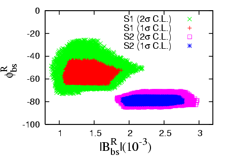
Figure 1: Correlated constraints on and . Random values for and from the experimentally allowed regions at different C.L. (see Table 1) are mapped to the plane using Eq. (4.37).
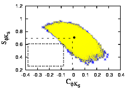
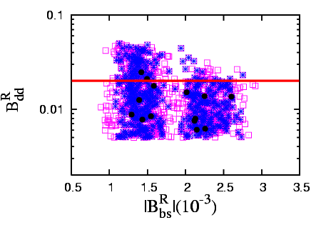
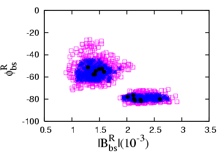
Figure 2:
The NP contributions to and , with , constrained by mixing. The colors specify the C.L. that their inverse image points represent in Fig. 1 (yellow for and blue for ). The boxes specify the allowed regions at 1 and , and the dark points denote the SM limit.
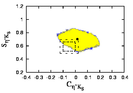
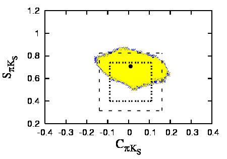
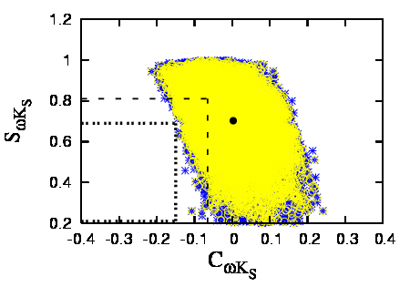
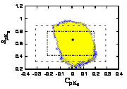
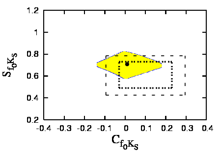
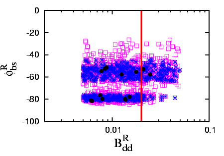
Figure 3: The , and distributions, with values constrained by mixing at C.L. and selected by and at C.L.. Here and for the purple points, and for the blue points, and for the dark points. The red lines represent the vacuum considered in Section 3, in which the values of and are not fixed.
We now turn to a numerical analysis of the FCNC constraints with the model, for which the three free parameters are , and . First, we consider mixing, which involves two of these parameters, and . The experimental constraints on these two parameters are illustrated in Fig. 1, where the various colors of the points specify the different confidence levels (C.L.) that the relevant and values represent. There are two separate shaded regions in this figure. The left one corresponds to the solution “S1” and the right one corresponds to “S2” (see Tab. 5). varies within the ranges and in the two regions, respectively. This is similar to what happens to in the LL limit in [13], since the contributions to in Eq. (4.37) are absent in both cases. In addition, to explain the observed discrepancy in mixing from the SM prediction, is required to be . As discussed in [12, 13], there are two reasons for this feature. First, does not deviate significantly from its SM prediction (the anomaly in mixing is mainly caused by the phase ). Second, the corrections of a family non-universal arise at tree level, so only a small coupling is needed to explain this small deviation, according to Eq. (4.37). The smallness of is consistent with our assumption of small fermion mixing angles, since is proportional to them (see Eq. (4.34)) as well as to . The constraints from the branching ratio and can be easily satisfied due to the smallness of [13].
With the constrained values of and by mixing, we illustrate the NP contributions to and in Fig. 2. In this case, the third parameter () is also involved. For the channel , we take a strategy different from that used in [12, 13], in which it was assumed that the NP enters the hadronic decays of neutral meson only through electroweak penguins. In that case, the NP effects in the channel can be resolved into a factor [34]; the constraints on this factor from a fit of and data have been studied in [35]. For our NUSSM model, the NP enters generically through QCD as well as electroweak penguins, and hence we treat this channel in the same way as the other decay channels. We also assume a uncertainty in the SM calculations for each of these modes and a uncertainty for the NP contributions. Here is a typical uncertainty level for the hadronic matrix elements of the SM FC operators (see e.g. [36]) that is needed to explain the experimental results for and in the SM [12, 13].
The difference of the uncertainty levels between the SM and NP calculations arises because the hadronic matrix elements of the FC operators in the SM are better understood than those of the NP operators. To see whether the anomalies in mixing and the CP asymmetries can be simultaneously accommodated, we have carried out a correlated analysis within the model. The distributions of , and constrained at different C.L. are illustrated in Fig. 3. Indeed, there exist parameter regions for which the tension between the observations and the SM predictions are greatly relaxed.
In Figs. 2 and 3, we require . Given that
,
we immediately find that for . Here can be positive or negative, since it resolves a minus sign from the degeneracy of two solutions in that is specified by a phase difference [12, 13].
The red lines in Fig. 3 represent the parameter region discussed in our numerical example in which . Indeed, we see that the anomalies in the hadronic meson decays can be explained simultaneously, given the values required to fit the mixing data.
5 Discussion and Conclusions
In this paper, we have discussed a class of family non-universal models based on non-standard embeddings of the SM that interchange the standard roles of the two representations present in the fundamental representation of for the third family. The NUSSM models in this class are simple and anomaly-free. They are not full grand unified theories, so the breaking can occur at the TeV scale, resulting in a TeV-scale gauge boson that can mediate FCNC in the transitions. We analyzed a representative example of a NUSSM model (the model), in which we described the low energy spectrum of the theory and determined the constraints on the family non-universal couplings from the sector. NUSSM models such as the model are characterized by a rich spectrum of states with masses at the electroweak to TeV scale. The -mediated FCNC in the model can easily accommodate the observed discrepancies in the transitions. Related observables such as and can also be studied in NUSSM models; we defer this to future work.
Acknowledgments
We thank Carlos E. M. Wagner for helpful discussions and the Aspen Center for Physics for hospitality in the preparation of this work. The work of L. E. is supported by the DOE grant No. DE-FG02-95ER40896 and the Wisconsin Alumni Research Foundation. The work of P. L. is supported by the IBM Einstein Fellowship and by the NSF grant PHY-0503584. The work of T. L. is supported by the Fermi-McCormick Fellowship and by the DOE grant No. DE-FG02- 90ER40560.
Appendix Appendix A Tree-level Mass-squared Matrix for Charged Higgs Bosons
For charged Higgs bosons, the entries of its mass-squared matrix at tree level are given in the basis by
These entries can be applied to both cases with and without CP violation.
Appendix Appendix B Parameters
The parameters used in our numerical analysis are summarized below:
(1) QCD and EW Parameters
GeV-2,
MeV,
GeV, ,
, ,
, ,
, ,
, ,
.
(2) Masses, Decay Constants, Hadronic Form Factors and Lifetimes
[2]
J. Erler, P. Langacker, S. Munir and E. R. Pena,
JHEP 0908, 017 (2009)
[arXiv:0906.2435 [hep-ph]].
[3]
P. Langacker, G. Paz, L. T. Wang and I. Yavin,
Phys. Rev. Lett. 100, 041802 (2008)
[arXiv:0710.1632 [hep-ph]];
Phys. Rev. D 77, 085033 (2008)
[arXiv:0801.3693 [hep-ph]];
J. de Blas, P. Langacker, G. Paz and L. T. Wang,
arXiv:0911.1996 [hep-ph].
[4]
D. A. Demir, L. L. Everett and P. Langacker,
Phys. Rev. Lett. 100, 091804 (2008)
[arXiv:0712.1341 [hep-ph]].
[5]
P. Fileviez Perez and S. Spinner,
Phys. Lett. B 673, 251 (2009)
[arXiv:0811.3424 [hep-ph]]; V. Barger, P. Fileviez Perez and S. Spinner,
Phys. Rev. Lett. 102, 181802 (2009)
[arXiv:0812.3661 [hep-ph]]; P. Fileviez Perez and S. Spinner,
Phys. Rev. D 80, 015004 (2009)
[arXiv:0904.2213 [hep-ph]]; L. L. Everett, P. Fileviez Perez and S. Spinner,
Phys. Rev. D 80, 055007 (2009)
[arXiv:0906.4095 [hep-ph]].
[6]
P. Langacker,
arXiv:0909.3260 [hep-ph].
[7]
M. Goodsell, J. Jaeckel, J. Redondo and A. Ringwald,
JHEP 0911, 027 (2009)
[arXiv:0909.0515 [hep-ph]].
[8]
G. Cleaver, M. Cvetic, J. R. Espinosa, L. L. Everett, P. Langacker and J. Wang,
Phys. Rev. D 59, 055005 (1999)
[arXiv:hep-ph/9807479].
[9]
R. Blumenhagen, M. Cvetic, P. Langacker and G. Shiu,
Ann. Rev. Nucl. Part. Sci. 55, 71 (2005)
[arXiv:hep-th/0502005].
[10]
M. Bona et al. [UTfit Collaboration],
arXiv:0803.0659 [hep-ph];
M. Bona et al.,
arXiv:0906.0953 [hep-ph].
[11]
P. Langacker and M. Plumacher,
Phys. Rev. D 62, 013006 (2000)
[arXiv:hep-ph/0001204].
[12]
V. Barger, L. Everett, J. Jiang, P. Langacker, T. Liu and C. Wagner,
Phys. Rev. D 80, 055008 (2009)
[arXiv:0902.4507 [hep-ph]].
[13]
V. Barger, L. L. Everett, J. Jiang, P. Langacker, T. Liu and C. E. M. Wagner,
arXiv:0906.3745 [hep-ph].
[14]
V. Barger, C. W. Chiang, P. Langacker and H. S. Lee,
Phys. Lett. B 580, 186 (2004)
[arXiv:hep-ph/0310073];
Phys. Lett. B 598, 218 (2004)
[arXiv:hep-ph/0406126];
V. Barger, C. W. Chiang, J. Jiang and P. Langacker,
Phys. Lett. B 596, 229 (2004)
[arXiv:hep-ph/0405108];
S. Baek, J. H. Jeon and C. S. Kim,
Phys. Lett. B 664, 84 (2008)
arXiv:0803.0062 [hep-ph];
X. G. He and G. Valencia,
Phys. Rev. D 74, 013011 (2006)
[arXiv:hep-ph/0605202];
K. Cheung, C. W. Chiang, N. G. Deshpande and J. Jiang,
Phys. Lett. B 652, 285 (2007)
[arXiv:hep-ph/0604223];
R. Mohanta and A. K. Giri,
Phys. Rev. D 79, 057902 (2009)
[arXiv:0812.1842 [hep-ph]];
Q. Chang, X. Q. Li and Y. D. Yang,
JHEP 0905 (2009) 056 [arXiv:0903.0275 [hep-ph]].
[15]
C. H. Chen,
arXiv:0911.3479 [hep-ph];
C. W. Chiang, R. H. Li and C. D. Lu,
arXiv:0911.2399 [hep-ph];
C. W. Chiang, A. Datta, M. Duraisamy, D. London, M. Nagashima and A. Szynkman,
arXiv:0910.2929 [hep-ph];
Q. Chang, X. Q. Li and Y. D. Yang,
arXiv:0907.4408 [hep-ph];
X. G. He and G. Valencia,
Phys. Lett. B 680, 72 (2009)
[arXiv:0907.4034 [hep-ph]].
[16]
E. Ma,
Phys. Rev. D 36, 274 (1987);
K. S. Babu, X. G. He and E. Ma,
Phys. Rev. D 36, 878 (1987);
E. Ma,
Phys. Lett. B 380, 286 (1996) [arXiv:hep-ph/9507348];
V. Barger, P. Langacker and H. S. Lee,
Phys. Rev. D 67, 075009 (2003) [arXiv:hep-ph/0302066];
J. h. Kang, P. Langacker and T. j. Li,
[17]
P. Athron, S. F. King, D. J. Miller, S. Moretti and R. Nevzorov,
Phys. Rev. D 80, 035009 (2009)
[arXiv:0904.2169 [hep-ph]];
R. Howl and S. F. King,
JHEP 0805, 008 (2008)
[arXiv:0802.1909 [hep-ph]];
S. F. King, S. Moretti and R. Nevzorov,
Phys. Rev. D 73, 035009 (2006)
[arXiv:hep-ph/0510419].
[18]
P. Langacker and J. Wang,
Phys. Rev. D 58, 115010 (1998)
[arXiv:hep-ph/9804428].
[19]
E. Witten,
Nucl. Phys. B 258, 75 (1985).
[20]
P. Langacker, R. W. Robinett and J. L. Rosner, Phys. Rev. D 30, 1470 (1984).
[21]
A. Leike, Phys. Rept. 317, 143 (1999).
[22]
J. Erler, P. Langacker and T. Li, Phys. Rev. D 66, 015002 (2002).
[23]
J. Kang, P. Langacker, T. j. Li and T. Liu,
Phys. Rev. Lett. 94, 061801 (2005)
[arXiv:hep-ph/0402086];
arXiv:0911.2939 [hep-ph].
[24]
P. Langacker, G. Paz and I. Yavin,
Phys. Lett. B 671, 245 (2009)
[arXiv:0811.1196 [hep-ph]].
[25]
G. F. Giudice and A. Masiero,
Phys. Lett. B 206, 480 (1988).
[26]
S. P. Martin,
arXiv:hep-ph/9709356.
[27]
G. Buchalla, A. J. Buras and M. E. Lautenbacher,
Rev. Mod. Phys. 68, 1125 (1996)
[arXiv:hep-ph/9512380].
[28]
A. Lenz and U. Nierste,
JHEP 0706, 072 (2007)
[arXiv:hep-ph/0612167].
[29]
T. Aaltonen et al. [CDF Collaboration],
Phys. Rev. Lett. 100, 161802 (2008)
arXiv:0712.2397 [hep-ex].
[30]
V. M. Abazov et al. [D0 Collaboration],
Phys. Rev. Lett. 101, 241801 (2008)
arXiv:0802.2255 [hep-ex].
[31]
C. Tarantino,
Nuovo Cim. 123B, 437 (2008)
arXiv:0805.0698 [hep-ph].
[32]
E. Barberio et al.,
“Averages of b-hadron and c-hadron Properties at the End of 2007,”
arXiv:0808.1297 [hep-ex]; http://www.slac.stanford.edu/xorg/hfag/.
[33]
A. Ali, G. Kramer and C. D. Lu,
Phys. Rev. D 58, 094009 (1998)
[arXiv:hep-ph/9804363].
[34]
A. J. Buras, R. Fleischer, S. Recksiegel and F. Schwab,
Phys. Rev. Lett. 92, 101804 (2004)
[arXiv:hep-ph/0312259];
Nucl. Phys. B 697, 133 (2004)
[arXiv:hep-ph/0402112].
[35]
R. Fleischer, S. Jager, D. Pirjol and J. Zupan,
Phys. Rev. D 78, 111501 (2008)
arXiv:0806.2900 [hep-ph].
[36]
M. Wirbel, B. Stech and M. Bauer,
Z. Phys. C 29, 637 (1985);
M. Bauer, B. Stech and M. Wirbel,
Z. Phys. C 34, 103 (1987);
J. G. Korner and G. A. Schuler,
Z. Phys. C 38, 511 (1988) [Erratum-ibid. C 41, 690 (1988)];
M. Bauer and M. Wirbel,
Z. Phys. C 42, 671 (1989).