Spheromak formation and sustainment by tangential boundary flows

Abstract

The nonlinear, resistive, 3D magnetohydrodynamic equations are solved numerically to demonstrate the possibility of forming and sustaining a spheromak by forcing tangential flows at the plasma boundary. The method can by explained in terms of helicity injection and differs from other helicity injection methods employed in the past. Several features which were also observed in previous dc helicity injection experiments are identified and discussed.

Spheromak plasmas have been formed using several different techniques (Jarboe, 1994, 2005). The existence of multiple formation methods clearly shows that the spheromak is a preferred (lowest energy) state toward which a magnetohydrodynamic (MHD) system naturally evolves when the appropriate boundary conditions are imposed. The physical process responsible for the formation is magnetic relaxation: on the time scale of MHD instabilities the plasma relaxes to the minimum energy state compatible with its magnetic helicity content (which remains approximately constant) Taylor (1986). Once formed, the spheromak will decay in a resistive time scale because resistivity does dissipate magnetic helicity. For this reason, the sustainment of the configuration during times longer than the resistive decay time requires some helicity injection method. Since relaxation operates on a shorter time scale, the spheromak configuration is maintained regardless of the details of the specific helicity injection mechanism. Some particular examples are the coaxial helicity injection method (CHI) Jarboe et al. (1983); Browning et al. (1992); Hooper et al. (1999), the merging of helicity-carrying filaments (MHF) Woodruff et al. (2003) and the helicity injected torus with steady inductive helicity injection (HIT-SI) Jarboe et al. (2006).

In this Letter we report the first evidence coming from nonlinear, resistive, 3D MHD numerical simulations that demonstrate the possibility of forming and sustaining a spheromak by forcing tangential flows at the plasma boundary. The method can by explained in terms of helicity injection and differs from other helicity injection methods employed in the past (CHI, MHF and HIT-SI).

An enhanced helicity injection mode was recently reported in spheromak experiments with large plasma rotation Wang et al. (2007). Althought not analyzed in terms of boundary flows, this observation could support the feasibility of the mechanism proposed and studied in this Letter.

We model the plasma using the resistive MHD equations with finite viscosity and zero $\beta$. The evolution equations for ${\bf u}$ and ${\bf B}$ are:

$$\partial_{t}{\bf u}+{\bf u}\cdot\nabla{\bf u} = ({\bf J}\times{\bf B})/\rho_{0}+\nu\nabla\cdot\Pi,$$ (1)

$$\partial_{t}{\bf B} + \nabla\times{\bf E}=0,$$ (2)

where ${\bf E}=-{\bf u\times B}+\eta{\bf J}$ and $\Pi=({\bf\nabla u+\nabla u}^{T})-(2/3)\times(\nabla\cdot{\bf u})$ (see Ref. García Martínez and Farengo (2009a) for further details). These equations are normalized with $a$ (chamber radius), $\psi_{G}$ (imposed flux) and $c_{A}$ (Alfvèn speed). In addition, ${\bf B}$ and ${\bf J}$ are scaled with $\sqrt{\mu_{0}}$. Time is expressed in units of the Alfvèn time $\tau_{A}=a/c_{A}$. The normalized resistivity $\eta$ and the kinematic viscosity $\nu$ are set to $5\times 10^{-5}$. With these values the resistive time is $\tau_{r}\sim 800$ (defined as in Ref. Izzo and Jarboe (2003)). The resulting system is solved with the Versatile Advection Code Tóth (1996).

The domain is a cylinder of elongation $h/a=1$, with perfectly conducting wall conditions (${\bf B\cdot n}=0$ and ${\bf J\times n}=0$) and vanishing velocity (${\bf u}=0$) at the cylindrical boundary ($r=a$) and the top end ($z=h$). At the bottom end we impose the poloidal flux: $\psi(r,z=0)=C\psi_{G}(r/a)^{2}(1-r/a)^{3}$, where $C=28.935$ is a constant and $\psi_{G}$ is the maximum flux imposed by the gun. This geometry has been used to model the Spheromak Experiment (SPHEX) Brennan et al. (2002). If ${\bf u}=0$ is imposed at $z=0$ the full set of boundary conditions leads to vanishing helicity and energy fluxes across the boundary. Recently, these conditions have been applied to study the decay of configurations representative of electrostatically driven spheromaks with open field lines García Martínez and Farengo (2009b).

Imposing tangential flows at a boundary intercepted by magnetic flux may result in the injection of helicity, as can be inferred from the equation $dH/dt=-2\int_{V}\eta{\bf J\cdot B}dV-2\oint_{\partial V}[({\bf A\cdot B})({\bf u\cdot n})-({\bf A\cdot u})({\bf B\cdot n})]dS$ (neglecting electrostatic fields). The last term on the right gives the helicity injection produced by motions of the footpoints of the penetrating (open) magnetic field Berger (1999). Boundary shearing of magnetic fields has been applied in the past to study reconnection events in low-$\beta$ plasmas relevant to the solar corona Galsgaard and Nordlund (1996).

The computations presented in this Letter have $u_{r}=u_{z}=0$ and $u_{\theta}=u_{0}$ max$[0,25(2/5-r)r]$, at $z=0$. This flow produces helicity injection across the bottom end of the cylinder because $A_{\theta}=\psi(r,z=0)/(2\pi r)$ there. The initial condition is the vacuum magnetic field and zero velocity inside the chamber. Setting $u_{0}=-0.1$ we obtained the results shown in Figs. 1, 2 and 3. The results of two more runs, with $u_{0}$ equal to $-0.05$ and $-0.2$, are discussed in the context of Figs. 4 and 5.

The evolutions of the maximum poloidal flux ($\psi_{ma}$) and the toroidal flux across the entire poloidal plane ($\Phi$) are shown in Fig. 1 (a). For $t<45$, $\psi_{ma}$ remains at the constant imposed value, while there is a build up of $\Phi$. Magnetic energy and helicity (computed using a gauge invariant definition Finn and Antonsen (1985)) are shown in the inset of Fig. 1 (a). At $t\sim 45$, a relaxation event which produces significant energy dissipation at approximately constant helicity and flux conversion from toroidal to poloidal is clearly observed. The kinetic energy $K$ (not shown) is small during the whole evolution ($K/W$ has a peak of $0.1$ at $t\sim 50$ and remains below $0.01$ during sustainment).

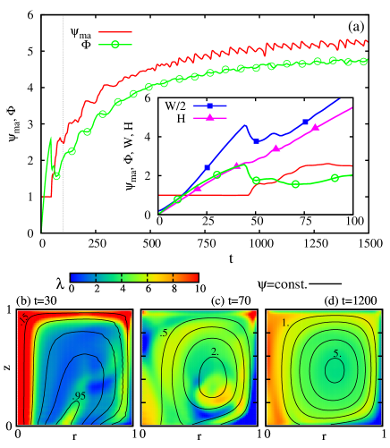
Figure 1: (Color online) Evolution of $\psi_{ma}$ and $\Phi$ (a). In the inset, the evolution for $t<100$ is showed in more detail. In addition the (halved) magnetic energy and the helicity are shown. Colormaps of $\lambda$ and $\psi$ contours in the poloidal plane are shown at three different times (b)-(d).

Panels (b), (c) and (d) of Fig. 1 show contours of $\psi$ and colormaps of $\lambda$ (where $\lambda={\bf J\cdot B}/B^{2}$, is computed using the $n=0$ component of the toroidal Fourier decomposition of ${\bf B}$) at different times. At $t=30$, $\lambda$ is strongly peaked near the geometric axis and no closed $\psi$ contours are identified. After the relaxation event ($t=70$) $\lambda$ is redistributed and closed $\psi$ contours appear, indicating the formation of a spheromak configuration. The poloidal and toroidal fluxes continue to increase until $t\sim 700$ and afterwards a quasi stationary state is sustained for one resistive time, indicating that a balance between helicity injection and dissipation has been reached. The $\psi$ and $\lambda$ distributions shown in Fig. 1 (d) are representative of this quasi-steady state.

It is well known that spheromak formation and sustainment necessarily involves non-axisymmetric activity. The magnetic field lines (followed from fixed positions at the bottom end) plotted in Fig. 2 clearly show that our computations reproduce this feature.

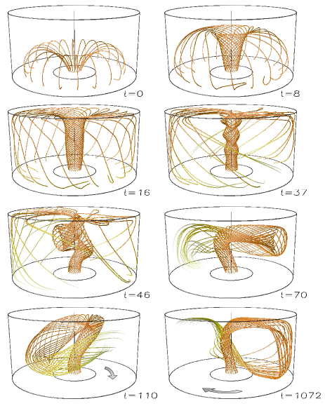
Figure 2: (Color online) Twenty field lines followed from fixed positions at the bottom end, for eight different times. The opacity of the lines is gradually decreased when their length $L$ is longer than $4$, and they become completely transparent when $L\geq 5$. The structure observed at $t=110$ is almost in its final saturated state (observed at $t=1072$) and rotates clockwise (when viewed from top).

The initial field lines of the vacuum solution ($t=0$) expand and twist ($t=8$) forming a central current-carrying column ($t=16$). As the current through the central column increases and the field lines increase their twisting, the configuration eventually becomes unstable ($t=37$) and the typical helical structure of a kink instability quickly develops ($t=46$). This instability, with dominant toroidal wavenumber $n=1$, saturates at a relatively small and fixed amplitude ($W_{n=1}/W_{n=0}\sim 0.01$ during sustainment, see Fig. 4) causing the central column to adopt an almost fixed helical shape which rotates as indicated in Fig. 2 ($t=110$ and $t=1072$). Our results reproduce the experimental observation of a fixed rotating helical structure with a strongly asymmetric return column Duck et al. (1997). In contrast with our case (driven purely by boundary flows), the plasma in those experiments was driven electrostatically. We note, however, that the presence of an inductive component in the electric field when magnetic fluctuations were active, was also reported Duck et al. (1997).

It is important to note that the motion of this structure is produced by the coherent oscillation of the $n=1$ mode and not by a rigid rotation of the plasma. This is shown in Fig. 3 where the radial profiles of $B_{\theta}$ and $B_{z}$, at $z=h/2$ and $\theta=0$, are plotted for several times between $t_{1}=1290$ and $t_{3}=1380$.

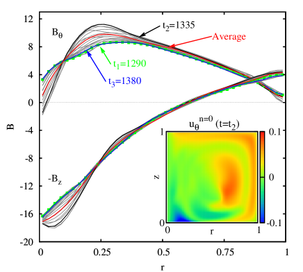
Figure 3: (Color online) Twenty instantaneous profiles (between $t_{1}$ and $t_{3}$) of $B_{\theta}$ and $B_{z}$, at $z=h/2$ and $\theta=0$. The profile of the time averaged fields is also shown. The $n=0$ component of the toroidal velocity at $t_{2}$ is shown in the inset.

The profiles at $t_{1}$ and $t_{3}$ are almost identical, indicating that the structure makes one turn every $90$ Alfvèn times. Such rotation is much slower than that expected from the imposed $u_{0}=-0.1$ at $r=0.2$. Furthermore, the plasma toroidal velocity reverses its sign as can be observed in the inset of Fig. 3 (this velocity colomap is plotted at $t_{2}=1335$ but it is representative of the flow pattern during sustainment, $700<t<1500$). This velocity reversal is also observed in the other two runs presented in this work and it is evidently a feature of the saturated state of the instability. However, the specific reason for this velocity reversal is still not yet understood.

The evolution of $\psi_{ma}$ and the poloidal magnetic field near the wall (total $B_{z}|_{w}$ and $B_{z}^{n=0}|_{w}$) at $z=h/2$ and $\theta=0$ are shown for three values of $u_{0}$ in Fig. 4 (a)-(c). The magnetic energy (relative to the initial energy) of the modes $n=0$, $n=1$ and $n=2$ is shown in Fig. 4 (d). These results indicate that increasing the helicity injection rate (which is linear in $u_{0}$) leads to configurations with higher flux amplification and more energy in the $n=0$ mode.

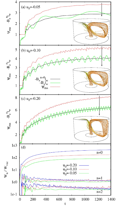
Figure 4: (Color online) Evolution of $\psi_{ma}$ and the poloidal magnetic field near the wall (total $B_{z}|_{w}$ and $B_{z}^{n=0}|_{w}$) for three values of $u_{0}$ (a)-(c). Field lines showing the central open flux column are presented in each case at the time indicated by the arrow. Magnetic energy of the modes $n=0,1$ and $2$ (d).

Nevertheless, the energy associated to the $n>0$ modes (in particular the $n=1$) saturates at a fixed amplitude, which is roughly independent of $u_{0}$. This implies a lower level of fluctuations relative to the $n=0$ mode at higher helicity injection rates. A similar saturation mechanism has also been observed in experiments Duck et al. (1997); Willett et al. (1999).

The oscillation of the fluctuation in the poloidal magnetic field near the wall ($B_{z}|_{w}$) is clearly observed in Figs. 4 (a)-(c). As discussed previously, this corresponds to a coherent oscillation which produces the rotation of the magnetic structures shown in the insets of Figs. 4 (a)-(c). Note that the rotation frequency increases rapidly with the helicity injection rate. Another important observation is that the rotation frequency is not the same, in general, that the frequency of the oscillating dynamo term that amplifies $\psi_{ma}$ (which depends on the correlation of the fluctuations of ${\bf u}$ and ${\bf B}$). This is specially clear in Fig. 4 (b).

The MHD activity maintains the configurations obtained for the three different values of $u_{0}$ close to the kink stability boundary. This is shown in Fig. 5. The $\lambda(\psi)$ profiles of the $n=0$ mode are plotted in Fig. 5 (a), for the case with $u_{0}=-0.1$, at ten times between $t_{1}$ and $t_{3}$ ($\psi$ is normalized with $\psi_{ma}$).

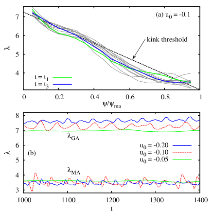
Figure 5: (Color online) $\lambda(\psi)$ profiles for the case with $u_{0}=-0.1$ at ten times between $t_{1}$ and $t_{3}$ (a). The kink instability threshold is indicated. Time evolution of $\lambda$ at the geometric axis ($\lambda_{GA}$) and at the magnetic axis ($\lambda_{MA}$), for the three runs (b).

The indicated kink instability threshold is a linear $\lambda(\psi)$ profile, which has a slope $\alpha=-0.4$ Knox et al. (1986). Fig. 5 (b) shows the evolution of the $\lambda$ values at the geometric axis ($\lambda_{GA}$) and at the magnetic axis ($\lambda_{MA}$) for the three runs. The behavior observed here is similar to that described in previous experiments Knox et al. (1986); Willett et al. (1999). The configuration evolves around the kink stability boundary as a result of the competition between the external forcing, which tends to steepen the $\lambda$ profile, and the relaxation, which tends to flatten it.

In summary, we demonstrated the possibility of forming and sustaining a spheromak by imposing tangential flows at the boundary. Several aspects of the process were described. The relationship between our results and the existing experimental evidence was discussed. The fact that our simulations reproduce many features observed in electrostatic CHI experiments is interpreted as follows. Since the spheromak is formed and sustained by the relaxation of an unstable configuration, the dynamics of the process should be independent of the details on how this configuration is driven unstable. In this sense, this Letter not only provides evidence on a new spheromak formation and sustainment mechanism, but it also provides valuable information pertaining to the dynamics of the kink instability in electrostatically driven spheromaks. To conclude, we note that althought our results were obtained for a spheromak, boundary plasma flows could also be used to inject helicity in other configurations (i.e. spherical tokamaks).