Adaptive information filtering for dynamic recommender systems

Abstract

The dynamic environment in the real world calls for the adaptive techniques for information filtering, namely to provide real-time responses to the changes of system data. Where many incremental algorithms are designed for this purpose, they are usually challenged by the worse and worse performance resulted from the cumulative errors over time. In this Letter, we propose two incremental diffusion-based algorithms for the personalized recommendations, which integrate some pieces of local and fast updatings to achieve the approximate results. In addition to the fast responses, the errors of the proposed algorithms do not cumulate over time, that is to say, the global recomputing is unnecessary. This remarkable advantage is demonstrated by several metrics on algorithmic accuracy for two movie recommender systems and a social bookmarking system.

1 Introduction

The information overloading problem in the Internet era causes many automatic filtering techniques to appear [1], among which the personalized recommender system is a promising one [2, 3, 4]. In the literature, the central problem concerned in the design of recommender systems is how to improve the accuracy [5, 6, 7] and diversity [8, 9, 10] of recommendations. Recently, the well-developed Web 2.0 technique facilitates users to frequently communicate with the system in an easy way, leading to a real-time data flow. How to properly design an incremental algorithm that can adaptively give responses to the changes of data has thus become an urgent problem nowadays. Where some previous studies have already considered such an issue [11, 12, 13, 14, 15, 16, 17], they are challenged by the worse and worse performance resulted from the cumulative errors over time.

Recently, Zhang et al. [18, 19] have successfully applied the classical physical processes, such as the heat conduction and mass diffusion, to deal with the personalized recommendation problem. The original algorithms require a kind of steady states, and to arrive at these states is time consuming. Zhou et al. [10, 20] thus proposed the simplified versions where only one step of heat conduction and/or mass diffusion is taken into account. These simplified algorithms are considerably more accurate than the standard collaborative filtering [21] and much faster yet with competitive accuracy compared with the matrix decomposition techniques [22]. In this Letter, we propose two adaptive algorithms based on the one-step diffusion methods, which integrate some pieces of local updatings and can provide very fast response to each unit change. More significantly, the error between the results of the adaptive algorithms and the static algorithms does not grow larger over time, namely the adaptive algorithms could keep up with the changes tightly and thus no global recomputing is needed. This remarkable feature highlights a new methodology to handle the huge-size dynamic systems, and can avoid the serious problems in the maintaining-retraining scheme [14], like the data synchronization.

2 Static algorithms

A recommender system can be represented by a bipartite network [23], which consists of a user set $\vect{U}$ and an item set $\vect{I}$. To make the description clear, we use lower case letters $i$, $j$, $k$, $\dots$ to index the users and Greek letters $\alpha$, $\beta$, $\gamma$, $\dots$ to index the items. Each user is connected to the items she/he collected, reviewed, voted with high ratings, purchased, etc. Later, we simply use collect/collected to stand for all possible relations between users and items. The bipartite network can be described by an adjacency matrix $\vect{A}=\left\{a_{i\alpha}\right\}$, where $a_{i\alpha}=1$ if an edge between user $i$ and item $\alpha$ exists, $a_{i\alpha}=0$ otherwise.

A diffusion-based recommendation algorithm applies some physical processes to simulate the resource propagation in the bipartite network. For an arbitrary target user, assigning some resources to her/his collected items, whether she/he user will collect certain items in the future can be predicted according to the resource distribution after the diffusion process [20]. Generally speaking, this kind of methods can be formulated as $\vect{f^{\prime}}=\vect{W}\vect{f}$, where $\vect{f}$ is the vector representing the initial resource allocation, $\vect{f^{\prime}}$ is the final resource distribution and $\vect{W}$ is the propagation matrix. Provided the target user $i$, a straightforward way, also adopted in this Letter, is to set the initial vector as $f_{\alpha}=a_{i\alpha}$, namely to assign all the objects collected by user $i$ a unit of resource. The element $w_{\alpha\beta}$ denotes the fraction of item $\beta$’s initial resource that eventually arrives at item $\alpha$. Sorting all uncollected items by $\vect{f^{\prime}}$ in descending order, the ones at the top positions are recommended.

We here consider two simplest diffusion-based algorithms: the one-step mass diffusion (MD) [20] and heat conduction (HC) [10]. The propagation matrix of MD is denoted by $\vect{M}$ with

$$m_{\alpha\beta}=\frac{1}{k_{\beta}}\sum_{i\in\vect{U}}\frac{a_{i\alpha}a_{i\beta}}{k_{i}},$$ (1)

where $k_{i}$ and $k_{\beta}$ are the degrees of user $i$ and item $\beta$, respectively. Analogously, the propagation matrix $\vect{H}$ of HC reads

$$h_{\alpha\beta}=\frac{1}{k_{\alpha}}\sum_{i\in\vect{U}}\frac{a_{i\alpha}a_{i\beta}}{k_{i}}.$$ (2)

Figure 1: (Color online) Illustration of the diffusion processes by MD and HC. (a) and (b) display how a unit of resource initially located on item $\beta$ spreads to item $\alpha$ by MD, while (c) and (d) show how a unit of resource (a physical explanation of this kind of resource is “temperature”, see Refs. [10, 18] for details) initially located on item $\alpha$ spreads to item $\beta$ according to HC. As shown in this figure, $m_{\alpha\beta}=h_{\beta\alpha}=1/4$.

Figure 1 illustrates the processes of MD and HC. Interestingly, the MD and HC are a pair of reverse processes, say $\vect{M}^{T}=\vect{H}$. A direct benefit of this feature is that one only needs to compute one propagation matrix and then immediately gets the other one by transposition, which can reduce the computation when considering the hybrid algorithm involving both the two processes [10]. In this Letter, we will exploit this feature in a more artful way to develop an effective and efficient adaptive algorithm.

3 Exact solution on incremental data

Although the ability to provide accuracy and diverse recommendations of the MD and HC, especially the hybrid version combined these two, has been demonstrated by extensively experimental analysis [10], they are not able to work directly in a dynamic environment where the bipartite network (represented by $\vect{A}$) itself varies moment to moment. A unit change here is defined as the addition of a new edge, whatever it is attached to a new user, a new item, or old ones. Accordingly, the total number of edges, $l$, is naturally a good indication of the state of the evolving system, which is added to all relevant symbols as the superscript if necessary. For example, $k_{\alpha}^{\left(l\right)}$ means the degree of the item $\alpha$ when there are $l$ edges in the network. A cautious yet infeasible method is to recompute every time when a new edge is added to the system. Instead, the purpose of an adaptive algorithm (or say an incremental algorithm) is to derive the recommendation vector $\vect{f^{\prime}}^{(l+1)}$ in a local and fast way that can avoid the global recomputing.

Before the introduction of the approximately adaptive algorithm, we first figure out the exact solution of $\vect{f^{\prime}}^{(l+1)}$ for an arbitrary target user. As stated above, the propagation matrices of MD and HC can be easily derived by each other, so we only present the case for MD, while the one for HC can be analogously obtained without any difficulties. Since for any target user, $\vect{f^{\prime}}^{(l+1)}=\vect{M}^{(l+1)}\vect{f}^{(l+1)}$, and the change of $\vect{f}$ is straightforward, we only focus on the change of $\vect{M}$.

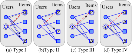
Figure 2: (Color online) Illustration of four types of changes to the $\vect{M}$ with the addition of a new edge. The dotted line is the new edge added between user $i$ and item $\alpha$. The lines with arrow are the diffusion paths affected by the new edge. And the dotted circles emphasize the nodes (users or items) being responsible for the corresponding type of changes.

With the addition of a new edge between user $i$ and item $\alpha$ (we first consider the case that both $i$ and $\alpha$ already exist in the system), the propagation matrix $\vect{M}^{(l)}$ changes to be $\vect{M}^{(l+1)}$. In the microscopic level, the elements of $\vect{M}^{(l+1)}$ can be classified into four types according to the way how they change. As illustrated in Fig. 2, the four types are: Type I—$m_{\beta\alpha}^{\left(l+1\right)}$ where item $\beta$ is connected to user $i$ ($\beta\neq\alpha$). Type II—$m_{\gamma\alpha}^{\left(l+1\right)}$ where item $\alpha$ and $\gamma$ are commonly collected by one or more users rather than the user $i$. Type III—$m_{\alpha\beta}^{\left(l+1\right)}$ where item $\beta$ is connected to user $i$ ($\beta\neq\alpha$). Type IV—$m_{\mu\beta}^{\left(l+1\right)}$ where the item $\beta$ and $\mu$ are both connected to the user $i$ ($\beta\neq\alpha$, $\mu\neq\alpha$).

Denoting by $\delta_{\beta\alpha}^{\left(l+1\right)}$ the change of the element $m_{\beta\alpha}$, say $\delta_{\beta\alpha}^{\left(l+1\right)}=m_{\beta\alpha}^{\left(l+1\right)}-m_{\beta\alpha}^{\left(l\right)}$, according to Fig. 2, it is easy to derive the following updating rules:

$$\delta_{\beta\alpha}^{\left(l+1\right)}=\frac{-1}{k_{\alpha}^{\left(l+1\right)}}m_{\beta\alpha}^{\left(l\right)}+\frac{1}{k_{\alpha}^{\left(l+1\right)}k_{i}^{\left(l+1\right)}}.$$ (3)

$$\delta_{\gamma\alpha}^{\left(l+1\right)}=\frac{-1}{k_{\alpha}^{\left(l+1\right)}}m_{\gamma\alpha}^{\left(l\right)}.$$ (4)

$$\delta_{\alpha\beta}^{\left(l+1\right)}=\frac{1}{k_{\beta}^{\left(l+1\right)}k_{i}^{\left(l+1\right)}}.$$ (5)

$$\delta_{\mu\beta}^{\left(l+1\right)}=\frac{-1}{k_{\beta}^{\left(l+1\right)}k_{i}^{\left(l\right)}k_{i}^{\left(l+1\right)}}.$$ (6)

Table 1: Fundamental statistics of the applied data sets. The data sets for Netflix and Delicious are random samples.

Data Set	$|U|$	$|I|$	Average Object Degree
MovieLens	943	1574	52.43
Netflix	609	8824	11.33
Delicious	1623	32941	3.77

Note that, the updating rules shown in Eqs. (3)-(6) do not change when the addition of the edge introduces a new user of a new item, and only a few extra manipulations are required. When introducing a new user $i$, only type II happens. When a new item $\alpha$ is introduced, a new row and a new column need to be appended to $\vect{M}^{\left(l\right)}$ and initialized to zero, which actually are the initial values of $m_{\beta\alpha}^{\left(l+1\right)}$ and $m_{\alpha\beta}^{\left(l+1\right)}$. In this case the type II won’t happen but type I, type III and type IV should be considered to update the expanded propagation matrix. Finally, when both a new user and a new item are added, no change will be made to the existed elements in $\vect{M}^{\left(l\right)}$. The only operation is to append a new row and a column to $\vect{M}^{\left(l\right)}$ and to initialize them to zero.

We have already numerically checked that the updating rules in Eqs. (3)-(6) can exactly reproduce the results of static algorithm. It seems that there is no need to design another approximated algorithm since all the the changed elements can be handled by Eqs. (3)-(6). Unfortunately, this exact incremental algorithm is facing a dilemma between space and time, and thus far away from the real-world application. In spite of that, the Eqs. (3)-(6) provide a valuable information for analyzing the errors of the adaptive algorithms that will be discussed in the next section.

4 Adaptive algorithms

The compressed storage (only the nonzero elements are stored) of the adjacency matrix makes it difficult to be randomly accessed, however, calculating the propagation from a certain item to the others, whether by mass diffusion or heat conduction, is very efficient in such infrastructure, because it can access the adjacency matrix (or equivalent data structure representing the connections between users and items) in a sequential way. Hence, for the elements belonging to Type I and Type II, instead of identifying and updating, one can just redo a mass diffusion starting with the item $\alpha$ to get the updated values. We call this algorithm the adaptive algorithm with first-order approximation, abbreviated as AAF.

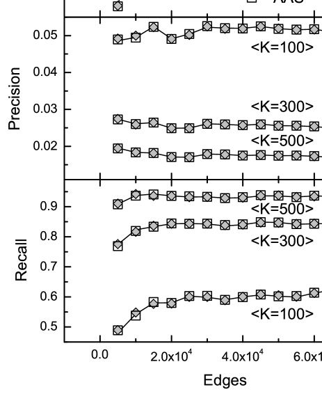
Figure 3: AUC, Precision and Recall as the function of the number of edges fed to the algorithms on MovieLens data. The algorithm starts with 5000 edges. Precision and Recall are evaluated with $K=100$, $300$ and $500$, respectively. For all numerical results, including the ones shown in Fig. 4 and Fig. 5, the solid lines represent the results of static algorithm, and the diamonds and squares correspond to AAF and AAS.

In AAF, when an edge is added, only the elements belonging to the first and the second types are updated by using the MD starting from the item $\alpha$. The high efficiency is guaranteed, whereas the error is introduced for the neglect of other changes of Type III and Type IV. Detailedly, an error of $\left(k_{\beta}^{\left(l+1\right)}k_{i}^{\left(l+1\right)}\right)^{-1}$ (see Eq. (5)) occurs when an element in the third type is not updated, and an error of $\left(k_{\beta}^{\left(l+1\right)}k_{i}^{\left(l\right)}k_{i}^{\left(l+1\right)}\right)^{-1}$ (see Eq. (6)) occurs when an element in the fourth type is not updated. Obviously, the latter error is far less than the former one since in a real system, many users have collected more than a hundred items. Therefore, if the error of the elements in the third type can be eliminated, the accuracy of the approximate algorithm will be improved significantly.

The straightforward way to update the elements in the third type will add too much computation burden, because it needs to simulate the MD process from all items sharing at least one common neighboring user with the item $\alpha$ to the item $\alpha$ (see Eq. (5)). Thanks to the reversibility found for the MD and HC processes, we conquer this difficulty skillfully. Instead of MD, an HC process starting from the item $\alpha$ is calculated in $\vect{A}^{\left(l+1\right)}$, then the resource arriving at item $\beta$ is $m_{\alpha\beta}^{\left(l+1\right)}$. By this way, the updating of all the elements in the third type is completed by HC once from one item, with the same complexity as in AAF. We name this algorithm as the adaptive algorithm with second-order approximation, abbreviated as AAS. In AAS, when an edge to the item $\alpha$ is added, an MD from the item $\alpha$ is done to get the updated elements in the first and the second types, then an HC from the item $\alpha$ is done to get the updated elements in the third type.

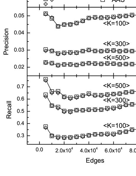
Figure 4: AUC, Precision and Recall as the function of the number of edges fed to the algorithms on Netflix data. The algorithm starts with 5000 edges. Precision and Recall are evaluated with $K=100$, $300$ and $500$, respectively.

5 Experimental results

To validate that the proposed adaptive algorithms could provide good approximation for the static algorithm, we run numerical simulations on three real systems: MovieLens, Netflix, and Delicious. The characteristics of these data sets are summarized in Table 1. The original data of MovieLens and Netflix record the opinions of users on items with the ratings from 1 (the worst) to 5 (the best). We convert these two rating systems to binary systems by defining a connection between a user and an item only if the corresponding rating is higher than 2.

A standard sub-sampling validation method is adopted to evaluate the algorithmic performance, which divides all edges randomly into two subsets: the training set and the testing set. The training set is used as the known information for recommending, while the testing set is used to evaluate the prediction and is invisible to the recommendation algorithms. In this Letter, $10\%$ of edges constitute the testing set and the other $90\%$ belong to the training set. Three widely measurements, AUC, Precision and Recall, are applied to quantify the accuracy of recommendations (see the review article [5] for details). All of them are essentially individual-based indices, that is to say, for any user $i$, the individual measurements $AUC_{i}^{\left(l\right)}$, $Precision_{i}^{\left(l\right)}$ and $Recall_{i}^{\left(l\right)}$ exist. The system-level indices are simply obtained by averaging the individual measurements over all users. Denoting by $T_{i}^{(l)}$ the set of items in the testing set that are collected by user $i$ (they are invisible from the training set but favored by user $i$), and $F_{i}^{(l)}=\vect{I}^{(l)}-\Gamma_{i}^{(l)}-T_{i}^{(l)}$ the set of items not favored yet by user $i$, where $\Gamma_{i}^{(l)}$ is the set of items collected by user $i$ in the training set, then $AUC_{i}^{(l)}$ is defined as the probability a randomly selected item in $T_{i}^{(l)}$ is assigned a topper position in the recommendation list than a randomly selected item in $F_{i}^{(l)}$. Clearly, random recommendations correspond to $AUC\approx 0.5$. Given the length of recommendation list, $K$, the $Precision_{i}^{\left(l\right)}$ is defined as the ratio of the number of the recommended items belonging to $T_{i}^{\left(l\right)}$ to the total of recommended items, $K$. The $Recall_{i}^{\left(l\right)}$ is the ratio of the number of the recommended items belonging to $T_{i}^{\left(l\right)}$ to $|T_{i}^{\left(l\right)}|$. Note that, AUC value does not depend on $K$, while the Precision and Recall are $K$-sensitive. For all these three indices, the larger value corresponds to the higher recommendation accuracy.

To imitate the dynamic environment in the real world, we sort the edges in the training set by the time when they appeared, then feed them to the algorithm one by one. For each 5000 edges, we compute the AUC, Precision and Recall. The performance along with the adding of edges is shown in Figs. 3-5. As the addition of edges, the known information increases and thus the AUC value increases too. In contrast, the Precision and Recall exhibit larger irregularities since they concentrate on a tiny fraction of items (i.e., top-recommended items). For both the three indices, the adaptive algorithms perform well, even when the Precision and Recall of the static algorithm displaying irregularities, the approximated algorithms accurately reproduce these irregularities. In addition, it is seen that the AAS performs better than the AAF especially for the sparser data sets, Netflix and Delicious.

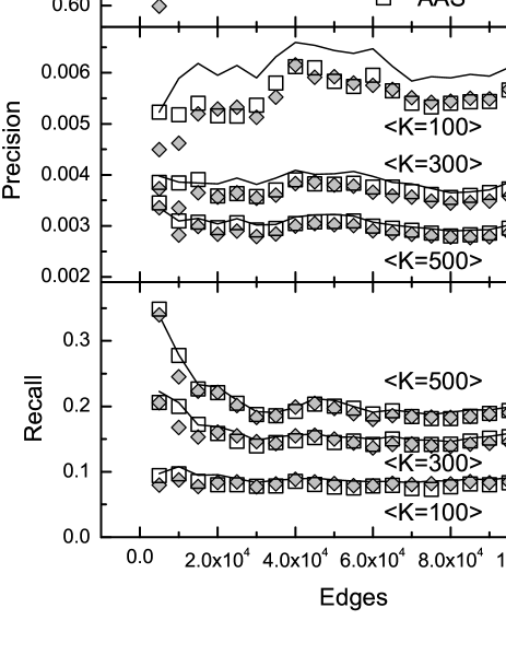
Figure 5: AUC, Precision and Recall as the function of the number of edges fed to the algorithms on Delicious data. The algorithm starts with 5000 edges. Precision and Recall are evaluated with $K=100$, $300$ and $500$, respectively.

The most significant feature of the adaptive algorithms, AAF and AAS, is that they could follow the static algorithm tightly. For MovieLens and Netflix data, almost no difference between the adaptive algorithms and the static algorithm is observed, except a small departure of the AUC for the Netflix data in the start. Even for the Delicious data where there are observable errors of the approximations, the difference does not grow larger over time. This feature strongly encourages the usage of AAS to completely replace the costly static algorithm. It is worthwhile to emphasize that the adaptive algorithms will give more closer results to the static algorithm for denser data, since the error magnitude is negatively correlated with the item degree and user degree (for AAF, see Eq. (5) and Eq. (6); for AAS, see Eq. (6)). One may doubt that although the error caused by the fourth type is small, its accumulative effects may be considerable and make the approximation farther and farther to the static algorithm. Fortunately, this will never happen in real systems because when a new edge adjacent to an item $\alpha$ is added, all the errors of the elements of $\vect{M}$ relevant to $\alpha$ (i.e., $m_{\alpha\cdot}$ and $m_{\cdot\alpha}$) will be eliminated by AAS. Therefore, the errors relevant to active items will not cumulate, while the items rarely attaching new connections must be less attractive or out of date, which contribute very little to the recommendations.

6 Conclusion and Discussion

Although new data comes every moment, many information filtering systems still adopt the traditionally algorithmic framework, which periodically recompute on the whole data. Under the dynamic environment of data flow, an urgent problem is how to design effective and efficient adaptive algorithms to give real-time responses to the change of data. A well-designed algorithm is supposed to not only provide fast and accurate responses, but also avoid the cumulative increase of errors, so that the global recomputation is unnecessary. However, for a general static recommendation algorithm, there is no guarantee of the existence of such an adaptive algorithm. In this Letter, being aware of the reversibility of mass diffusion and heat conduction, we propose a fast and accurate adaptive algorithm with second-order approximation, which could follow the static algorithm very tightly and avoid the cumulative growth of errors.

Although this Letter only presented the adaptive algorithms for mass diffusion process, the heat conduction process can be handled in an analogous way. Moreover, the linear integration of mass diffusion and heat conduction is shown to be able to provide much more accurate and diverse recommendations than either single algorithm [10]. The proposed AAS can be straightforwardly extended to deal with this linear hybrid case. The present method can also find its applications for more complicated diffusion-based recommendation algorithms, for example, the diffusions on multi-rating systems [19, 24] or hypergraphs involving users, items and tags [25, 26].

- [1] \NameHanani U., Shapira B. Shoval P. \REVIEWUser Mod. User-Adap. Interact.112001203.
- [2] \NamePazzani M. J. \REVIEWArtif. Intell. Rev.131999393.
- [3] \NameGoldberg D., Nichols D., Oki B. M., Terry D. \REVIEWCommun. ACM35199261.
- [4] \NameResnick P. Varian H. R. \REVIEWCommun. ACM40199756.
- [5] \NameHerlocker J. L., Konstan J. A., Terveen L. G. Riedl J. T. \REVIEWACM Trans. Inf. Syst.2220045.
- [6] \NameAdomavicius G. Tuzhilin A. \REVIEWIEEE Trans. Knowl. Data Eng.172005734.
- [7] \NameBennett J. Lanning S. Proc. KDD Cup Workshop (ACM Press, New York) 2007, pp. 3-6.
- [8] \NameZhou T., Jiang L.-L., Su R.-Q. Zhang Y.-C. \REVIEWEurophys. Lett.81200858004.
- [9] \NameZhou T., Su R.-Q., Liu R.-R., Jiang L.-L., Wang B.-H. Zhang Y.-C. \REVIEWNew J. Phys.to be published
- [10] \NameZhou T., Kuscsik Z., Liu J.-G., Medo M., Wakeling J. R. Zhang Y.-C. arXiv: 0808.2672.
- [11] \NameMiranda C. Jorge A. M. Proc. the 1st Workshop on Web and Text Intell. (ICMC/USP, Sao Carlos) 2008, pp. 35-42.
- [12] \NameCoster R. Svensson M. Proc. the 2005 ACM Sym. on Appl. Comp. (ACM Press, New York) 2005, pp. 1102-1106.
- [13] \NameGeogre T. Merugu S. Proc. the 5th IEEE Int. Conf. on Data Mining (IEEE Computer Society Press, Washington DC) 2005, pp. 625-628.
- [14] \NameSuryavanshi B. S., Shiri N. Mudur S. P. Proc. WebKDD Workshop on Tam. Evo., Expan. and Mul.-face. Web Cli. (ACM Press, New York) 2005, pp. 44-55.
- [15] \NameSarwar B., Karypis G., Konstan J. Riedl J. 5th Int. Conf. on Com. and Info. Tech. (IEEE Computer Society Press, Washington DC) 2002, pp. 27-28.
- [16] \NameWu H., Wang Y.-J. Cheng X. Proc. of the ACM Conf. on Recomm. Syst. (ACM Press, New York) 2008, pp. 99-106.
- [17] \NameAlSumait L., Barbara D. Domeniconi C. Proc. of 8th IEEE Int. Conf. on Data Min. (IEEE Computer Society Press, Washington DC) 2008, pp. 3-12.
- [18] \NameZhang Y.-C., Blattner M. Yu Y.-K. \REVIEWPhys. Rev. Lett.992007154301.
- [19] \NameZhang Y.-C., Medo M., Ren J., Zhou T., Li T. Yang F. \REVIEWEurophys. Lett.80200768003.
- [20] \NameZhou T., Ren J., Medo M. Zhang Y.-C. \REVIEWPhys. Rev. E762007046115.
- [21] \NameBreese J. S., Heckerman D. Kadie C. Proc. 14th Int. Conf. Uncertainty in Artif. Intell. (Morgan Kaufmann, Madison) 1998, pp. 43-52.
- [22] \NameRen J., Zhou T. Zhang Y.-C. \REVIEWEurophys. Lett.82200858007
- [23] \NameShang M.-S., Lü L., Zhang Y.-C. Zhou T. arXiv: 0909.4938.
- [24] \NameShang M.-S., Jin C.-H., Zhou T. Zhang Y.-C. \REVIEWPhysica A38820094867.
- [25] \NameZhang Z.-K., Zhou T. Zhang Y.-C. \REVIEWPhysica A3892010179.
- [26] \NameShang M.-S. Zhang Z.-K. \REVIEWChin. Phys. Lett.262009118903