Quantum transport of strongly interacting photons in a one-dimensional nonlinear waveguide

Abstract

We present a theoretical technique for solving the quantum transport problem of a few photons through a one-dimensional, strongly nonlinear waveguide. We specifically consider the situation where the evolution of the optical field is governed by the quantum nonlinear Schrödinger equation (NLSE). Although this kind of nonlinearity is quite general, we focus on a realistic implementation involving cold atoms loaded in a hollow-core optical fiber, where the atomic system provides a tunable nonlinearity that can be large even at a single-photon level. In particular, we show that when the interaction between photons is effectively repulsive, the transmission of multi-photon components of the field is suppressed. This leads to anti-bunching of the transmitted light and indicates that the system acts as a single-photon switch. On the other hand, in the case of attractive interaction, the system can exhibit either anti-bunching or bunching, which is in stark contrast to semiclassical calculations. We show that the bunching behavior is related to the resonant excitation of bound states of photons inside the system.

I Introduction

Physical systems that enable single photons to interact strongly with each other are extremely valuable for many emerging applications. Such systems are expected to facilitate the construction of single-photon switches and transistors Birnbaum et al. (2005); Schuster et al. (2008); Chang et al. (2007), networks for quantum information processing, the realization of strongly correlated quantum systems using light Hartmann et al. (2006); Greentree et al. (2006); Chang et al. (2008) and the investigation of novel new many-body physics such as out of equilibrium behaviors. One potential approach involves the use of high-finesse optical microcavities containing a small number of resonant atoms that mediate the interaction between photons Raimond et al. (2001); Birnbaum et al. (2005). Their nonlinear properties are relatively straightforward to analyze or simulate because they involve very few degrees of freedom (i.e., a single optical mode) Imamoglu et al. (1997); Grangier et al. (1998); Imamoglu et al. (1998). Recently, an alternative approach has been suggested, involving the use of an ensemble of atoms coupled to propagating photons in one-dimensional, tightly-confining optical waveguides Ghosh et al. (2005); Kien and Hakuta (2008); Akimov et al. (2008). Here, the nonlinearities are enhanced due to the transverse confinement of photons near the diffraction limit and the subsequent increase in the atom-photon interaction strength. The propagation of an optical field inside such a nonlinear medium (e.g., systems obeying the quantum nonlinear Schrödinger equation) is expected to yield much richer effects than the case of an optical cavity due to the large number of spatial degrees of freedom available. Simultaneously, however, these degrees of freedom make analysis much more difficult and in part cause these systems to remain relatively unexplored Lai and Haus (1989a); Kärtner and Haus (1993); Drummond (2001); Shen and Fan (2007); Chang et al. (2008). We show that the multi-mode, quantum nature of the system plays an important role and results in phenomena that have no analogue in either single-mode cavities or classical nonlinear optics. It is interesting to note that similar low-dimensional, strongly interacting condensed matter systems are an active area of research, but most of this work is focused on closed systems close to the ground state or in thermal equilibrium Lieb and Liniger (1963); Korepin et al. (1993); Kinoshita et al. (2004); Parades et al. (2004); Calabrese and Caux (2007). On the other hand, as will be seen here, the relevant regime for photons often involves open systems and driven dynamics.

In this article, we develop a technique to study the quantum transport of a few photons inside a finite-length, strongly nonlinear waveguide where the light propagation is governed by the quantum nonlinear Schrödinger equation (NLSE), and apply this technique to study the operation of this system as a single-photon switch. In particular, we study the transmission and reflection properties of multi-photon fields from the system as well as higher-order correlation functions of these fields. We find that these correlations not only reflect the switching behavior, but reveal some aspects of the rich structure associated with the spatial degrees of freedom inside the system, which allow photons to “organize” themselves. In the regime where an effectively repulsive interaction between photons is achieved, anti-bunching in the transmitted field is observed because of the switching effect, and is further reinforced by the tendency of photons to repel each other. In the attractive regime, either anti-bunching (due to switching) or bunching can occur. We show that the latter phenomenon is a clear signature of the creation of photonic bound states in the medium. Although we focus on a particular realization involving the propagation of light, our conclusions on quantum transport properties are quite general and valid for any bosonic system obeying the NLSE.

This article is organized as follows. In Sec. II, we describe an atomic system whose interactions with an optical field can be manipulated using quantum optical techniques such that the light propagation obeys the quantum NLSE. This method relies upon electromagnetically induced transparency (EIT) to achieve resonantly enhanced optical nonlinearities with low propagation losses and the trapping of stationary light pulses using spatially modulated control fields. Before treating the nonlinear properties of the system, we first consider the linear case in Sec. III, where it is shown that the light trapping technique leads to a field build-up inside the medium and a set of discrete transmission resonances, much like an optical cavity. In Sec. IV, we then investigate the nonlinear transport properties of the system such as reflectivity and transmittivity in the semi-classical limit, where the NLSE is treated as a simple complex differential equation. Here we find that the presence of the nonlinearity causes the transmission resonances to shift in an intensity-dependent way – the system behaves as a low-power, nonlinear optical switch, whose behavior does not depend on the sign of the nonlinear interaction. In Sec. V, we present a full quantum formalism to treat the NLSE transport problem in the few-photon limit. Sec. VI is dedicated to analytical solutions of the NLSE with open boundary conditions when the system is not driven. In particular, we generalize the Bethe ansatz technique to find the resonant modes of the system, which help to elucidate the dynamics in the case of the driven system. The driven system is studied in Sec. VII, where numerical solutions are presented along with a detailed study of the different regimes of behavior. In particular, we find that the correlation functions for the transmitted light do depend on the sign of the nonlinear interaction, in contrast to what the semi-classical calculations would suggest. We conclude in Sec. VIII.

II Model: Photonic NLSE in 1D waveguide

In this section, we consider the propagation of light inside an finite-length atomic medium under EIT conditions and with a Kerr nonlinearity. We also describe a technique that allows for these pulses of light to be trapped within the medium using an effective Bragg grating formed by additional counter-propagating optical control fields. We show that in the limit of large optical depth the evolution of the system can be described by a nonlinear Schrödinger equation.

Following Ref. Chang et al. (2008), we consider an ensemble of atoms with the four-level internal structure shown in Fig. 1, which interact with counter-propagating quantum fields with slowly-varying envelopes $\hat{\mathcal{E}}_{\pm}$ inside an optical waveguide. These fields are coupled to a spin coherence between states $|a\rangle$ and $|c\rangle$ via two classical, counter-propagating control fields with Rabi frequencies $\Omega_{\pm}$ largely detuned from the $|b\rangle\rightarrow|c\rangle$ transition. The case where the fields propagate only in one direction (say in the “+” direction) and where the detuning is zero corresponds to the usual EIT system, where the atomic medium becomes transparent to $\hat{\mathcal{E}}_{+}$ and the group velocity can be dramatically slowed due to coupling between the light and spin wave (so-called “dark-state polaritons”) Fleischhauer and Lukin (2000). On the other hand, the presence of counter-propagating control fields creates an effective Bragg grating that causes the fields $\hat{\mathcal{E}}_{\pm}$ to scatter into each other. This can modify the photonic density of states and create a bandgap for the quantum fields. This photonic bandgap prevents a pulse of light from propagating and can be used to effectively trap the light inside the waveguide André and Lukin (2002); Bajcsy et al. (2003). The trapping phenomenon is crucial because it increases the time over which photons can interact inside the medium. The presence of an additional, far-detuned transition $|c\rangle\rightarrow|d\rangle$ that is coupled to $\hat{\mathcal{E}}_{\pm}$ leads to an intensity-dependent energy shift of level $|c\rangle$, which translates into a Kerr-type optical nonlinearity Schmidt and Imamoglu (1996).

We now derive the evolution equations for the quantum fields. We assume that all atoms are initially in their ground states $|a\rangle$. To describe the quantum properties of the atomic polarization, we define collective, slowly-varying atomic operators, averaged over small but macroscopic volumes containing $N_{z}\gg 1$ particles at position $z$,

$$\hat{\sigma}_{\alpha\beta}(z,t)=\frac{1}{N_{z}}\sum_{i=1}^{N_{z}}|\alpha_{i}\rangle\langle\beta_{i}|.$$ (1)

The collective atomic operators obey the following commutation relations,

$$[\hat{\sigma}_{\alpha\beta}(z),\hat{\sigma}_{\mu\nu}(z^{\prime})]=\frac{L}{N}\delta(z-z^{\prime})(\delta_{\beta\mu}\hat{\sigma}_{\alpha\nu}(z)-\delta_{\alpha\nu}\hat{\sigma}_{\mu\beta}(z)),$$ (2)

while the forward and backward quantized probe fields in the ${\rm{z}}$ direction obey bosonic commutation relations (at equal time),

$$[\mathcal{\hat{E}}_{+}(z),\mathcal{\hat{E}}_{+}^{\dagger}(z^{\prime})]=\delta(z-z^{\prime}).$$ (3)

The Hamiltonian for this system in the rotating frame can be written as

$$\hat{H}= - \frac{N}{L}\int[\hat{\sigma}_{bc}(z)(\Omega_{+}e^{ik_{c}z}+\Omega_{-}e^{-ik_{c}z})+H.c.]$$

$$+ g\sqrt{2\pi}[\hat{\sigma}_{ba}(z)(\mathcal{\hat{E}}_{+}e^{ik_{0}z}+\mathcal{\hat{E}}_{-}e^{-ik_{0}z})+H.c.]$$

$$+ g\sqrt{2\pi}[\hat{\sigma}_{dc}(z)(\mathcal{\hat{E}}_{+}e^{ik_{0}z}+\mathcal{\hat{E}}_{-}e^{-ik_{0}z})+H.c.]$$

$$+ \Delta_{1}\hat{\sigma}_{bb}(z)+\Delta_{3}\hat{\sigma}_{cc}(z)+(\Delta_{2}+\Delta_{3})\hat{\sigma}_{dd}(z)dz$$

where $g=\mu\sqrt{\frac{\omega_{ab}}{4\pi\hbar\epsilon_{0}A}}$ is the atom-field coupling strength, $\mu$ is the atomic dipole matrix element, and $A$ is the effective area of the waveguide modes. For simplicity, we have assumed that the transitions $a$-$b$ and $c$-$d$ have identical coupling strengths $g$ and have ignored transverse variation in the fields. The terms $\Delta_{i}$ denote the light field-atomic transition detunings as shown in Fig. 1(a). $k_{c}$ is the wavevector of the control fields, while $k_{0}=n_{b}\omega_{ab}/c$ characterizes the fast-varying component of the quantum field and $n_{b}$ is the background refractive index. We also define $n_{0}=N/L$ as the linear density of atoms in the ${\rm{z}}$ direction, and $v_{g}=c\Omega^{2}/2{\pi}g^{2}n_{0}$ as the group velocity that the quantum fields would have if they were not trapped by the Bragg grating (we will specifically be interested in the situation where $\Omega_{+}=\Omega_{-}=\Omega$). Following Ref. Fleischhauer and Lukin (2000), we can define dark-state polariton operators that describe the collective excitation of field and atomic spin wave, which in the limit of slow group velocity $\eta=\frac{c}{2v_{g}}\gg 1$ are given by $\hat{\Psi}_{\pm}=\frac{g\sqrt{2\pi n_{0}}}{\Omega_{\pm}}\mathcal{\hat{E}}_{\pm}$. These operators obey bosonic commutation relations $[\hat{\Psi}_{\pm}(z),\hat{\Psi}_{\pm}^{\dagger}(z^{\prime})]=\delta(z-z^{\prime})$. The definition of the polariton operators specifies that the photon flux entering the system at its boundary is equal to the rate that polaritons are created at the boundary inside the system – i.e., $c\langle\mathcal{\hat{E}_{+}}^{\dagger}\mathcal{\hat{E}_{+}}\rangle=v_{g}\langle\hat{\Psi}_{+}^{\dagger}\hat{\Psi}_{+}\rangle$. In other words, excitations enter (and leave) the system as photons with velocity $c$, but inside the waveguide they are immediately converted into polariton excitations with group velocity $v_{g}$. Field correlations will also be mapped in a similar fashion – in particular, correlation functions that we calculate for polaritons at the end of the waveguide $z=L$ will also hold for the photons transmitted from the system. The total number of polaritons in the system is given by $\mathcal{N}_{pol.}=\int\langle\hat{\Psi}_{+}^{\dagger}\hat{\Psi}_{+}\rangle+\langle\hat{\Psi}_{-}^{\dagger}\hat{\Psi}_{-}\rangle dz$. The optical fields coupled to the atomic coherences of both the $a-b$ and $c-d$ transitions are governed by Maxwell-Bloch evolution equations,

$$\left(\frac{\partial}{\partial t}\pm c\frac{\partial}{\partial z}\right)\mathcal{\hat{E}}_{\pm}(z,t)=ig\sqrt{2\pi}n_{0}(\hat{\sigma}_{ab}+\hat{\sigma}_{cd}).$$ (5)

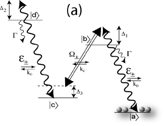
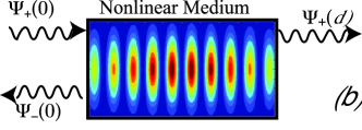
Figure 1: (a) Four-level atomic system for creating strong nonlinearity. Counter-propagating control fields modulate the EIT for the forward- and backward-propagating probe, and $|c\rangle\rightarrow|d\rangle$ transition gives rise to a Kerr-type nonlinearity. (b) The light is confined in the transverse direction due to the presence of the waveguide and experiences an effective Bragg grating due to the presence of the counter-propagating light.

Similar to the photonic operators, the atomic coherences can also be written in terms of slowly-varying components,

$$\hat{\sigma}_{ab} = \hat{\sigma}_{ab}^{+}e^{ik_{0}z}+\hat{\sigma}_{ab}^{-}e^{-ik_{0}z},$$ (6)

$$\hat{\sigma}_{cd} = \hat{\sigma}_{cd}^{+}e^{ik_{0}z}+\hat{\sigma}_{cd}^{-}e^{-ik_{0}z}.$$ (7)

We note that higher spatial orders of the coherence are thus neglected. In practice, these higher orders are destroyed due to atomic motion and collisions as atoms travel distances greater than an optical wavelength during the typical time of the experiment Zimmer et al. (2006). Alternatively, one can use dual-V atomic systems that do not require this approximation Zimmer et al. (2008).

In the weak excitation limit $(\hat{\sigma}_{aa}\simeq 1)$, the population in the excited state $|b\rangle$ can be neglected, $\langle\hat{\sigma}_{bb}\rangle{\approx}0$. In this limit, the evolution of the atomic coherence is given by

$$\dot{\hat{\sigma}}_{ab}^{\pm} = (i\Delta_{1}-\Gamma/2)\hat{\sigma}_{ab}^{\pm}$$

$$+ ig\sqrt{2\pi}\mathcal{\hat{E}}_{\pm}+i\Omega_{\pm}\hat{\sigma}_{ac}e^{\pm i\Delta kz}$$

where $\Delta k=k_{c}-k_{0}$ and $\Gamma$ is the total spontaneous emission rate of state $b$ (for simplicity we also assume that state $d$ has an equal spontaneous emission rate). In the adiabatic limit where $g\sqrt{2\pi}\langle\hat{\sigma}_{ac}\mathcal{\hat{E}}_{\pm}\rangle\ll\Gamma$, the coherence $\hat{\sigma}_{ad}$ can be approximated by

$$\hat{\sigma}_{ad}\simeq\frac{g\sqrt{2\pi}\hat{\sigma}_{ac}}{-\Delta_{2}-\Delta_{3}-i\frac{\Gamma}{2}}(\mathcal{\hat{E}}_{+}e^{+ik_{0}z}+\mathcal{\hat{E}}_{-}e^{-ik_{0}z}).$$ (9)

Therefore, the spin wave evolution can be written as,

$$\dot{\hat{\sigma}}_{ac} = i\Delta_{3}\hat{\sigma}_{ac}+i(\hat{\sigma}_{ab}^{+}\Omega_{+}^{*}e^{-i\Delta kz}+\hat{\sigma}_{ab}^{-}\Omega_{-}^{*}e^{i\Delta kz})$$ (10)

$$+ \frac{2\pi ig^{2}}{-\Delta_{2}-\Delta_{3}-i\frac{\Gamma}{2}}(\mathcal{\hat{E}}_{+}^{\dagger}\mathcal{\hat{E}}_{+}+\mathcal{\hat{E}}_{-}^{\dagger}\mathcal{\hat{E}}_{-})\hat{\sigma}_{ac}$$

We now consider the situation where $\Omega_{+}=\Omega_{-}=\Omega$, such that the counter-propagating control fields form a standing wave. In the adiabatic limit Fleischhauer and Lukin (2000), and keeping all terms up to third order in the quantum fields, substituting these results into Eq. (5) and simplifying yields the following evolution equations for the dark-state polariton operators,

$$(c\partial_{z}+\partial_{t})\hat{\Psi}_{+} = -\frac{\xi}{2}(\hat{\Psi}_{+}-\hat{\Psi}_{-})-\frac{\eta}{2}\partial_{t}(\hat{\Psi}_{+}+\hat{\Psi}_{-})$$ (11)

$$- i\Delta_{n}[(\hat{\Psi}_{+}^{\dagger}\hat{\Psi}_{+}+\hat{\Psi}_{-}^{\dagger}\hat{\Psi}_{-})(\hat{\Psi}_{+}+\hat{\Psi}_{-})$$

$$+ (\hat{\Psi}_{+}^{\dagger}+\hat{\Psi}_{-}^{\dagger})(\hat{\Psi}_{+}+\hat{\Psi}_{-})\hat{\Psi}_{+}]$$

$$(-c\partial_{z}+\partial_{t})\hat{\Psi}_{-} = +\frac{\xi}{2}(\hat{\Psi}_{+}-\hat{\Psi}_{-})-\frac{\eta}{2}\partial_{t}(\hat{\Psi}_{+}+\hat{\Psi}_{-})$$ (12)

$$- i\Delta_{n}[(\hat{\Psi}_{+}^{\dagger}\hat{\Psi}_{+}+\hat{\Psi}_{-}^{\dagger}\hat{\Psi}_{-})(\hat{\Psi}_{+}+\hat{\Psi}_{-})$$

$$+ (\hat{\Psi}_{+}^{\dagger}+\hat{\Psi}_{-}^{\dagger})(\hat{\Psi}_{+}+\hat{\Psi}_{-})\hat{\Psi}_{-}],$$

where the linear dispersion is characterized by $\xi=\frac{2\pi g^{2}n_{0}}{-i\Delta_{1}+\Gamma/2}$ . The nonlinearity coefficient is given by the single photon AC-Stark shift: $\Delta_{n}=\frac{\pi g^{2}}{2(\Delta_{2}+i\Gamma/2)}$. We note that the wave-vector mismatch $\Delta k$ has been compensated for by a small extra two-photon detuning equal to $(-\Delta kc/\eta)$.

The above equations describe the evolution of two coupled modes. It is convenient to re-write these equations in terms of the anti-symmetric and symmetric combinations $A=(\Psi_{+}-\Psi_{-})/\sqrt{2}$ and $S=(\Psi_{+}+\Psi_{-})/\sqrt{2}$. For large optical depths, we then find that the anti-symmetric mode adiabatically follows the symmetric mode, $A\simeq-(c/\xi)\partial_{z}S$. In this limit, the evolution of the whole system can be described by a single nonlinear Schrödinger equation,

$$\eta\frac{\partial}{\partial t}S-\frac{c^{2}}{\xi}\frac{\partial^{2}}{\partial z^{2}}S+8i\Delta_{n}S^{\dagger}S^{2}=0.$$ (13)

Physically, the coupling between $\hat{\Psi}_{\pm}$ induced by the Bragg grating causes them to no longer behave independently, much like the two counter-propagating components of an optical cavity mode. We can write the above equation in dimensionless units by introducing a characteristic length scale $L_{coh}=c/|{\rm{Im}[\xi]|=c(\Delta_{1}^{2}+\Gamma{}^{2}/4)/2\pi g^{2}n_{0}|\Delta_{1}|}$ and time scale $t_{coh}=\eta/|{\rm{Im}[\xi]|=(\Delta_{1}^{2}+\Gamma{}^{2}/4)/2\Omega^{2}|\Delta_{1}|}$. $L_{coh}$ corresponds to the length over which the field acquires a $\pi$-phase in the propagation. The dimensionless NLSE then reads

$$i\frac{\partial\tilde{S}}{\partial\tau}=-\frac{1}{2m}\frac{\partial^{2}\tilde{S}}{\partial\tilde{z}^{2}}+2\kappa\tilde{S}^{\dagger}\tilde{S}^{2},$$ (14)

where for $\Delta_{1}<0$, the effective mass is $m=\frac{1}{2}(1+i\frac{\Gamma}{2|\Delta_{1}|})$ and the nonlinearity coefficient is $\kappa=\frac{2\Delta_{n}}{c}=\frac{\pi g^{2}/c}{\Delta_{2}+i\Gamma/2}$. Note that $\tilde{\Psi}_{\pm}(z,t)$ and $\tilde{S}(z,t)$ are also in units of $\sqrt{L_{coh}^{-1}}$, such that $[\tilde{S}_{+}(\tilde{z}),\tilde{S}_{+}^{\dagger}(\tilde{z}^{\prime})]=\delta(\tilde{z}-\tilde{z}^{\prime})$. For simplicity, we omit tilde superscripts in the following. We can also write the nonlinear coefficient as $\kappa=\frac{\Gamma_{1D}}{4(\Delta_{2}+i\Gamma/2)}$, where we have identified $\Gamma_{1D}=4\pi g^{2}/c$ as the spontaneous emission rate into the guided modes ($\Gamma_{1D}{\leq}\Gamma$). We are primarily interested in the limit $|\Delta_{1,2}|{\gg}\Gamma$ such that $m,\kappa$ are mostly real and the evolution is dispersive. Note that in this notation, the anti-symmetric combination of forward and backward polaritons is given by $A\simeq-i/2m\partial_{z}S\simeq-i\partial_{z}S$.

III Linear case: Stationary light enhancement

In this section, we investigate the linear transmission properties of the signal field as a function of its frequency. The control field leads to a Bragg grating that couples the forward and backward components of the signal field together. We show that the system therefore acts as an effective cavity whose finesse is determined by the optical density of the atomic medium.

For the linear case ($\kappa=0$), it is sufficient to treat the forward and backward field operators as two complex numbers. In the slow light regime ($\eta\gg 1$), the coupled mode equations (Eqs. 12) can be written in the Fourier domain, with our dimensionless units, as

$$\partial_{z}\Phi_{+} = \frac{i}{2}\delta(\Phi_{+}+\Phi_{-})+im(\Phi_{+}-\Phi_{-})$$ (15)

$$-\partial_{z}\Phi_{-} = \frac{i}{2}\delta(\Phi_{+}+\Phi_{-})-im(\Phi_{+}-\Phi_{-}),$$ (16)

where $\Psi_{+}(z,\tau)=\Phi_{+}(z,\delta)e^{-i\delta\tau}$ and $\Psi_{-}(z,\tau)=\Phi_{-}(z,\delta)e^{-i\delta\tau}$and $\delta$ is the dimensionless two-photon detuning $\delta=\Delta_{3}t_{coh}$. We specify that a classical field $\Phi_{+}(z=0,\delta)=\alpha$ enters the system at $z=0$ with no input at the other end of the system ($z=d$), $\Phi_{-}(z=d,\delta)=0$, as shown in  Fig. 1(b). We note that $d=L/L_{coh}$ is the length of the system in units of the coherence length introduced earlier. For negligible losses ($|\Delta_{1}|{\gg}\Gamma$ ) and $\Delta_{1}<0$, $m\simeq 1/2$ and the profile of forward-going polaritons inside the system will look like:

$$\frac{\Phi_{+}(z,\delta)}{\alpha}=\frac{2i\sqrt{\delta}\cos[(d-z)\sqrt{\delta}]+(1+\delta)\sin[(d-z)\sqrt{\delta}]}{2i\sqrt{\delta}\cos[d\sqrt{\delta}]+(1+\delta)\sin[d\sqrt{\delta}]}.$$ (17)

Therefore, for a system with fixed length $d$, the transmission coefficient varies with the frequency of the incident field, with transmission resonances occurring at the values $\sqrt{\delta_{0}}d=n\pi$ ($n$ is an integer). At these resonances, the system transmittance is equal to one ($|\Phi(d,\delta)|=|\Phi(0,\delta)|$) and a field build-up occurs inside the medium with a bell-shaped profile, similar to a cavity mode (see Fig. 2). The positions of these resonances (quadratic in $n$) reflect the quadratic dispersion in Eq. (14). Note that in real units, the positions of the resonances will depend on the amplitude of the control field, since $\Delta_{3}=\delta\frac{|\Delta_{1}|}{2|\Omega|^{2}}$. In the limit of a coherent optically large system ($d\gg 1$), the intensity amplification in the middle of the system is equal to $(d/2\pi)^{2}$ for the first resonance. In other words, the Bragg scattering creates a cavity with an effective finesse proportional to the square of the coherent length of the system ($\mathcal{F}\propto d^{2}$).

We now derive the width of the first transmission resonance. For small variations $\delta_{0}\pm\delta_{b}$ around the resonance frequency, we can write

$$\frac{\Phi_{+}(d)}{\Phi_{+}(0)}=-1-\frac{i\pi}{4\delta_{0}^{3/2}}\delta_{b}+\frac{\pi^{2}}{16\delta_{0}^{3}}\delta_{b}^{2}+O(\delta_{b}^{3}).$$ (18)

Therefore, the width of the resonances (say where it drops by half) is given by

$$2\delta_{b}\simeq\delta_{0}^{3/2}=(\frac{\pi}{d})^{3}.$$ (19)

We have kept terms up to second order in $\delta_{b}$, since the first order term does not give a decreasing correction to the transmittance. While we have previously ignored absorption (as determined by the real part of $\xi$), we can estimate that its effect is to attenuate the probe beam transmission by a factor $\beta=d~{}\Gamma/|\Delta_{1}|$. As it is shown in Fig. 3, for large optical densities, $\beta$ can fully characterize the transmission coefficient on resonance $(\delta=\delta_{0}$). In particular, for a fixed $\beta$, the resonant transmission is constant for any large optical density. In other words, since the optical depth of the system is given by $OD=d\frac{|\Delta_{1}|}{\Gamma}$, the transmittivity of the system remains constant for any $OD$ with the choice $|\Delta_{1}|=\Gamma\sqrt{OD/\beta}$. In this case the effective cavity finesse for the system becomes proportional to the optical density, i.e., $\mathcal{F}\propto OD$.

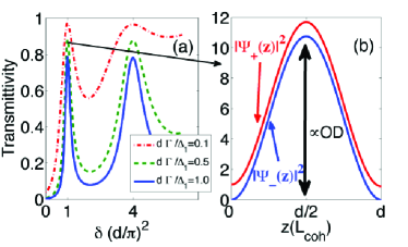
Figure 2: Linear case: (a) Transmittivtiy as a function of two-photon detuning. Transmission peaks are attenuated because of linear loss on $|a\rangle\rightarrow|b\rangle$ transition which are plotted for three different loss rates $\beta=d~{}\Gamma/\Delta_{1}$. (b) When the system is tuned on a transmission resonance ($\sqrt{\delta_{0}}d=n\pi$), the field inside the medium is amplified.

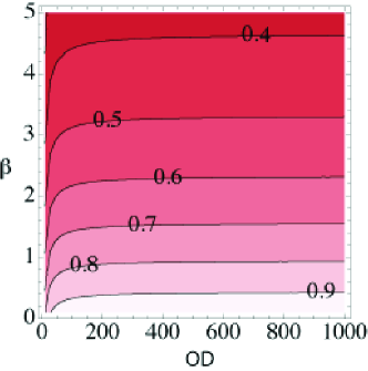
Figure 3: For large optical densities, the transmission on resonance ($\delta=\delta_{0}$), only depends on $\beta=OD\left(\frac{\Gamma}{\Delta_{1}|}\right)^{2}$.

The total number of polaritons in the system can be estimated by,

$$\mathcal{N}_{pol} = \int_{0}^{d}|\Phi_{+}(z)|^{2}+|\Phi_{-}(z)|^{2}dz$$

$$= \frac{(d^{2}+\pi^{2})^{2}}{4d\pi^{2}}|\Phi_{+}(0)|^{2}\simeq\frac{d^{3}}{4\pi^{2}}|\Phi_{+}(0)|^{2}.$$

This again shows that the polaritons experience many round trips inside the system before exiting. In particular, if we define the average intensity inside the medium as $|\Phi_{+}^{ave}|^{2}=\mathcal{N}_{pol}/d$, then we readily observe that the intensity of the polariton field is amplified inside the medium by the square of the system size $(|\Phi_{+}^{ave}|^{2}/|\Phi_{+}(0)|^{2}=(d/2\pi)^{2})$ – i.e. the finesse is proportional to the optical density (OD).

The original proposal for observing an enhanced Kerr nonlinearity with a four-level atomic system using EIT makes use of an optical cavity to enhance the nonlinearity Imamoglu et al. (1997). However, as pointed out in Ref. Grangier et al. (1998), the scheme suffers from some inaccuracies in the effective Hamiltonian. More specifically, in Ref. Imamoglu et al. (1997), the effective Hamiltonian was evaluated at the center of the EIT transparency window. However, in practice, EIT dramatically decreases the cavity linewidth because of the large dispersion that accompanies the vanishing absorption Lukin et al. (1998); this causes photons at frequencies slightly shifted from the central frequency to be switched out of the cavity. This leads to an extremely small allowable bandwidth for the incoming photons Grangier et al. (1998) and was neglected in the original analysis. We emphasize that the analysis presented here takes into account the dispersive properties of the medium, as we have included the field dynamics up to second order in the detuning from resonance (this accounts for the effective mass of the photons in our system). We verify the consistency of this derivation in Appendix A by solving the linear system including full susceptibilities. It is shown that the results are consistent near the two-photon resonance (i.e., frequencies around $\delta=0$).

IV Semi-classical nonlinear case

IV.1 Dispersive regime

In this section, in contrast to the previous section, we include the nonlinear term in the evolution equations to investigate its effect in the semi-classical limit (where the fields are still treated as complex numbers). In this picture, the effect of nonlinearity causes the transmission peaks to shift in frequency in an intensity-dependent way to the left or right depending on the sign of the nonlinearity coefficient $\kappa$. We show that when $|\kappa|OD\gg 1$, the magnitude of the shift is large even at intensities corresponding to that of a single photon. In this regime, we expect that the system can act as a single-photon switch and that signatures of quantum transport will become apparent (the quantum treatment is described in Sec.V).

Because of the self-phase modulation term in the evolution equations (Eqs. 12), the forward and backward fields acquire a phase shift proportional to their intensity. Moreover, due to the conjugate-phase modulation terms, each field undergo an extra phase shift proportional the intensity of the other field. Classically, this yields a frequency shift in the transmission spectrum when the nonlinearity is small. The shift in the transmission peak can be approximated by $\Delta\delta\simeq 2\kappa|\Phi_{+}^{ave}|^{2}$ where $|\Phi_{+}^{ave}|^{2}\simeq\frac{d^{2}}{4\pi^{2}}|\Phi_{+}(0)|^{2}$ is the average intensity of polaritons in the system. Suppose that we want the nonlinearity to be strong enough to shift the transmission peaks at least by half of their widths, $\Delta\delta\simeq\frac{1}{2}\delta^{3/2}$. Then, from Eq.(19) this condition can be written as

$$|\Phi_{+}^{{\rm{cr}}}(0)|^{2}=\left(\frac{\pi}{d}\right)^{5}\frac{1}{|\kappa|}$$ (21)

On the other hand, according to Eq.(III), we can write this condition in terms of the critical number of polaritons inside the system,

$$\mathcal{N}_{pol}^{{\rm{cr}}}=\frac{\pi^{3}}{4d^{2}\kappa}.$$ (22)

Since the nonlinearity coefficient is given by the light shift on the $|c\rangle\rightarrow|d\rangle$ transition, in the dispersive regime ($\Delta_{2}\gg\Gamma$), we have $\kappa=\frac{1}{4}\frac{\Gamma_{1D}}{\Gamma}\frac{\Gamma}{\Delta_{2}}$. Thus, we expect to have substantial nonlinearities at the level of one polariton (i.e., one incoming photon), $\mathcal{N}_{pol.}^{{\rm{cr.}}}=1$, if

$$d^{2}=\pi^{3}\frac{\Gamma}{\Gamma_{1D}}\frac{\Delta_{2}}{\Gamma}$$ (23)

where $\Gamma_{1D}$ is the rate of spontaneous emission rate into the guided modes. Strictly speaking, note that a single photon cannot actually have a nonlinear phase shift (as correctly derived later using a fully quantum picture); however, we can still use the results of this semiclassical calculation to qualitatively understand the relevant physics.

We can also rewrite the above condition in term of the optical density $(OD=d\frac{\Delta_{1}}{\Gamma})$ needed in the system. From the linear case, we know that an optimal detuning, for a transmission of 90%, should satisfy $d\frac{\Gamma}{\Delta_{1}}\sim 0.5$. Then, Eq. (23) can be written as

$$OD=2\pi^{3}\frac{\Gamma}{\Gamma_{1D}}\frac{\Delta_{2}}{\Gamma}.$$ (24)

Taking for example a system where $\Delta_{2}\sim 5\Gamma$ and $\frac{\Gamma_{1D}}{\Gamma}\sim 0.1$, nonlinearities at a few-photon level can be observed for an optical density ${\rm{OD}\simeq 6200}$.

First, let us consider the case of positive $\kappa$. In Fig. 4, we observe that at large enough optical density, the system can have very different transmission spectra for low and high intensities that classically correspond to having one and two polaritons (photons) inside the system, respectively. Although we have ignored the quantization of photons in this section, we can develop some insight into the transmission properties of one- and two-photon states. Loosely speaking, if we fix the input field frequency to lie at the one-photon (linear) transmission peak ($\delta_{0}$), the system would block the transmission of incident two-photon states. More realistically, suppose we drive the system with a weak classical field (coherent state), which can be well-approximated as containing only zero, one, and two-photon components. We then expect that the one-photon component will be transmitted through the system, while the two-photon component will be reflected, leading to anti-bunching of the transmitted light. We note that the general spirit of this conclusion is sound; however, the correct description of the system is achieved by taking into account the quantization of photons which is presented in the next sections.

A similar analysis holds for the case of negative $\kappa$. Note that the sign of $\kappa$ depends on the detuning of the photonic field from the atomic transition $|c\rangle\rightarrow|d\rangle$, which can easily be adjusted in an experiment. This is in contrast to conventional nonlinear optical fibers and nonlinear crystals, where the nonlinearity coefficient is fixed both in magnitude and sign. We find that a negative nonlinearity simply shifts the transmission spectrum in the opposite direction as for the positive case, as shown in Fig. 5, but all other conclusions remain the same. In particular, we would expect anti-bunching to occur for this case as well, when a weak coherent field is incident with its frequency fixed to the linear transmission resonance. Surprisingly, the quantum treatment (Sec.VII), shows that the above conclusion is wrong and system behaves very differently for negative nonlinearity. We show that this difference in behavior can be attributed to the presence of additional eigenstates (photonic bound states) in the medium and their excitation by the incident field.

For even larger nonlinearities or intensities, the transmission spectrum can become even more skewed and exhibit bistable behavior, as similarly found in Ref. Rapedius and Korsch (2008) in the context of transport of Bose-Einstein condensates in one dimension. There, the classical NLSE (Gross-Pitaevskii equation) was solved to find the mean-field transport properties of a condensate scattering off a potential barrier.

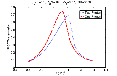
Figure 4: Due to nonlinearity, in the perturbative limit, the transmission spectrum shifts for different intensities. The integrated intensities inside the system is related to the number of present field quanta. OD=3000

Figure 5: For positive (negative) nonlinearity, in the perturbative limit, the transmission spectrum shifts to the right (left) of linear transmission spectrum (solid line), which is shown in dotted line (dashed line). The incoming intensity corresponds to one-photon in the system.

Instead of considering the switching effect as a function of number of photons inside the medium, we can also consider the number of photons that need to be sent into the system. Clearly, to have a well-defined transmission amplitude without substantial pulse distortion, the incident pulse must be long enough so that it fits within the bandwidth of the system resonance, as given in Eq. (19). To be specific, we consider an input pulse whose duration is equal to the inverse of the bandwidth, $t_{b}=(\frac{d}{\pi})^{3}t_{coh}$. We can relate the number of incoming photons to an average incident intensity:

$$|\Phi_{+}(0)|^{2}=\mathcal{N}_{pol.}\frac{t_{b}}{t_{coh}}=\frac{\mathcal{N}_{pol.}}{(d/\pi)^{3}}$$ (25)

Now, since the number of incident photons and incoming polaritons are the same, we can assign an average amplitude to any incoming photons number by Eq. (25), and evaluate the transmission. Hence, we can evaluate the number of incident photons needed to observe a significant nonlinearity and saturate the system. Fig. 6 shows the transmittivity of the nonlinear system as a function of number of photons in the incoming wavepacket. We observe that for high optical densities ($OD>1000$), the transmittivity drops as the number of incoming photons increases and the system gets saturated for even few photons.

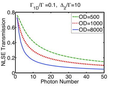
Figure 6: Transmission vs. the number of incident photons. For each OD, $\Gamma/\Delta_{1}$ is chosen so that the system exhibit a similar transmission for one photon.

IV.2 Dissipative Regime

In this section, we investigate the system in the presence of nonlinear absorption, where $\kappa$ is imaginary. The nonlinear dispersion of the previous case can simply be turned into nonlinear absorption by setting the nonlinear detuning to zero ($\Delta_{2}=0,~{}\kappa=\frac{\Gamma_{1D}}{2i\Gamma}$). In the quantum picture, this term does not affect the one-photon state, while two-photon states can be absorbed by experiencing three atomic transitions, $|a\rangle\rightarrow|b\rangle\rightarrow|c\rightarrow|d\rangle$, and subsequently being scattered from excited state $|d\rangle$ Harris and Yamamoto (1998). We consider the quantum treatment of absorption later and first study the semiclassical limit here.

The presence of nonlinear absorption suppresses the transmission of multi-photon states through the medium by causing them to decay. This suppression becomes stronger for higher intensities as shown in Fig. 7. We have used the same optical density (OD) and 1D confinement ($\Gamma_{1D}/\Gamma$) as in Fig. 4. We observe that the effects of nonlinear absorption are stronger than that of nonlinear dispersion studied in Sec.IV.1, since it occurs at resonance ($\Delta_{2}=0$) where the atomic response is strongest. It is thus possible to observe its effect at even lower intensities, corresponding to effective photon numbers two orders of magnitude smaller than the dispersive case. Much like the dispersive case, the suppression of transmission of multi-photon components should yield anti-bunching in the transmitted field. In this case, however, these components are simply lost from the system (as opposed to showing up as a bunched reflected field).

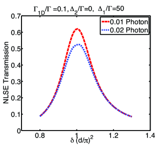
Figure 7: Due to nonlinear absorption, the transmission is suppressed for higher intensities. The integrated intensities inside the system is related to the number of present field quanta. OD=3000

V Quantum nonlinear formalism: Few-photon limit

In this section, we describe a quantum mechanical approach that enables one to solve the problem of quantum transport of a small number of photons through the finite, nonlinear system described in Sec.II. This few-photon number limit is of particular interest since it captures the physics of single-photon switching.

We find it convenient to study the dynamics of the system of photons in the Schrödinger picture, where one can explicitly solve for the few-body wave functions. This approach is made possible by truncating the Hilbert space so that only subspaces with $n_{max}$ photons are less are present. In the following, we will consider the case where $n_{max}=2$, although our analysis can be easily extended to cover any other value. This truncation is justified when the incident coherent field is sufficiently weak that the average photon number is much smaller than one inside the system ($|\alpha_{0}|^{2}d^{3}\ll 1$, where $\alpha_{0}$ is the amplitude of the incoming field). Thus, we can write the general state of the system as:

$$|\psi(t)\rangle \simeq \int dz_{1}dz_{2}\phi(z_{1},z_{2},t)S^{\dagger}(z_{1})S^{\dagger}(z_{2})|0\rangle$$

$$+ \int dz\theta(z,t)S^{\dagger}(z)|0\rangle+\epsilon|0\rangle.$$

The first, the second and the third term correspond to two-photon, one-photon and vacuum state, respectively. Note that because of bosonic symmetrization, $\phi(z_{1},z_{2},t)$ should be symmetric in $z_{1}$ and $z_{2}$. This formalism allows us to capture any non-trivial spatial order between photons in our system (e.g., the de-localization of two photons as represented by the off-diagonal terms in $\phi(z_{1},z_{2})$). Since the NLSE Hamiltonian commutes with the field number operator $\hat{S}^{\dagger}\hat{S}$, manifolds with different field quanta are decoupled from each other inside the medium. Therefore, the evolution for the one-photon and two-photon manifolds under the NLSE Hamiltonian can be written as,

$$i\frac{\partial}{\partial t}\phi(z_{1},z_{2},t) = -\frac{1}{2m}\left(\frac{\partial^{2}}{\partial z_{1}^{2}}+\frac{\partial^{2}}{\partial z_{2}^{2}}\right)\phi(z_{1},z_{2},t)$$ (27)

$$+ 2\kappa\phi(z_{1},z_{2},t)\delta(z_{1}-z_{2})$$

$$i\frac{\partial}{\partial t}\theta(z,t)=-\frac{1}{2m}\frac{\partial^{2}}{\partial z^{2}}\theta(z,t).$$ (28)

However, the system is driven with an input field at $z=0$, which allows different manifolds to be coupled at the boundaries. This is analogous to fiber soliton experiments where a classical input field mixes quantum solitons with different photon numbers Drummond et al. (1993); Haus (2000); Agrawal (2007). In particular, for a classical input field,

$$\hat{\Psi}_{+}(z=0)|\psi(t)\rangle = \alpha(t)|\psi(t)\rangle$$ (29)

$$\hat{\Psi}_{-}(z=d)|\psi(t)\rangle = 0|\psi(t)\rangle,$$ (30)

which corresponds to a coherent state with (possibly time-dependent) amplitude $\alpha(t)$ as an input at $z=0$, and no input (i.e., vacuum) at $z=d$. Since we specify that the input coherent field is weak ($\alpha\ll 1$), the amplitude of the vacuum state is almost equal to one ($\epsilon\simeq 1$). The annihilation operator in these equations reduces the photon number on the left-hand side by one. Thus, such boundary conditions relate different photon subspaces whose photon number differ by one, e.g. the two-photon and one-photon wavefunctions. In the adiabatic limit where the anti-symmetric part of the field ($A=(\hat{\Psi}_{+}-\hat{\Psi}_{-})/\sqrt{2}$) follows the symmetric part ($S=(\hat{\Psi}_{+}+\hat{\Psi}_{-})/\sqrt{2}$), we have

$$\Psi_{+}=\frac{1}{\sqrt{2}}(S-\frac{i}{2m}\partial_{z}S)~{}~{}~{},~{}~{}~{}\Psi_{-}=\frac{1}{\sqrt{2}}(S+\frac{i}{2m}\partial_{z}S).$$ (31)

Therefore the boundary conditions at $z=0$ can be re-written as

$$\frac{1}{\sqrt{2}} \int dz_{1}dz_{2}~{}[S-\frac{i}{2m}\partial_{z}S]_{z=0}S^{\dagger}(z_{1})S^{\dagger}(z_{2})\phi(z_{1},z_{2},t)|0\rangle$$

$$= \alpha\int dz\theta(z,t)S^{\dagger}|0\rangle,$$

$$\frac{1}{\sqrt{2}} \int dz~{}[S-\frac{i}{2m}\partial_{z}S]_{z=0}S^{\dagger}(z)\theta(z,t)|0\rangle=\alpha|0\rangle.$$

Using the identity $\int[\partial_{z}S(z),S^{\dagger}(z^{\prime})]f(z^{\prime})dz^{\prime}=\partial_{z}f(z)$, the boundary conditions on the one-photon and two-photon wave functions can be written as:

$$\phi(z_{1}=0,z_{2},t)-\frac{i}{2m}\partial^{(1)}\phi(z_{1},z_{2},t)|_{z_{1}=0} = \frac{\alpha}{\sqrt{2}}\theta(z_{2},t)$$

$$\theta(z=0,t)-\frac{i}{2m}\partial_{z}\theta(z=0,t) = \sqrt{2}\alpha,$$ (33)

where $\partial^{(1)}$ acts on the first parameter. This type of open boundary condition is known as a Robin or mixed boundary condition, which involves a combination of both the function and its derivative. In the present case, the open boundary conditions allow particles to freely enter and leave the system. We emphasize that this process is noise-less, in that the loss of population from the interior of our system is related by our boundary condition equations to the flow of particle current through the system boundaries. This is in contrast to an optical cavity, for instance, where photons inside the cavity leak dissipatively into the environment Gardiner and Collett (1985). Similarly the boundary condition at $z=d$ reads

$$\phi(d,z,t)+\frac{i}{2m}\partial^{(1)}\phi(d,z,t) = 0$$ (34)

$$\theta(d,t)+\frac{i}{2m}\partial_{z}\theta(d,t) = 0.$$ (35)

Given the boundary conditions and the equations of motion in the interior, we can completely solve for the photon wavefunctions.

Once the wavefunctions are determined, it is possible to determine the intensity profile as well as any other correlation function for the photons. For example, the intensity of the forward-going polariton is

$$I(z,t) = \langle\psi(t)|\hat{\Psi}_{+}^{\dagger}(z)\hat{\Psi}_{+}(z)|\psi(t)\rangle$$

$$= \langle 1|\hat{\Psi}_{+}^{\dagger}(z)\hat{\Psi}_{+}(z)|1\rangle+\langle 2|\hat{\Psi}_{+}^{\dagger}(z)\hat{\Psi}_{+}(z)|2\rangle,$$

where $|j\rangle$ denotes the component of the total wavefunction $|{\psi(t)}\rangle$ containing $j$ photons. The first and second terms on the right thus correspond to the one- and two-photon contributions to the intensity. By re-writing expressions in terms of $S$ instead of $(\hat{\Psi}_{+},\hat{\Psi}_{-})$, we obtain:

$$I(z,t) = \frac{1}{2}\left|\theta(z)-\frac{i}{2m}\partial_{z}\theta(z)\right|^{2}$$

$$+ 2\int dz^{\prime}\left|\phi(z^{\prime},z)-\frac{i}{2m}\partial^{(2)}\phi(z^{\prime},z)\right|^{2}$$

Similarly, the second-order correlation function for the forward field is

$$\langle\psi|\hat{\Psi}_{+}^{\dagger 2}(z)\hat{\Psi}_{+}^{2}(z)|\psi\rangle=$$

$$\left|\phi(z,z)-\frac{i}{m}\partial^{(1)}\phi(z,z)-\frac{1}{4m^{2}}\partial^{(1)}\partial^{(2)}\phi(z,z)\right|^{2}$$

which in our truncated space only depends on the two-photon wave function. Now, we evaluate the normalized second-order correlation function $g_{2}(z)$, which characterizes the photon statistics of an arbitrary field. This function takes the form

$$g_{2}(z)=\frac{\langle\psi|\hat{\Psi}_{+}^{\dagger 2}(z)\hat{\Psi}_{+}^{2}(z)|\psi\rangle}{\left|\langle\psi|\hat{\Psi}_{+}^{\dagger}(z)\hat{\Psi}_{+}(z)|\psi\rangle\right|^{2}},$$ (39)

and physically characterizes the relative probability of detecting two consecutive photons at the same position $z$. If this quantity is less (greater) than one, the photonic field is anti-bunched (bunched). In particular, if $g_{2}(z)=0$, the field is perfectly anti-bunched and there is no probability for two photons to overlap in position. In our truncated Hilbert space, $g_{2}(z)$ of the transmitted field is given by

$$g_{2}(z=d)\simeq\frac{\langle 2|\Psi_{+}^{\dagger 2}(d)\Psi_{+}^{2}(d)|2\rangle}{\left|\langle 1|\Psi_{+}^{\dagger}(d)\Psi_{+}(d)|1\rangle+\langle 2|\Psi_{+}^{\dagger}(d)\Psi_{+}(d)|2\rangle\right|^{2}}$$ (40)

We note that this expression can be simplified, since at $z=d$, we have $\Psi_{-}=\frac{1}{\sqrt{2}}(S+\frac{i}{2m}\partial_{z}S)=0$ and $\Psi_{+}=\sqrt{2}S$. Therefore,

$$g_{2}(d)=\frac{4|\phi(d,d)|^{2}}{\left(\left|\theta(d)\right|^{2}+4\int dz^{\prime}\left|\phi(z^{\prime},d)\right|^{2}\right)^{2}}.$$ (41)

We can also evaluate the stationary two-time correlation, which is defined in the Heisenberg picture as:

$$g_{2}(z,\tau)=\frac{\langle\psi|\Psi_{+}^{\dagger}(z,0)\Psi_{+}^{\dagger}(z,\tau)\Psi_{+}(z,\tau)\Psi_{+}(z,0)|\psi\rangle}{\left|\langle\psi|\Psi_{+}^{\dagger}(z,0)\Psi_{+}(z,0)|\psi\rangle\right|^{2}},$$ (42)

where the denominator is simplified in the stationary steady-state regime. This correlation function characterizes the probability of detecting two photons at position $z$ but separated by time $\tau$. We can re-write $g_{2}(z,\tau)$ in terms of wavefunctions in the Schrödinger picture in the following way. We first note that the expression $|\tilde{\psi}(0)\rangle=\hat{\Psi}_{+}(z,0)|\psi\rangle$ appearing in the equation above can be thought of as a new wavefunction, which describes the state of the system after a photon is initially detected at time $t=0$ and position $z$. This new state naturally has one less photon than the original state, and by simplifying the expressions, it can be written as:

$$|\tilde{\psi}(0)\rangle=\int\theta^{{\rm{new}}}(z^{\prime})S^{\dagger}(z^{\prime})|0\rangle+\epsilon^{{\rm{new}}}|0\rangle$$ (43)

where the new one-photon and vacuum amplitudes are given by

$$\frac{\theta^{{\rm{new}}}}{\sqrt{2}} = \phi(d,z^{\prime},t=0)-\frac{i}{2m}\partial^{(1)}\phi(d,z^{\prime},t=0)$$ (44)

$$\epsilon^{{\rm{new}}} = \frac{1}{\sqrt{2}}\left(\theta(d,t=0)-i\partial\theta(d,t=0)\right).$$ (45)

Here we have assumed that $z=d$, since we are interested in the transmitted field. Now, Eq. (42) can be written as

$$g_{2}(d,\tau)=\langle\tilde{\psi}(0)|\hat{\Psi}_{+}^{\dagger}(d,\tau)\hat{\Psi}_{+}(d,\tau)|\tilde{\psi}(0)\rangle/|\langle\tilde{\psi}(0)|\tilde{\psi}(0)\rangle|^{2}.$$ (46)

The numerator describes the expectation value for the intensity operator $\hat{I}(\tau)=\hat{\Psi}_{+}^{\dagger}(d,\tau)\hat{\Psi}_{+}(d,\tau)$ in the Heisenberg picture given an initial state $|\tilde{\psi}(0)\rangle$. However, we can easily convert this to the Schrödinger picture by moving the evolution from the operator to the state, i.e., by evolving $|\tilde{\psi}(0)\rangle$ under the same evolution equations (Eqs. 27-28) and boundary conditions (Eq. 33) that we used earlier. Therefore, the correlation function $g_{2}(z,\tau)$ will be given by:

$$g_{2}(z,\tau)=\frac{\langle\tilde{\psi}(\tau)|\Psi_{+}^{\dagger}(z)\Psi_{+}(z)|\tilde{\psi}(\tau)\rangle}{\left|\langle\psi(0)|\Psi_{+}^{\dagger}(z)\Psi_{+}(z)|\psi(0)\rangle\right|^{2}}.$$ (47)

VI Analytical solution for NLSE with open boundaries

In this section, we show that a NLSE system with open boundary conditions yields analytical solutions in absence of an outside driving source ($\alpha_{0}=0$). To obtain the analytical solutions, we use the Bethe ansatz technique Lieb and Liniger (1963); Lai and Haus (1989b). This ansatz specifies that the eigenstates consist of a superposition of states in which colliding particles exchange their wavenumbers $k_{i}$. Unlike the typical formulation, the values of $k_{i}$ here can be complex to reflect the open nature of our boundary conditions, which allow particles to freely enter or leave. In particular, we present the one-, two- and many-body eigenmodes of the system along with their energy spectra. Finding certain eigenmodes of the system (e.g., bound states) helps us understand the correlation functions and also spatial wavefunctions which are numerically calculated later in Sec.VII for a driven system.

VI.1 One-particle problem

First, we calculate the fundamental modes for the one-particle states. These modes are of particular interest when we later want to construct the many-body wavefunction of the interacting system in the absence of an input field.

Specifically, we want to find solutions of the Schrödinger equation for a single particle in a system of length $d$,

$$i\frac{\partial}{\partial t}\theta(z,t)=-\frac{1}{2m}\frac{\partial^{2}}{\partial z^{2}}\theta(z,t),$$ (48)

subject to open boundary conditions. The boundary condition for the undriven system at $z=0$ is given by

$$\theta(0)-\frac{i}{2m}\partial_{z}\theta(0)=0$$ (49)

and similarly for $z=d$,

$$\theta(d)+\frac{i}{2m}\partial_{z}\theta(d)=0.$$ (50)

We look for stationary solutions of the form $\theta(z,t)=e^{-i\delta t}\theta(z)$, where $\theta(z)=A\sin(kz)+B\cos(kz)$. For simplicity, we assume $m=1/2.$ Therefore, we recover the quadratic dispersion relation $\delta=k^{2}$. The values of $k$ are allowed to be complex to reflect the open nature of our boundary conditions, which allows particles to freely enter or leave. By enforcing the boundary conditions we get a set of equations for the coefficients $A,B$,

$$B-iAk=0,$$

$$(A-iBk)\sin(kd)+(B+iAk)\cos(kd)=0,$$

which yields the characteristic equation for finding eigenmodes and eigen-energies of system,

$$e^{2ikd}=\left(\frac{k+1}{k-1}\right)^{2}.$$ (51)

Therefore the normalized corresponding wave function for each allowed k will be:

$$\theta(z) = A(\sin(kz)+ik\cos(kz)),$$ (52)

$$A^{2} = \frac{4k}{2dk(1+k^{2})+(k^{2}-1)\sin(2dk)}$$

We note that in the limit of large optical density $d\gg 1$, the lowest energy modes of the open system are very close to those of a system with closed boundary conditions, whose characteristic equation is given by $kd=n\pi$. For example, at $d=100$, the wave number corresponding to lowest energy is $k{\simeq}0.0314-i0.00063\simeq\pi/100$. We note that the many-body solutions of the system in the presence of very strong interactions (large $\kappa$) can be constructed from these single-particle solutions and proper symmetrization, as we show in Sec.VI.5.

VI.2 Two-particle problem

In this section, we study the problem of two particles obeying the NLSE with mixed boundary conditions. We wish to solve

$$E\phi(z_{1},z_{2}) = -\frac{1}{2m}\left(\frac{\partial^{2}}{\partial z_{1}^{2}}+\frac{\partial^{2}}{\partial z_{2}^{2}}\right)\phi(z_{1},z_{2})$$ (53)

$$+ 2\kappa\phi(z_{1},z_{2})\delta(z_{1}-z_{2}),$$

where $E$ is the energy of the system and can be complex. Again, we assume the mass is entirely real, $m=1/2$.

We should note that the conventional method of separation of variables cannot be applied in this case. The reason for this can be understood in the following way. On one hand, if we ignore the delta interaction term in the evolution equation of the two particles, finding the eigenfunctions is essentially equivalent to solving the Laplace equation in a box with mixed boundary conditions. Therefore, for this problem the natural separation of variables involves solutions given by products of functions $f(z_{1})$ and $g(z_{2})$. On the other hand, if we neglect the boundaries, the problem of two particles interacting at short range can be solved by utilizing the center of mass and relative coordinates and invoking solutions involving products of functions $\tilde{f}(z_{1}+z_{2})$ and $\tilde{g}(z_{1}-z_{2})$. We immediately see that the two sets of solutions are irreconcilable and thus separation of variables is not applicable when both the boundary conditions and interaction term are present.

We thus take a different approach, using a method similar to the Bethe ansatz method for continuous, one-dimensional systems Lieb and Liniger (1963). Specifically, we solve the Schrödinger equation in the triangular region where $0\leq z_{1}<z_{2}\leq d$, and we treat the interaction as a boundary condition at $z_{1}=z_{2}$. In other words, when two particles collide with each other at $z_{1}=z_{2}$, they can exchange momenta, which is manifested as a cusp in the wave function at $z_{1}=z_{2}$. Hence, for the boundary conditions in this triangular region, we have

$$\phi(0,z_{2})-i\partial_{z_{1}}\phi(0,z_{2}) = 0$$ (54)

$$\phi(z_{1},d)+i\partial_{z_{2}}\phi(z_{1},d) = 0$$ (55)

$$\left(\partial_{z_{2}}-\partial_{z_{1}}\right)\phi(z_{1},z_{2})|_{z_{2}=z_{1}} = \kappa\phi(z_{1},z_{2})|_{z_{2}=z_{1}}$$ (56)

We note that the last boundary condition is deduced from integrating Eq. (53) across $z_{1}=z_{2}$ and enforcing that the wavefunction is symmetric,

$$\left(\partial_{z_{2}}-\partial_{z_{1}}\right)\phi(z_{1},z_{2})|_{z_{2}=z_{1}^{+}} - \left(\partial_{z_{2}}-\partial_{z_{1}}\right)\phi(z_{1},z_{2})|_{z_{2}=z_{1}^{-}}$$ (57)

$$= 2\kappa\phi(z_{1},z_{2})|_{z_{1}=z_{2}}.$$

Inside the triangle, the solution consists of superpositions of free particles with complex momenta. Since particles can exchange momenta when they collide at $z_{1}=z_{2}$, we should consider solutions of the following form,

$$\phi(z_{1},z_{2})=\sum_{\{\epsilon\}}\mathcal{A}_{\epsilon}e^{i\epsilon_{1}k_{1}z_{1}+i\epsilon_{2}k_{2}z_{2}}+\mathcal{B}_{\epsilon}e^{i\epsilon_{1}k_{2}z_{1}+i\epsilon_{2}k_{1}z_{2}}$$ (58)

where the summation should be performed on all sets of signs $\epsilon=\pm 1$. Given the terms containing $\mathcal{A}_{\epsilon}$, the terms $\mathcal{B}_{\epsilon}$ then arise from the scattering of the particles off each other. Let’s first consider the portion of the wavefunction containing the terms $\mathcal{A}_{\epsilon}$, which we can write in the form:

$$\phi_{\mathcal{A}}(z_{1},z_{2}) = e^{ik_{1}z_{1}+ik_{2}z_{2}}+\alpha e^{-ik_{1}z_{1}+ik_{2}z_{2}}$$

$$+ \beta e^{-ik_{1}z_{1}-ik_{2}z_{2}}+\gamma e^{+ik_{1}z_{1}-ik_{2}z_{2}},$$

where the energy is equal to $E=k_{1}^{2}+k_{2}^{2}$ and could be complex. Similar to the single-particle solutions, the presence of the imaginary part in the energy reflects the fact that the two-particle state stays a finite amount of time inside the system. Applying boundary conditions at $z=0$ and $z=d$ subsequently generates four equations relating $\alpha,\beta,\gamma$ where one of them is redundant. Their solution reduces the wavefunction to

$$\phi_{\mathcal{A}}(z_{1},z_{2}) = e^{ik_{1}z_{1}+ik_{2}z_{2}}+\frac{k_{1}+1}{k_{1}-1}e^{-ik_{1}z_{1}+ik_{2}z_{2}}$$

$$+ \frac{k_{1}+1}{k_{1}-1}\gamma e^{-ik_{1}z_{1}-ik_{2}z_{2}}+\gamma e^{+ik_{1}z_{1}-ik_{2}z_{2}}$$

where $\gamma=\frac{k_{2}-1}{k_{2}+1}e^{2ik_{2}d}$. A similar expression results for the portion of $\phi(z_{1},z_{2})$ containing the $\mathcal{B}_{\epsilon}$ terms, once the boundary conditions at $z=0$ and $z=d$ are applied:

$$\phi_{\mathcal{B}}(z_{1},z_{2}) = \frac{1}{t}\left(e^{ik_{2}z_{1}+ik_{1}z_{2}}+\frac{k_{2}+1}{k_{2}-1}e^{-ik_{2}z_{1}+ik_{1}z_{2}}\right)$$

$$+ \frac{\gamma^{\prime}}{t}\left(\frac{k_{2}+1}{k_{2}-1}e^{-ik_{2}z_{1}-ik_{1}z_{2}}+e^{+ik_{2}z_{1}-ik_{1}z_{2}}\right)$$

where $\gamma^{\prime}=\frac{k_{1}-1}{k_{1}+1}e^{2ik_{1}d}$, and $t$ is a coefficient to be determined from the boundary condition at $z_{1}=z_{2}$. To find $t$, it is convenient to re-write each of ther terms in $\phi_{\mathcal{A,B}}$ as a product of relative coordinate ($r=z_{2}-z_{1}$) and center-of-mass coordinate ($R=(z_{1}+z_{2})/2$) functions,

$$\tilde{\phi}_{\mathcal{A}}(R,r) = e^{ipR-iqr}+\frac{k_{1}+1}{k_{1}-1}e^{-iqR+ipr}$$ (61)

$$+ \gamma\frac{k_{1}+1}{k_{1}-1}e^{-ipR+iqr}+\gamma e^{iqR-ipr},$$ (62)

$$\tilde{\phi}_{\mathcal{B}}(R,r) = \frac{1}{t}(e^{ipR+iqr}+\frac{k_{2}+1}{k_{2}-1}e^{iqR+ipr}$$ (63)

$$+ \gamma^{\prime}\frac{k_{2}+1}{k_{2}-1}e^{-ipR-iqr}+\gamma^{\prime}e^{-iqR-ipr}),$$ (64)

where $p=(k_{1}+k_{2})$ and $q=(k_{1}-k_{2})/2$. The boundary condition at $z_{1}=z_{2}$ leaves the center-of-mass parts of the wavefunction unaffected, but yields the following condition on the relative coordinates,

$$\partial_{r}\phi(R,r)|_{r=0^{+}}=\frac{\kappa}{\sqrt{2}}\phi(R,r)|_{r=0^{+}}.$$ (65)

where $\phi=\phi_{\mathcal{A}}+\phi_{\mathcal{B}}$ is the total wavefunction in the triangular region. We should satisfy this boundary condition separately for each of the center-of-mass momentum terms $e^{{\pm}ipR},e^{{\pm}iqR}$ in the total wavefunction. This leads to three independent equations (one out of four is redundant). However, we introduce a new parameter ($t^{\prime}$) to simplify the equations, which turns them into four equations:

$$t=\frac{k_{1}-k_{2}+i\kappa}{k_{1}-k_{2}-i\kappa}~{}~{} ~{}~{}t^{\prime}=\frac{k_{1}+k_{2}+i\kappa}{k_{1}+k_{2}-i\kappa}$$ , (66)

$$t~{}t^{\prime}\left(\frac{k_{1}+1}{k_{1}-1}\right)^{2} = e^{2ik_{1}d}$$ (67)

$$t^{\prime}\left(\frac{k_{2}+1}{k_{2}-1}\right)^{2} = te^{2ik_{2}d},$$ (68)

which can be written in the following short form:

$$e^{2ik_{i}d}=\frac{(k_{i}+1)^{2}}{(k_{i}-1)^{2}}\prod_{j\neq i}\frac{(k_{i}-k_{j}+i\kappa)(k_{i}+k_{j}+i\kappa)}{(k_{i}-k_{j}-i\kappa)(k_{i}+k_{j}-i\kappa)}$$ (69)

where $i,j$ can be (1,2). These are transcendental equations for ($k_{1},k_{2}$), which generate the spectrum of two interacting particles. We can also write the wave functions ($\phi=\phi_{\mathcal{A}}(z_{1},z_{2})+\phi_{\mathcal{B}}(z_{1},z_{2})$) in the region ($0\leq z_{1}<z_{2}\leq d)$ in a more compact way, by using the single particle solutions $\eta_{k}(z)=\sin(kz)+ik\cos(kz)$:

$$\phi_{\mathcal{A}}(z_{1},z_{2}) = \frac{4}{k_{1}-1}\frac{e^{ik_{2}d}}{k_{2}+1}\eta_{k_{1}}(z_{1})\eta_{k_{2}}(d-z_{2})$$ (70)

$$\phi_{\mathcal{B}}(z_{1},z_{2}) = \frac{4t^{-1}}{k_{2}-1}\frac{e^{ik_{1}d}}{k_{1}+1}\eta_{k_{2}}(z_{1})\eta_{k_{1}}(d-z_{2}).$$ (71)

It is interesting to note that in the limit of strong interaction (either for positive or negative $\kappa$), the solutions are very similar to the non-interacting case. The reason can be seen from the transcendental Eqs. (69), in the limit $\kappa\rightarrow\pm\infty$. We then recover the same characteristic equations $e^{2ikd}=(\frac{k+1}{k-1})^{2}$ for both wavevectors as the non-interacting case, Eq. (51). We should note that there are some trivial solutions to the transcendental Eqs. (69), which do not have any physical significance. For example, equal wave vectors $k_{1}=k_{2}$. Although one can find such wave vectors, this solution is readily not a solution to Eq.(53), since it does not satisfy the interacting part (this solution only contains center of mass motion). One can also plug back the wave vectors into wave function and arrive at a wave function equal to zero everywhere. Another example is when one of the wave vectors is zero. In this case, one can also show that the wave function is zero everywhere. If $(k_{1},k_{2})$ are solutions to the transcendental equations, then $(\pm k_{1},\pm k_{2})$ are also solutions with equal energies. In next two sections, we investigate non-trivial solutions to the transcendental equation for two particles and discuss the related physics.

VI.3 Solutions close to non-interacting case

The transcendental equations allow a set of solutions with the wavevectors close to two different non-interacting modes say $(m,n)$. In the non-interacting regime, any mode can be populated by an arbitrary number of photons. However, once the interaction is present, photons can not occupy the same mode and therefore, the photons will reorganize themselves and each acquire different modes. Fig. 8 shows a normal mode wavefunction of a non-driven system in both non-interacting and strongly interacting regime ($\kappa d\gg 1$). The wave function has a cusp on its diagonal and diagonal elements are depleted for both repulsive and attractive strong interaction.

This is a manifestation of fermionization of bosons in one dimensional system in the presence of strong interaction Girardeau (1960); Lieb and Liniger (1963). Such solutions can exist both for repulsive and attractive interactions. However, we note in the case of attractive interaction such solutions are not the ground state of the system and solutions with lower energies exist which will be discussed below. We later argue that indeed on the repulsive side, the anti-bunching behavior of a driven system is due to the repulsion of the photons inside the medium. We can also estimate the energy of such modes which is always positive. In the strong interacting regime, particles avoid each other and therefore, their energy of a strongly two interacting bosons $E(m,n)$ will be equal to the energy of a system which has two non-interacting bosons, one in state $m$ and the other in state $n$. This is shown in Fig. 9, where by increasing the interaction strength the energy of interacting particles reaches that of the non-interacting particles. As we pointed out in the previous section (Sec.VI.1), the energy of modes ($E(n)$) in an open box has an imaginary part which represents how fast the particle leave the system. However, for large systems ($d\gg 1$), this decay is very small compared to the energy of the mode and one can approximate the energy of an open system by that of a closed box (i.e. $E(n)\simeq(\frac{n\pi}{d})^{2}$). Therefore, the energy of two strongly interacting photons ($\kappa d\gg 1$), in the limit of large system ($d\gg 1$), will be given by:

$$E(n,m)\simeq\left(\frac{n\pi}{d}\right)^{2}+\left(\frac{m\pi}{d}\right)^{2}$$ (72)

We note that our strongly interacting system is characterized by the parameter $\kappa d$ which is the same $\gamma$-parameter conventionally used for interacting 1D Bose gas. More precisely, the $\gamma$-parameter which is the ratio of the interaction to kinetic energy can be simplified in our case for two particles: $m\kappa d/2=\kappa d/4$.

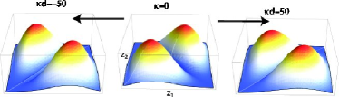
Figure 8: The amplitude of the two-photon wavefunction for (m=1, n=2) mode when the system is not driven. By increasing the interaction, photons self-organize inside the medium and exhibit anti-bunching (depletion of diagonal elements). For this plot: $d=30$.

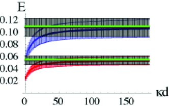
Figure 9: Energy of two-photon states: by increasing the interaction strength ($\kappa d\gg 1$) the energy of interacting particles (red:E(1,2) and blue:E(1,3)) reaches that of the non-interacting particles (black). For large system (in this case $d=30\gg 1$), the energy limit is equal to energy of particles in a closed box (green). The error bars show that imaginary part of the energies.

VI.4 Bound States Solution

For attractive interaction ($\kappa<0$), the mode equation (69) admits solutions which take the form of photonic bound states. Specifically, in the reference frame of the center of mass, two particles experience an attractive delta function interaction $-2|\kappa|\delta(z_{2}-z_{1})\rightarrow-\sqrt{2}|\kappa|\delta(r)$, which allows one bound state in the relative coordinate. Therefore, the part of the wavefunction describing the relative coordinate roughly takes the form $e^{iq|r|}$, where the relative momentum $q=(k_{1}-k_{2})/\sqrt{2}\simeq i|\kappa|/\sqrt{2}$ is imaginary and its energy is about $-\kappa^{2}/2$. On the other hand, the center of mass momentum can take a discrete set of values that are determined by the system boundary conditions. We find that the center of mass solutions can be approximately described by two different types. The first type is where the real part of each photon wavevector roughly takes values allowed for a single particle in a box, such that $k_{1}\simeq\left(\frac{n\pi}{d}\right)+i\frac{\kappa}{2}$ and $k_{2}\simeq\left(\frac{n\pi}{d}\right)-i\frac{\kappa}{2}$. In this case the center of mass has wavevector $p=k_{1}+k_{2}\simeq 2(\frac{n\pi}{d})$. The corresponding energies for these states are

$$E_{n}^{b}\simeq 2\left(\frac{n\pi}{d}\right)^{2}-\frac{\kappa^{2}}{2}.$$ (73)

Here, the first term on the right corresponds to the energy of the center of mass motion, and the second term corresponds to the bound-state energy of the relative motion. Fig. 12 shows that the energies estimated in this way agree very well with the exact values obtained by solving the transcendental Eqs. (69).

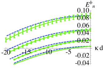
Figure 10: Energy of bound states versus strength of nonlinearity. Green (solid) curves are obtained by solving transcendental Eqs. (69). Blue (dashed) curves are estimated based on $E_{n}^{b}\simeq 2\left(\frac{n\pi}{d}\right)^{2}-\frac{\kappa^{2}}{2}$. In this plot $d=30$.

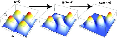
Figure 11: The amplitude of the two-photon wavefunction for a bound state when the system is not driven. By increasing interaction, photons becomes more bunched. $(k_{1},k_{2})\simeq\left(\frac{n\pi}{d}\right)\pm i\frac{\kappa}{2}$. For this plot: $d=60,n=3$.

The second type of solution allowed for the center of mass motion is where its energy approximately takes a single-particle value, $\frac{p^{2}}{2(2m)}=(\frac{n\pi}{d})^{2}$ where $p=k_{1}+k_{2}\simeq\sqrt{2}(\frac{n\pi}{d})$. Therefore, the momentum of individual particles will be given by $k_{1}\simeq\left(\frac{n\pi}{\sqrt{2}d}\right)+i\frac{\kappa}{2}$, $k_{2}\simeq\left(\frac{n\pi}{\sqrt{2}d}\right)-i\frac{\kappa}{2}$ and the energy of this paired composite can be estimated as

$$E_{n}^{b}\simeq\left(\frac{n\pi}{d}\right)^{2}-\frac{\kappa^{2}}{2}.$$ (74)

Again, the estimated energies agree well with exact solutions, as shown in Fig. 12. We note that some of the estimated allowed energies for the two types of center of mass solutions coincide (e.g., the lowest lying energy level in Fig. 10 and Fig. 12).

The energies of this series of bound states decrease with increasing strength of nonlinearity $|\kappa|$. Now, suppose we drive the system with a coherent field of fixed frequency $\delta$, while varying $\kappa$. The system is expected to display a set of resonances as $|\kappa|$ is increased, each time $\delta$ is equal to some particular bound state energy $E_{n}^{b}$. This effect in fact gives rise to oscillatory behavior in the correlation functions as a function of $\kappa$, as we will see later (Fig. 18(a) and (b)).

The wavefunction amplitude of a typical bound state is shown in Fig. 13. Due to the attractive interaction, diagonal elements $z_{1}=z_{2}$ become more prominent as $|\kappa|$ increases, indicating a stronger bunching effect for the photons, and these states become more tightly bound in the relative coordinate. The center of mass of the bound states can acquire a free momentum that is quantized due to the system boundary conditions (e.g., $k\simeq n\pi/d$). Fig. 13 shows the wavefunction of the third bound state (n=3). The three peaks evident for large $|\kappa|$ reflect the quantum number of the center of mass motion.

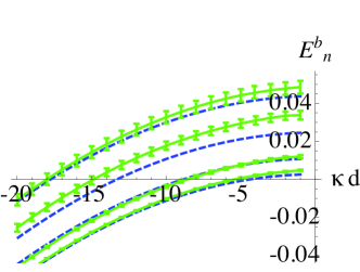
Figure 12: Energy of bound states versus strength of nonlinearity. Green (solid) curves are obtained by solving transcendental Eqs. (69). Blue (dashed) curve are estimated based on $E_{n}^{b}\simeq\left(\frac{n\pi}{d}\right)^{2}-\frac{\kappa^{2}}{2}$. In this plot $d=30$.

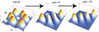
Figure 13: The amplitude of the two-photon wavefunction for a bound state for a non-driven system. By increasing interaction, photons becomes more bunched. $(k_{1},k_{2})\simeq\left(\frac{n\pi}{\sqrt{2}d}\right)\pm i\frac{\kappa}{2}$. For this plot: $d=60,n=3$.

VI.5 Many-body problem

In this section, we obtain the general solution for the many-body case. For the many-body system, the Schrödinger equation takes the form

$$E\phi(z_{1},...,z_{N}) = -\frac{1}{2m}\sum_{i}\frac{\partial^{2}}{\partial z_{i}^{2}}\phi(z_{1},...,z_{N})$$ (75)

$$+ \sum_{<i,j>}2\kappa\phi(z_{1},...,z_{N})\delta(z_{i}-z_{j}),$$ (76)

where $<i,j>$ indicates pairs of particles. The open boundary conditions for the many-body problem are given by

$$\left[\phi(z_{1},...,z_{N})-i\frac{\partial}{\partial z_{i}}\phi(z_{1},...,z_{N})\right]_{z_{i}=0} = 0$$ (77)

$$\left[\phi(z_{1},...,z_{N})+i\frac{\partial}{\partial z_{i}}\phi(z_{1},..,z_{N})\right]_{z_{i}=d} = 0.$$ (78)

Before presenting the general many-body solution, we first study the limit of very large interaction strength for two particles. In the limit of hardcore bosons where $\kappa\rightarrow\infty$, the expressions can be simplified since $t,t^{\prime}=-1$ and $e^{ikd}=\frac{k+1}{k-1}$ for both $k=k_{1,2}$. Then, the two components of the wavefunction $\phi_{\mathcal{A}}$ and $\phi_{\mathcal{B}}$ take very similar forms,

$$\phi_{\mathcal{A}}(z_{1},z_{2}) = \frac{4}{(k_{1}-1)(k_{2}-1)}\eta_{k_{1}}(z_{1})\eta_{k_{2}}(z_{2})$$ (79)

$$\phi_{\mathcal{B}}(z_{1},z_{2}) = \frac{-4}{(k_{1}-1)(k_{2}-1)}\eta_{k_{2}}(z_{1})\eta_{k_{1}}(z_{2}).$$ (80)

The generalization to the many-body solution is straightforward for the hardcore boson case (also see Ref. Kojima (1997)):

$$\phi(z_{1},z_{2},...,z_{N})=\left(\prod_{j=1}^{N}\frac{1}{(k_{j}-1)}\right)\left|\det_{1\leq j,k\leq N}\eta_{j}(z_{k})\right|$$ (81)

Similar to two-body solution, we note that such solutions are present both for positive and negative $\kappa$. Since the system is one dimensional, strong interaction leads to fermionization of bosons ( in this case photons)Girardeau (1960); Lieb and Liniger (1963).

We can also extend the many solution for an arbitrary interaction strength, following Refs.Lieb and Liniger (1963); Bulatov (1988). Similar to the two-body case, we can construct the general many-body wave function of the form:

$$\phi(z_{1},z_{2},...,z_{N})=\sum_{\epsilon}A_{\epsilon}\sum_{P}B_{P}e^{i\sum_{i}\epsilon_{p_{i}}k_{p_{i}}z_{i}}$$ (82)

where the first sum is over forward and backward going waves $(\epsilon=\pm$1) and the second sum is over different momentum permutations of the set $\left\{k\right\}=(k_{1},k_{2},...,k_{N})$, therefore there are $2^{N}N!$ terms. We can find $B_{P}$ coefficient by requiring $\sum_{P}B_{P}\prod_{i<j}e^{i\epsilon_{p_{i}}k_{p_{i}}z_{i}}$ to be solution to the Schrödinger equation (Eq.76). We can write these coefficients in a compact way according to Gaudin Gaudin (1983); Dorlas (1993), $B_{P}=\prod_{i<j}\left(1+\frac{i\kappa}{\epsilon_{p_{i}}k_{p_{i}}-\epsilon_{p_{j}}k_{p_{j}}}\right)$ with the total energy $E=\sum_{i}k_{i}^{2}$. Now, we apply the boundary condition Eq.(77) which relates coefficient $A_{\epsilon}$. For a given momentum permutation $P=(p_{1},p_{2,},...,p_{N})$, by considering the terms corresponding to different signs of $\epsilon_{p_{i}}$, the boundary condition requires $A_{\epsilon}$ to satisfy equations of the form

$$(1+\epsilon_{p_{i}}k_{p_{i}})A_{\epsilon_{1},..\epsilon_{p_{i}}..\epsilon_{N}}\prod_{j(\neq p_{i})}\left(1+\frac{i\kappa}{\epsilon_{p_{i}}k_{p_{i}}-\epsilon_{j}k_{j}}\right) +$$

$$(1-\epsilon_{p_{i}}k_{p_{i}})A_{\epsilon_{1},..(-\epsilon_{p_{i}})..\epsilon_{N}}\prod_{j(\neq p_{i})}\left(1+\frac{i\kappa}{-\epsilon_{p_{i}}k_{p_{i}}-\epsilon_{j}k_{j}}\right) = 0$$

The above equations can be satisfied by the following solution for $A_{\epsilon}$

$$A_{\epsilon}=\prod_{i<j}\left(1-\frac{i\kappa}{\epsilon_{i}k_{i}+\epsilon_{j}k_{j}}\right)\prod_{m=1}^{N}\left(1-\frac{1}{\epsilon_{m}k_{m}}\right).$$ (83)

Therefore, the wavefunction can be written as:

$$\phi (z_{1},z_{2},...,z_{N})=$$

$$\sum_{\epsilon}\tiny{\sum_{P}}\prod_{m=1}^{N}\left(1-\frac{1}{\epsilon_{m}k_{m}}\right)e^{[i(\epsilon_{p_{1}}k_{p_{1}}x_{1}+..+\epsilon_{p_{N}}k_{p_{N}}x_{N})]}$$

$$\times \prod_{i<j}\left[\left(1-\frac{i\kappa}{\epsilon_{i}k_{i}+\epsilon_{j}k_{j}}\right)\left(1+\frac{i\kappa}{\epsilon_{p_{i}}k_{p_{i}}-\epsilon_{p_{j}}k_{p_{j}}}\right)\right]$$

Similar to two-body case, we have to subject this solution to the boundary condition at other end (i.e., $z=d$) to determine the momenta $k_{i}$’s. This condition yields the transcendental equations for momenta:

$$e^{2ik_{i}d}=\frac{(k_{i}+1)^{2}}{(k_{i}-1)^{2}}\prod_{j\neq i}\frac{(k_{i}-k_{j}+i\kappa)(k_{i}+k_{j}+i\kappa)}{(k_{i}-k_{j}-i\kappa)(k_{i}+k_{j}-i\kappa)}.$$ (85)

If we assume only two particles in the system, one can easily verify the the above transcendental equations reduce to two-body transcendental equation derived in the previous section (Eq.(69)).

VII Quantum transport properties

In this section, we investigate transport properties of the photonic nonlinear one-dimensional system in the regimes of attractive, repulsive, and absorptive interactions between photons. We present numerical solutions for the transport of photons incident from one end of the waveguide (a driven system), while using the analytical solutions of the non-driven system (Sec. VI) to elucidate the various behaviors that emerge in the different regimes.

VII.1 Repulsive Interaction $(\kappa>0)$

We first study the quantum transport properties of the system in the dispersive regime where the nonlinearity coefficient is almost real and positive $(\kappa>0)$, such that photons effectively repel each other inside the system.

We assume that a weak coherent field is incident to the waveguide at one end, $z=0$, with no input at the other end, $z=d$ [similar to Fig. 1(b)]. We fix the detuning of the input field to $\delta_{0}=(\pi/d)^{2}$, which corresponds to the first transmission resonance in the linear regime (Sec. III). Because we have assumed a weak input field, we can apply the techniques described in Sec. V to describe the transport. Our numerical techniques for solving these equations are given in Appendix B. While the numerical results presented in this and the following sections are evaluated for a specific set of parameters (system size, detuning, etc.), the conclusions are quite general. Numerically, we begin with no photons inside the medium, and evaluate quantities such as the transmission intensity and correlation functions only after the system reaches steady state in presence of the driving field. In Fig. 14, the transmission of the single-photon intensity

$$T_{1}=\frac{\langle 1|\Psi^{\dagger}_{+}(d)\Psi_{+}(d)|1\rangle}{\langle 1|\Psi^{\dagger}_{+}(0)\Psi_{+}(0)|1\rangle},$$ (86)

the transmission of the two-photon intensity

$$T_{2}=\frac{\langle 2|\Psi^{\dagger}_{+}(d)\Psi_{+}(d)|2\rangle}{\langle 2|\Psi^{\dagger}_{+}(0)\Psi_{+}(0)|2\rangle}$$ (87)

and the transmitted correlation function $g_{2}(z=d,\tau=0)$ is shown as the system evolves in time. The system reaches its steady state after a time of the order of the inverse of the system bandwidth (Sec. III). In fact, $T_{1}$ coincides with the linear transmission coefficient of the system in the absence of the nonlinearity.

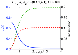
Figure 14: $g_{2}(\tau=0)$ reaches the steady-state after a time interval which is set by the bandwidth of the system, one-photon state (green) is partially transmitted while the transmission of the two-photon state (red) is further suppressed due the nonlinear dispersion. This has been generated for a system with $\Gamma_{1D}/\Gamma=10\%$ an OD=160.

First, we note that the single-photon wave function is not affected by the presence of the nonlinearity and will be perfectly transmitted in the absence of linear losses. Thus, in our truncated Hilbert space, the only subspace affected by $\kappa$ is the two-photon wave function, which is shown in Fig. 15. We clearly observe that the nonlinearity causes repulsion between two photons inside the system, as the wave function along the diagonal $z_{1}=z_{2}$ becomes suppressed while the off-diagonal amplitudes become peaked (indicating the de-localization of the photons). This behavior closely resembles that of the natural modes of the system, as calculated in Sec. VI. A similar behavior involving the “self-organization” of photons in an NLSE system in equilibrium has been discussed in Ref. Chang et al. (2008).

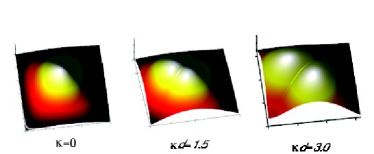
Figure 15: Two-photon wave function $|\phi(z_{1},z_{2})|$ exhibiting delocalization. We have assumed no dissipation ($\Gamma^{\prime}=\Gamma=0$) in this plot. $d=30$ for different values of $\kappa$.

In the presence of linear absorption (discussed in Sec. III), the system will not be perfectly transmitting even on resonance, and therefore in a realistic situation the transmittivity will be less than one $(T_{1}<1)$. Note, however, that such absorption would result in a classical output given a classical input. Significantly, in the presence of a nonlinearity, we find that the output light can acquire non-classical character. Specifically, the transmitted light exhibits anti-bunching ($g_{2}(z=d,\tau=0)<1$), which becomes more pronounced with increasing ${\kappa}d^{2}$ (Fig. 16). This effect partly arises from the suppression of transmission of two-photon components, due to an extra nonlinear phase shift that shifts these components out of transmission resonance. In fact, these components are more likely to get reflected, which causes the reflected field to subsequently exhibit bunching behavior. We note that this effect is similar to photon blockade in a cavity (e.g., see Refs.Imamoglu et al. (1997); Grangier et al. (1998); Imamoglu et al. (1998)). In addition, additional anti-bunching occurs due to the fact that two-photon components inside the system tend to get repelled from each other. This effect arises due to the spatial degrees of freedom present in the system, which is fundamentally different than switching schemes proposed in optical cavities (e.g., Refs.Imamoglu et al. (1997); Grangier et al. (1998); Imamoglu et al. (1998)) or wave-guides coupled to a point-like emitter Shen and Fan (2007); Chang et al. (2007). In the limit where $\kappa\rightarrow\infty$, the transmitted field approaches perfect anti-bunching, $g_{2}(d,\tau=0)=0$.

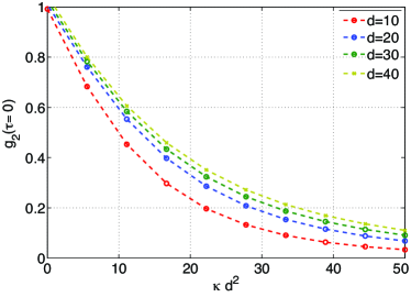
Figure 16: $g_{2}(\tau=0)$ as a function of nonlinearity. For large system sizes $d\gg 1$, the anti-bunching of the system scales with $\kappa d^{2}$.

In an experimental realization, the requirement to see the photon repulsion ($\kappa d^{2}\geq 40$) for a system with $\Gamma_{1D}/\Gamma=10\%$, would be a coherent optical length of $d\simeq 40$ when $\Delta_{2}/\Gamma=1$. Therefore, at least an optical density of $OD\simeq 160$ is needed for $T_{1}\simeq 20\%$. The anti-bunching in the transmitted light is more pronounced as the optical density increases, which increases the effective system finesse (Fig.  17).

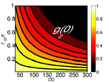
Figure 17: Repulsive photons: Correlation function $g_{2}(\tau=0)$ of the transmitted light when the frequency is set to the single-photon transmission resonance with $T_{1}\simeq 20\%$ and $\frac{\Delta_{2}}{\Gamma}=5$.

VII.2 Attractive Interaction $(\kappa<0)$

In this section, we study the quantum transport properties of the system in the presence of dispersive nonlinearity with negative coefficient. Contrary to the semi-classical prediction, we show that the second-order correlation function of the transmitted field oscillates as function of nonlinear interaction strength and can exhibit both bunching and anti-bunching. We explain the origin of this behavior in terms of the analytical solutions obtained in Sec. VI.2.

In Fig. 18(a), we plot $g_{2}(\tau=0)$ for the transmitted field versus ${\kappa}d$. Initially, the system exhibits anti-bunching behavior for small values of $|\kappa|d$  which indicates that multi-photon components tend to switch themselves out of transmission resonance. However, as we increase $|\kappa|d$, oscillations develop in the correlation function, exhibiting strong bunching behavior at particular values of ${\kappa}d$. Thus, unlike the repulsive case, a competing behavior arises between the photon switching effect and the resonant excitation of specific bound states within the system, as we describe below. In particular, the bound state energies $E_{n}^{b}$ decrease quadratically with changing $\kappa$, according to Eq. (74) or Eq. (73), which is shown in Fig. 18(b). For a fixed detuning $\delta$, the oscillation peaks (where $g_{2}$ is largest) correspond to situations where the energy of a bound state becomes equal to the energy of two incoming photons ($E_{n}^{b}=2\delta$). This effect is further confirmed by examining the two-photon wave function at each of these oscillation peaks (Fig. 18a). We clearly observe that these wave functions correspond to the bound states calculated in Sec. VI.2. Similar to Fig. 11 and Fig. 13, it is readily seen that the wave functions at these peaks are localized along the diagonal, indicating a bound state in the relative coordinates and leading to the bunching effect in transmission. On the other hand, an increasing number of nodes and anti-nodes develop along the diagonal for increasing $|\kappa|d$, which are associated with the higher momenta of the center-of-mass motion. We note that such resonances deviate significantly from the the semiclassical picture, where anti-bunching was predicted for both positive and negative nonlinearity. We also note that in cavity QED systems this effect is not present since these systems are single-mode.

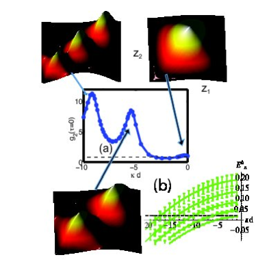
Figure 18: (a) Output correlation function $g_{2}(\tau=0)$ as a function of nonlinearity: When the negative nonlinear strength is changed to higher values and $g_{2}$ exhibits resonances at certain values of $\kappa d\simeq(0,6,10,14,...)$. In this plot the system size is $d=30$, however, for other system size same behaviors were observed around similar values of $\kappa d$. The two-photon wavefunction ($|\phi(z_{1},z_{2})|$) for four values of nonlinearity is shown. (b) Corresponding bound state energies (green-solid) which become resonant with incoming photon energy (black-dotted) for specific nonlinearities. We have assumed no dissipation ($\Gamma^{\prime}=\Gamma=0$) in these plots.

The experimental requirement to see such behaviors is more stringent than the photon repulsion in the previous section. For example, if we want to observe the second photonic bound state ($\kappa d\geq 5$) for a system with $\Gamma_{1D}/\Gamma=0.2$, the coherent optical length should be at least $d\simeq 200$ when $\Delta_{2}/\Gamma=-5$. To achieve a reasonable signal (linear transmission $T_{1}=1\%$) an optical density of $OD=3500$ is needed. Importantly, however, we have shown that the presence of bound states inside the nonlinear medium can be probed with classical light, simply by examining higher-order correlation functions in the output field, rather than sending in complicated quantum inputs.

VII.3 Dissipative Regime $(\kappa=i|\kappa|)$

In this section, we study the transport properties of the system in the presence of nonlinear absorption, and calculate its effect on the transmitted light and its correlation functions.

A purely absorptive nonlinearity arises when the detuning $\Delta_{2}$ is set to zero in our atomic system (see Fig. 1(a)). This nonlinear loss also leads to anti-bunching in the transmitted field, as multi-photon components become less likely to pass through the waveguide without being absorbed. Linear absorption, on the other hand, affects transmission of single- and multi-photon components equally. Fig. 19 and Fig. 20 show how two-photon and one-photon states are transported differently in the nonlinear absorptive system (realistic linear losses are included in this calculation).

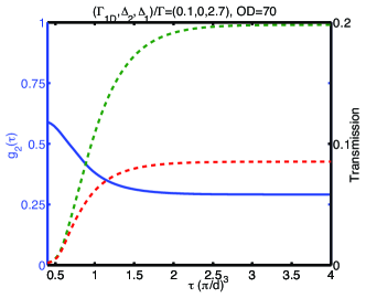
Figure 19: $g_{2}(\tau=0)$ reaches the steady-state after a time interval which is set by the bandwidth of the system, one-photon state (green) is partially transmitted while the two-photon state (red) is strongly attenuated due the nonlinear absorption. This plot has been generated for a system with $\Gamma_{1D}/\Gamma=10\%$ an OD=70.

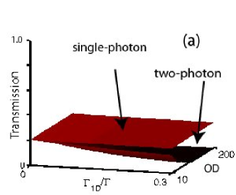
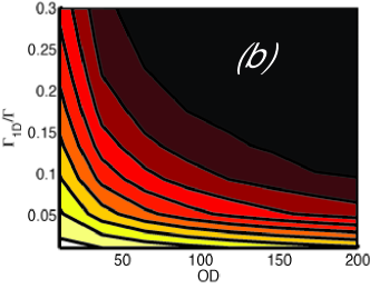
Figure 20: (a) one-photon state is partially transmitted ($T_{1}$) while the two-photon state transmission ($T_{2}$) is suppressed due the nonlinear absorption. This suppression is more pronounced for higher optical density and cooperativity. (b) Correlation function $g_{2}(\tau=0)$ of the transmitted light when the frequency is set to the single-photon transmission resonance with $T\simeq 20\%$ and $\frac{\Delta_{2}}{\Gamma}=0$.

We note that the two-photon wavefunction is attenuated due the nonlinear absorption, while it is not deformed, as shown in Fig. 21. In an experimental realization of such a system with $\Gamma_{1D}/\Gamma=10\%$, an optical coherent length of $d\simeq 20$ is enough to yield a relatively large anti-bunching ($g_{2}<0.3$). In order to have high transmission ($T_{1}=20\%$) for single photons an optical density of $OD\simeq 70$ is required.

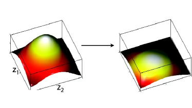
Figure 21: In the presence of the nonlinear absorption ($\frac{\Delta_{2}}{\Gamma}=0$), the two-photon wave function is strongly suppressed comparing to the absence of the nonlinear absorption ($\Delta_{2}\gg\Gamma$). These plots has been generated for a system with $\Gamma_{1D}/\Gamma=10\%$, $T_{1}\simeq 20\%$ and OD=70.

All of the physics related to the photon correlation function is described again by product of the coherent optical length and the nonlinearity coefficient $(|\kappa|d)$ (since the nonlinear absorption is equal to the nonlinear absorption coefficient times the length of the medium). However, for a fixed optical density, since the nonlinear transition is on resonance, the magnitude of the nonlinear coefficient $|\kappa|$ is enhanced compared to the nonlinear dispersive case. We note that in the presence of nonlinear absorption, one has to also consider the effect of accompanied noise. However, the effect of noise for an ensemble of many atoms which are driven by a weak laser field, is negligible, and therefore, using the NLSE with a decay term is sufficient and consistent. A rigorous demonstration of the validity of such approximation is the subject of further research.

VIII Conclusions

We have developed a technique to study few-photon quantum dynamics inside 1D nonlinear photonic system. This technique allows us to study the system even in regimes where nonlinearities are significant even at a few-photon level, where we find that the behavior of the system deviates significantly from estimates based on classical formalism. Specifically, when the system is driven by classical light, the strong optical nonlinearity manifests itself in the correlation functions of the outgoing transmitted light. In particular, when the interaction between photons is effectively repulsive, the suppression of multi-photon components results in anti-bunching of the transmitted field and the system acts as a single-photon switch. In the case of attractive interaction, the system can exhibit either anti-bunching or bunching, associated with the resonant excitation of bound states of photons by the input field. These effects can be observed by probing statistics of photons transmitted through the nonlinear fiber.

Appendix A EIT-Bandgap

In this appendix, we show that how in an EIT system, where the control field is a standing wave, a band gap structure can be developed. In particular, we show the presence of transmission resonances at the band gap edge by taking into account the full expression for the atomic susceptibilities. We show that at the band gap edge, we recover that same resonances that we presented in the main text for small detunings.

We consider a $\lambda$-level scheme, where a standing control field has coupled the forward- and backward-going probe together, similar to Fig.1 without the nonlinear transition (c-d). Following André (2005), we assume the noises to be negligible, and therefore, the atomic equations of motion to the leading order in $\mathcal{E_{\pm}}$ are

$$\partial_{t}\hat{\sigma}_{ab}^{+} = +(i\Delta_{1}-\Gamma/2)\hat{\sigma}_{ab}^{+}+i\Omega\hat{\sigma}_{ac}+ig\sqrt{2\pi}\mathcal{E}_{+}$$ (88)

$$\partial_{t}\hat{\sigma}_{ab}^{-} = +(i\Delta_{1}-\Gamma/2)\hat{\sigma}_{ab}^{-}+i\Omega\hat{\sigma}_{ac}+ig\sqrt{2\pi}\mathcal{E}_{-}$$ (89)

$$\partial_{t}\hat{\sigma}_{ac} = -\gamma_{0}\hat{\sigma}_{ac}+i\Omega\hat{\sigma}_{ab}^{+}+i\Omega\hat{\sigma}_{ab}^{-}$$ (90)

and the evolution equation of the photonic fields are written as:

$$(\partial_{t}+c\partial_{z})\mathcal{E}_{+} = i\Delta K\mathcal{E}_{+}+ig\sqrt{2\pi}n_{0}\hat{\sigma}_{ab}^{+}$$ (91)

$$(\partial_{t}-c\partial_{z})\mathcal{E}_{-} = i\Delta K\mathcal{E}_{-}+ig\sqrt{2\pi}n_{0}\hat{\sigma}_{ab}^{-}.$$ (92)

The wave-vector mismatch can be ignored by including a small shift in the two-photon detuning. By taking the Fourier transform of the atomic equation of motion, one can solve for atomic polarization and obtain the self- and cross-susceptibilities. We can define a unit length based on the absorption length $L_{abs}=\frac{c\Gamma}{2\pi g^{2}n_{0}}$, and write the field equation as:

$$\partial_{\tilde{z}}\mathcal{E}_{+} = i\tilde{\Delta}_{3}\mathcal{E}_{+}+i\chi_{s}(\delta)\mathcal{E}_{+}+i\chi_{c}(\delta)\mathcal{E}_{-}$$ (93)

$$-\partial_{\tilde{z}}\mathcal{E}_{-} = i\tilde{\Delta}_{3}\mathcal{E}_{-}+i\chi_{s}(\delta)\mathcal{E}_{-}+i\chi_{c}(\delta)\mathcal{E}_{+}$$

where the self- and cross susceptibilities and the detuning are given by:

$$\chi_{s}(\delta) = i\frac{\Gamma}{\Gamma^{\prime}}\frac{\Gamma^{\prime}\Gamma_{0}+\Omega^{2}}{\Gamma^{\prime}\Gamma_{0}+2\Omega^{2}}$$ (94)

$$\chi_{c}(\delta) = -i\frac{\Gamma}{\Gamma^{\prime}}\frac{\Omega^{2}}{\Gamma^{\prime}\Gamma_{0}+2\Omega^{2}}$$ (95)

$$\tilde{\Delta}_{3} = \frac{\Delta_{3}}{\Gamma}\frac{\Gamma^{2}}{2\pi g^{2}n_{0}}=\frac{\delta}{\eta}\frac{\Gamma}{|\Delta_{1}|}$$ (96)

where $\Gamma^{\prime}=\Gamma/2-i\Delta_{1}-i\Delta_{3}$ , $\Gamma_{0}=\gamma_{0}-i\Delta_{3}$ and $\Delta_{3}$ is the two-photon detuning of the probe from the pump field which is related to the dimensionless two-photon detuning in the main text ($\Delta_{3}=2\frac{\Omega^{2}}{\Delta_{1}}\delta\ll\Delta_{1}$). We note that in most cases, $\tilde{\Delta}_{3}$ is very small for slow group velocities ($\frac{\Gamma^{2}}{2\pi g^{2}n_{0}}=(\frac{\Gamma}{\Omega})^{2}\frac{\Omega^{2}}{2\pi g^{2}n_{0}}\ll 1$), and therefore the corresponding term can be neglected for simplicity.

In order to obtain transmission and reflection coefficient, one should solve the couple mode equations Eq.(93) with proper boundary conditions. Therefore, we consider a system which is driven with a weak coherent field at $(z=0)$. Therefore, the boundary conditions can be set to,

$$\mathcal{E}_{+}(z=0) = \mathcal{E}_{0}$$ (97)

$$\mathcal{E}_{-}(z=d) = 0.$$ (98)

We evaluate the transmission coefficient $(\mathcal{E}_{+}(z=d)/\mathcal{E}_{0})$, and the reflection coefficient $(\mathcal{E}_{-}(z=0)/\mathcal{E}_{0})$ by numerical methods using BVP5C in Matlab. In particular, we are interested in the Raman regime, in other words the detuning is very large $|\Delta_{1}|\gg\Gamma$ and also we assume $\Delta_{1}<0$. First, we consider the case where the EIT width is smaller than the one-photon detuning, i.e. $\Omega\ll|\Delta_{1}|$. Fig.22 shows the reflectivity and transmittivity of the system for different optical densities. In the regime with low optical density, the spectrum corresponds to a shifted Raman transition at $\Delta_{3}\simeq 2\frac{\Omega^{2}}{\Delta_{1}}$ and an EIT window around $\Delta_{3}\simeq-\Delta_{1}$. In higher optical densities, the system develops a band gap for $-\Omega\leq\Delta_{3}\leq 0$. Fig.22 shows that in media with higher optical density, the band gap becomes more prominent.

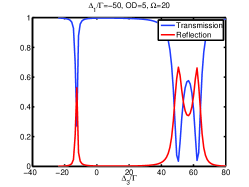
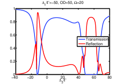
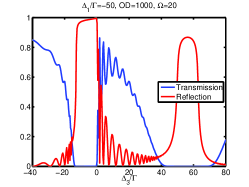
Figure 22: By increasing OD, the band gap structure becomes more pronounced

As we discussed in the main text, we are interested in the band gap edge where the transmission peaks are present and the system acts like an effective cavity. Fig.23 shows a close-up of the transmittivity and reflectivity spectrum in Fig.22(c) at the band gap edge. We can observe that several resonances occur at the edge due to the finite size of the system. By positioning at the one of the transmission peaks, the system behaves as an effective cavity, where the decay rate of the cavity will be given by the width of the transmission peak. Therefore, the present results, including the full susceptibilities of the system, is consistent with the model presented earlier where we had approximated the system to be around $\Delta_{3}=0$.

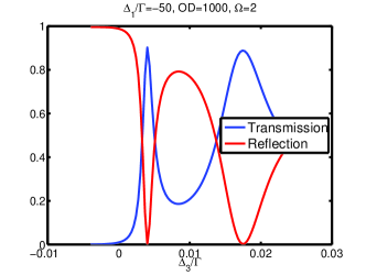
Figure 23: Transmission resonances at the edge of the band gap

We add that alternatively, one can assume a strong control field so that the EIT windows would be smaller than the one-photon detuning $\Omega>|\Delta_{1}|$. Similar to the previous case $\Omega<|\Delta_{1}|$, the system develops a band gap. As shown in Fig.24, the band gap is formed between $-\Omega\lesssim\Delta_{3}\lesssim\Omega$, similar to modulated EIT with AC-stark shift as discussed in Ref.André and Lukin (2002).

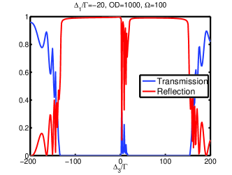
Figure 24: Band gap structure for strong control fields $(\Omega>\Delta_{1}$)

Appendix B Numerical Methods

In this section, we describe the numerical methods that have been used to simulate the evolution of the photonic quantum state and the related correlation functions, in the limit where we truncate the Hilbert space to two photons or less. The partial differential equations for the one-photon and two-photon wave functions (27, 28) are turned into difference equations by discretizing space and time, and are evolved forward in time using the Du Fort-Frankel scheme Strikwerda (2004). This algorithm is is explicit in time – i.e., the next time step function is explicitly given by the past time function – and is also unconditionally stable. We note that the system under investigation is open and it is driven out of equilibrium, therefore, conventional analytical methods for approaching the NLSE such as Bethe ansatz or quantum inverse scattering Korepin et al. (1993) are not applicable here.

The one-photon wave function can be easily integrated and solved analytically. However, we describe how to obtain the one-photon wave function numerically and then generalize this technique to obtain the two-photon wave function. First, we mesh space and time and reduce the differential equations to a difference equation. If we choose the time step $k$ and the space step $h$, the discretized time and space will be $x=z/h$ and $s=t/k$ and the system length $d=Nh$. Then following the Du Fort-Frankel scheme Strikwerda (2004), the evolution equation takes the form:

$$\frac{\theta(x,s+1)-\theta(x,s-1)}{2k} = \frac{i}{2mh^{2}}[\theta(x+1,s)+\theta(x-1,s)$$ (99)

$$- \theta(x,s+1)-\theta(x,s-1)]$$

where the position take all values inside the boundary ($2\leq x\leq N-1$). By rearranging the above equation, the explicit form of the equation can be obtained

$$( 1 +~{}\frac{ik}{mh^{2}})\theta(x,s+1)=\theta(x,s-1)$$

$$+ \frac{ik}{mh^{2}}\left[\theta(x+1,t)+\theta(x-1,t)-\theta(x,s-1)\right]$$

Therefore inside the boundaries, the wave function at time $s+1$ can be obtained knowing the wave function at time $s$ and $s-1$. The boundary condition at $z=0$ -i.e. $x=1$, will be given by

$$\alpha = \frac{\theta(1,s+1)+\theta(2,s+1)}{2}$$

$$- i\frac{\theta(2,t+1)-\theta(1,s+1)}{2mh}$$

Or equivalently,

$$\theta(1,s+1)=\frac{\alpha+(-\frac{1}{2}+\frac{i}{2mh})\theta(2,s+1)}{\frac{1}{2}+\frac{i}{2mh}}$$ (102)

and similarly for the boundary condition at $z=d$ -i.e. $x=N$, we have

$$\theta(N,s+1)=\frac{(-\frac{1}{2}+\frac{i}{2mh})\theta(N-1,s+1)}{\frac{1}{2}+\frac{i}{2mh}}.$$ (103)

Therefore, by having the above boundary conditions and the initial condition $\theta(x,s=1)=0$, the wave function can be calculated at any time inside the boundaries ($2\leq x\leq N-1$). The order of accuracy of the Du Fort-Frankel scheme is given by $O(h^{2})+O(k^{2})+O(k^{2}h^{-2})$ and it is consistent as $k/h$ tends to zero Strikwerda (2004).

Similarly, we can write a difference equation for the two-photon wave function. The $\delta$-interaction can be approximated by a Gaussian distribution. The space domain is meshed so that $\Delta z_{1}=\Delta z_{2}=h$. The evolution equation for the two-photon wave function reads

$$\left(1+\frac{2ik}{mh^{2}}\right)\phi(x,y,s+1)=$$

$$\frac{ik}{mh^{2}}\left[\phi(x+1,y,s)+\phi(x-1,y,s)\right]$$

$$+\frac{ik}{mh^{2}}\left[\phi(x,y+1,s)+\phi(x,y-1,s)\right]$$

$$+2\frac{ik}{mh^{2}}\phi(x,y,s-1)+\phi(x,y,s-1)$$

$$-2k\frac{2i\kappa}{\sigma\sqrt{2\pi}}{\rm{Exp}\left(-\frac{(x-y)^{2}}{2\sigma^{2}}\right)\phi(x,y,s)}$$

The boundary condition at $z=0$ will be given by

$$\frac{\alpha}{2}\theta(y,s+1) = \frac{\phi(1,y,s+1)+\phi(2,y,s+1)}{2}$$

$$- i\frac{\phi(2,y,s+1)-\phi(1,y,s+1)}{2mh},$$

where $\sigma$ is the length scale characterizing the distance of the two-photon interaction. Approximating the delta-function with a Gaussian is valid if $\sigma\ll d$. On the other hand, we should have $h\ll\sigma$ so that the Gaussian function would be smooth. Or equivalently,

$$\phi(1,y,s+1)=\frac{\frac{1}{2}\alpha\theta(y,s+1)+(-\frac{1}{2}+\frac{i}{2mh})\phi(2,y,s+1)}{\frac{1}{2}+\frac{i}{2mh}}$$ (106)

and similarly for the boundary condition at $z=d$, we have

$$0 = \frac{\phi(N,y,s+1)+\phi(N-1,y,s+1)}{2}$$

$$+ i\frac{\phi(N,y,s+1)-\phi(N-1,y,s+1)}{2mh}$$

which gives

$$\phi(N,y,s+1)=\frac{(-\frac{1}{2}+\frac{i}{2mh})\phi(N-1,y,s+1)}{\frac{1}{2}+\frac{i}{2mh}}.$$ (108)

Once the wave function is known at any point in time and space, we can evaluate the correlation functions. In particular, the two-photon correlation function $g_{2}(d,\tau=0)$ is given by Eq. (40), where the first and the second derivatives at anytime are given by the following expressions,

$$\partial^{(1)}\phi(d,d) = \frac{1}{2mh}[\phi(N,N)-\phi(N-1,N)]$$ (109)

$$\partial^{(1)}\partial^{(2)}\phi(d,d) = \frac{1}{4m^{2}h^{2}}[\phi(N,N)-\phi(N-1,N)$$

$$- \phi(N,N-1)+\phi(N-1,N-1)].$$

Note that in evaluation of $g_{2}(\tau)$, once the first photon is detected the two-photon wave function collapses to zero. This seems to be contradictory with the driven boundary condition Eq.(33) where the two-photon state at the boundaries is proportional to the one-photon wave function which is not zero. This apparent inconsistency occurs because we have neglected higher number photon states in our truncation. However, this inconsistency only leads to higher order corrections to $g_{2}(\tau)$ in the input field amplitude $\alpha$, which is assumed to be weak ($\alpha{\ll}1$).