Correlated two–photon emission by transitions of Dirac–Volkov states in intense laser fields: QED predictions

Abstract

In an intense laser field, an electron may decay by emitting a pair of photons. The two photons emitted during the process, which can be interpreted as a laser-dressed double Compton scattering, remain entangled in a quantifiable way: namely, the so-called concurrence of the photon polarizations gives a gauge-invariant measure of the correlation of the hard gamma rays. We calculate the differential rate and concurrence for a backscattering setup of the electron and photon beam, employing Volkov states and propagators for the electron lines, thus accounting nonperturbatively for the electron-laser interaction. The nonperturbative results are shown to differ significantly compared to those obtained from the usual double Compton scattering.

I Introduction

In perturbative double Compton scattering Eliezer (1946); Mandl and Skyrme (1952); Bell (2008), an incoming photon interacts with an electron, and two photons are emitted. This process, which is represented by the Feynman diagrams in Fig. 1, can be described by perturbative quantum electrodynamics (QED) and requires no other special theoretical input. Experimental evidence ranges from the first measurements more than 50 years ago Cavanagh (1952); Theus and Beach (1957); McGie et al. (1966) to the more recent Sekhon et al. (1988); Sandhu et al. (1999); Saddi et al. (2006, 2008). However, if the emission process takes place inside an intense laser field, then the physics changes, and the electron line is dressed by multiple interactions with the laser field (see Fig. 2). The emission of two photons is a purely quantum process which cannot be described by classical radiation theory Melrose (1972). An exception is encountered only for the case of the sequential emission of two quanta which occurs when the intermediate propagator hits a resonance pole, given by a resonant Dirac–Volkov state. In that case, to which we will return to later in the paper, the diagrams in Fig. 2 break apart into two distinctive blocks for the emission of the two photons.

Figure 1: The 6 Feynman diagrams contributing to (ordinary) double Compton scattering (initial electron four momentum $p_{i}$, final four momentum $p_{f}$). The electron line is denoted by a single customary fermion line. The frequencies of the two emitted photons with wave four vectors $k_{b}$ and $k_{c}$ may be different and thus may be their wavelengths; this is explicitly indicated in the panel.

The most interesting geometry for the process is the backscattering case, where a relativistic electron counterpropagates against an intense laser beam of comparatively low frequency (on the order of a few eV). In ordinary Compton scattering, the electron is usually assumed to be at rest, and the scattering of a highly energetic photon is considered. Because the kinematics is inverted in the backscattering case, one sometimes refers to this scenario as “inverse Compton scattering”. During the emission, the electron interacts with the laser field via an arbitrary number of interactions (see Fig. 2); the process can be described by fully laser-dressed Dirac–Volkov propagators Reiss and Eberly (1966); Lötstedt et al. (2007). So, we may refer to the process depicted in Fig. 2 as “inverse laser-dressed double Compton backscattering.”

Figure 2: Feynman diagram for the two-photon decay of a Dirac–Volkov state. The electron line is dressed by the laser field and denoted by a zigzag laser photon superimposed on the fermion line.

Note that for a single-photon Compton backscattering, the highest photon energy attainable is $4\gamma^{2}\omega$, where $\omega$ is the laser photon energy and $\gamma$ is the Lorentz factor of the incoming electron. For a defined scattering geometry, the energy of the emitted photon thus is uniquely defined, and it coincides with the energy of the emitted classical (Larmor) radiation in the specified direction provided the laser photon energy is much smaller than the electron mass and Lorentz boost factors are taken into account. If the electron absorbs $n$ laser photons during laser-dressed single Compton scattering, the energy maximum changes to $4n\gamma^{2}\omega/(1+\xi^{2})$, where the laser intensity parameter $\xi$ is defined in Eq. (6) below ($\xi^{2}$ is proportional to the laser intensity). When two photons are emitted in laser-dressed double Compton scattering, their maximum energy sum is limited by $\omega_{1}+\omega_{2}\leq 4n\gamma^{2}\omega/(1+\xi^{2})$. As we will show, it is possible to designate energy and angular regions in which the double scattering process dominates over single scattering, which is crucial for an experimental verification Brodin et al. (2008); Thirolf et al. (2009).

Interestingly, as noted in Schützhold et al. (2006, 2008); Schützhold and Maia (2009), the two photons emitted during the process are entangled because of the quantum nature of the process. In order to quantify the entanglement, the emission directions of the two quanta cannot be used with good effect, because they represent continuous variables in three dimensions. However, the polarization components of the two photons along the emission lines can be uniquely decomposed in a two-dimensional space composed of unit vectors (effectively a one-dimensional space), and measured independently. Triggering on simultaneous two-photon events, one can then measure the entanglement quantitatively: an appropriate measure is the so-called concurrence Wootters (1998); Cirone (2005) which measures the polarization entanglement of the two quanta.

The usual double Compton scattering, which involves the absorption of only one laser photon, has a rate which is proportional to the square of the laser four-vector amplitude, i.e., proportional to its intensity. Therefore, we may refer to the single scattering process as the “linear” process. With rising laser intensity, the rate deviates from the simple linear intensity dependence, it becomes more and more indispensable to include higher-order effects, and the process becomes nonlinear.

In order to bring the current investigation into perspective, we would like to mention other work performed in connection with two-photon emission from free electrons: indeed, a pair of photons may be produced by electrons accelerated by any kind of external field. Probably the most well known process of this kind is double bremsstrahlung Baier et al. (1981); Altman and Quarles (1985); Véniard et al. (1987); Hippler (1991); Kahler et al. (1992); Korol (1997); Dondera and Florescu (1998); Krylovetskiĭ et al. (2002); Korol and Solovjev (2006), but also photon pair creation in a magnetic field Zhukovskiĭ and Nikitina (1973); Sokolov et al. (1976); Fomin and Kholodov (2003), and in a crossed field Morozov and Ritus (1975) has been considered. The process under investigation in this paper is complementary to those mentioned above, and may provide for better control of the properties of the produced photons by adjusting the laser parameters.

This paper is organized as follows. In Sec. II, we discuss the formulation in terms of a laser-dressed (“nonperturbative”) QED formalism. We then continue, in Sec. III, with a comparison of the predictions of the fully relativistic, nonperturbative theory to the relativistic, but perturbative (in the laser field) theory of double Compton scattering. In particular, we extend the discussion given in Ref. Lötstedt and Jentschura (2009a) to also include circularly polarized laser fields. In Sec. IV, we study the angular correlation and the entanglement of the emitted photons, in the nonperturbative formalism. Finally, conclusions are drawn in Sec. V. Throughout the paper, we use relativistic natural units such that $\hbar=c=1$, and a space-time metric $g^{\mu\nu}={\rm diag}(1,-1,-1,-1)$. Scalar products of four-vectors are written as $p_{\mu}q^{\mu}=p\cdot q$ for two four-vectors $p$ and $q$. The gamma matrices are written as $\gamma^{\mu}$, and their contraction with a four-vector $p$ as $\hat{p}=\gamma\cdot p$.

II Formulation of the QED theory

II.1 Notation

The electron mass is denoted by $m$, and the electron charge by $e=-|e|$. The laser wave vector points in the negative $x^{3}$ direction [with the space-time coordinate $x^{\mu}=(x^{0},\bm{x})=(x^{0},x^{1},x^{2},x^{3})$],

$$\varkappa^{\mu}=(\omega,\bm{\varkappa})=\omega\,(1,0,0,-1),$$ (1)

and the laser four-vector potential, modeled as a monochromatic plane wave, for linear polarization is

$$A_{\text{lin}}^{\mu}(\phi)=a^{\mu}\cos\phi,\qquad\phi=\varkappa\cdot x,$$ (2)

with $a\cdot\varkappa=0$, $a^{\mu}=|a|(0,1,0,0)$. For circular polarization we have instead,

$$A_{\text{circ}}^{\mu}(\phi)=a_{1}^{\mu}\cos\phi+a_{2}^{\mu}\sin\phi,$$ (3)

with $a_{1}\cdot a_{2}=0$, $a_{2}^{2}=a_{1}^{2}$, $a_{1}^{\mu}=|a_{1}|(0,1,0,0)$, $a_{2}^{\mu}=|a_{1}|(0,0,1,0)$. The laser intensity parameter $\xi$ is defined as

$$\xi=\frac{-e}{m}\sqrt{\frac{-a^{2}}{2}},$$ (4)

for linear, and

$$\xi=\frac{-e\sqrt{-a_{1}^{2}}}{m}=\frac{-e}{m}\sqrt{\frac{-a_{1}^{2}-a_{2}^{2}}{2}}.$$ (5)

for circular polarization. For a consistent comparison of linear and circular polarization, one should compare at the same value of $\xi$, which corresponds to the same laser intensity. The parameter $\xi$ relates to the root-mean-square electric field amplitude $\bar{E}$ like

$$\xi=\frac{-e\bar{E}}{m\omega},$$ (6)

and can be said to be the relativistic (inverse of the) Keldysh parameter: $\xi<1$ corresponds to the multiphoton regime of relativistic laser-matter interaction, where the coupling to the laser field is perturbative, and $\xi>1$ is commonly referred to as the tunneling, or nonperturbative regime. The quantum parameter $\chi$ Ritus (1979), which in general determines the magnitude of quantum effects such as $e^{+}e^{-}$ pair creation, spin effects etc, is defined as

$$\chi=\xi\,\frac{p_{i}\cdot\varkappa}{m^{2}},$$ (7)

where $p_{i}$ is the initial momentum of the electron [see Eq. (II.1)]. If we compute $\chi$ in the rest frame of the electron, where $p_{i}=(m,\bm{0})$, then

$$\chi=\xi\frac{\omega}{m}=\frac{\bar{E}}{E_{\textrm{crit}}},$$ (8)

where $E_{\textrm{crit}}=m^{2}/|e|$ is the critical (Schwinger) field. Thus, $\chi$ is the amplitude of the electrical field of the laser compared to the critical field in the rest frame of the electron. The relation to laser intensities follows from the formula

$$I=\xi^{2}\left(\frac{\omega}{m}\right)^{2}I_{\textrm{crit}},$$ (9)

where $I_{\textrm{crit}}=2.3\times 10^{29}$ W/cm² is the critical intensity, corresponding to $\chi=1$ in the lab frame. For most of our examples, we use $\omega=2.5$ eV (optical laser), which corresponds to $I=5.5\times 10^{18}$ W/cm² for $\xi=1$ and $I=2.2\times 10^{19}$ W/cm² for $\xi=2$; the laser field here is strong but manifestly sub-critical. Note that even in the case of a relativistic (Lorentz factor $\gamma=10^{3}$) electron beam as considered later in the examples (see Secs. II.5 and III), the laser field remains sub-critical in the rest frame of the electron, since $\chi=\xi p_{i}\cdot\varkappa/m^{2}\approx 10^{-2}\ll 1$ with the parameters chosen.

The initial electron four-momentum is (we assume the electron to be counterpropagating with respect to the laser field, i.e., moving in the positive $x^{3}$-direction):

$$p_{i}= \;(E_{i},\bm{p}_{i})=(E_{i},0,0,\sqrt{E_{i}^{2}-m^{2}}),$$

$$q_{i}= \;p_{i}+\xi^{2}\frac{m^{2}}{2\varkappa\cdot p_{i}}\,\varkappa=(Q_{i},\bm{q}_{i})\,,$$ (10)

which is valid for both circular and linear polarization. The final electron four-momentum is

$$p_{f}=\;(E_{f},\bm{p}_{f}),\quad q_{f}=p_{f}+\xi^{2}\frac{m^{2}}{2\varkappa\cdot p_{f}}\,\varkappa=(Q_{f},\bm{q}_{f}).$$ (11)

The four-vector $q_{i,f}$ introduced in Eqs. (II.1), (11) is the average momentum of a laser-dressed electron Ritus (1979), with corresponding average mass $m_{\ast}$,

$$q_{f}^{2}=\;q_{i}^{2}=m_{\ast}^{2}=m^{2}(1+\xi^{2}).$$ (12)

The electron spinors are used in the following form:

$$u_{r}(p)=\sqrt{\frac{E+m}{2m}}\left(\begin{array}[]{c}\delta_{r1}\\ \delta_{r2}\\ \frac{1}{E+m}\bm{\sigma}\cdot\bm{p}\binom{\delta_{r1}}{\delta_{r2}}\end{array}\right),$$ (13)

with the standard vector $\bm{\sigma}$ being composed of the (Pauli) $2\times 2$ spin matrices. With this convention, the spinors are normalized according to $u_{r}^{\dagger}(p)\gamma^{0}u_{r}(p)=\bar{u}_{r}u_{r}=1$. For an electron moving in the $x^{3}$-direction, $r=1$ corresponds to a right-handed electron, and $r=2$ to a left-handed electron.

The Volkov states Ritus (1979), solutions of the Dirac equation with an external laser field

$$\left(i\hat{\partial}-m-e\hat{A}\right)\Psi=0,$$ (14)

read for linear polarization [see Eq. (2)]

$$\Psi_{p,r}(x)= \;\sqrt{\frac{m}{QV}}\,\sum_{s=-\infty}^{\infty}\left[A_{0}(s,\alpha,\beta)+\frac{e\hat{\varkappa}\hat{a}}{2\varkappa\cdot p}A_{1}(s,\alpha,\beta)\right]$$

$$\times u_{r}(p){\rm e}^{-i(q+s\varkappa)\cdot x},$$ (15)

where

$$\alpha=\frac{e\,a\cdot p}{\varkappa\cdot p},\qquad\beta=\frac{e^{2}\,a^{2}}{8\varkappa\cdot p}.$$ (16)

Here, the generalized Bessel function Reiss (1962); Korsch et al. (2006) is defined as

$$A_{k}(n,\alpha,\beta)=\;\frac{1}{2\pi}\int_{0}^{2\pi}\cos^{k}\theta\,{\rm e}^{in\theta-i\alpha\sin\theta+i\beta\sin 2\theta}\,d\theta,$$ (17)

with $k\geq 0$, from which follows $A_{k>0}(n,\alpha,\beta)=\;\tfrac{1}{2}\left[A_{k-1}(n+1,\alpha,\beta)+A_{k-1}(n-1,\alpha,\beta)\right]$.

For circular polarization [see Eq. (3)] we have,

$$\Psi_{p,r}(x)= \;\sqrt{\frac{m}{QV}}\sum_{s=-\infty}^{\infty}\left[J_{s}(\bar{\alpha})\,{\rm e}^{is\varphi}+\frac{e\,\hat{\varkappa}\,\hat{a}_{1}}{2\varkappa\cdot p}J_{s}^{+}(\bar{\alpha},\varphi)\right.$$

$$\;\left.+\frac{e\,\hat{\varkappa}\,\hat{a}_{2}}{2\varkappa\cdot p}J_{s}^{-}(\bar{\alpha},\varphi)\right]u_{r}(p){\rm e}^{-i(q-s\varkappa)\cdot x}.$$ (18)

Here

$$\bar{\alpha}=\sqrt{\alpha_{1}^{2}+\alpha_{2}^{2}},\quad\alpha_{1}=\frac{ea_{1}\cdot p}{\varkappa\cdot p},\quad\alpha_{2}=\frac{ea_{2}\cdot p}{\varkappa\cdot p},$$ (19)

and

$$\varphi=\text{arctan}_{2}\;(\alpha_{2},-\alpha_{1})\,.$$ (20)

The $\text{arctan}_{2}\;(\cdot,\cdot)$ functions is defined as

$$\text{arctan}_{2}\;(y,x) =\arctan\left(\frac{y}{x}\right)\quad\text{if }x>0,$$

$$\text{arctan}_{2}\;(y,x) =\pi+\arctan\left(\frac{y}{x}\right)\quad\text{if }x<0,$$ (21)

the usual Bessel functions are denoted by $J_{n}(\alpha)$, and

$$\begin{split}J_{s}^{+}(\alpha,\varphi)&=\frac{1}{2}\left[J_{s-1}(\alpha){\rm e}^{i(s-1)\varphi}+J_{s+1}(\alpha){\rm e}^{i(s+1)\varphi}\right],\\ J_{s}^{-}(\alpha,\varphi)&=\frac{1}{2i}\left[J_{s-1}(\alpha){\rm e}^{i(s-1)\varphi}-J_{s+1}(\alpha){\rm e}^{i(s+1)\varphi}\right]\,.\end{split}$$ (22)

Note the normalization factor in Eqs. (II.1) and (II.1): the volume $V$ comes with the wave function, and not with the spinor $u(p)$.

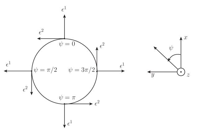
Figure 3: Polarization vectors according to Eq. (II.1) for fixed, small $\theta\approx 0$, i.e., for a photon propagating in the positive $z$ direction. For example, we have at $\psi=\pi/2$ the two vectors $\epsilon^{1}=(0,0,\cos\theta,-\sin\theta)\approx(0,0,1,0)$ and $\epsilon^{2}=(0,-1,0,0)$.

The propagation four-vectors of the two emitted photons are denoted by

$$k_{b}= \;(\omega_{b},\bm{k}_{b})=\omega_{b}\,\tilde{k}_{b}$$

$$= \;\omega_{b}\,(1,\,\sin\theta_{b}\cos\psi_{b},\,\sin\theta_{b}\sin\psi_{b},\cos\theta_{b}),$$ (23a)

$$k_{c}= \;(\omega_{c},\bm{k}_{c})=\omega_{c}\,\tilde{k}_{c}$$

$$= \;\omega_{c}(1,\,\sin\theta_{c}\cos\psi_{c},\,\sin\theta_{c}\sin\psi_{c},\cos\theta_{c}),$$ (23b)

$\psi$ measuring the azimuth and $\theta$ measuring the polar angle. As a basis for the two polarization four-vectors $\epsilon_{b}$ and $\epsilon_{c}$ of the two emitted photons, we take

$$\epsilon_{b}^{1}= \;\left(0,\,\cos\theta_{b}\,\cos\psi_{b},\,\cos\theta_{b}\,\sin\psi_{b},\,-\sin\theta_{b}\right),$$

$$\epsilon_{b}^{2}= \;\left(0,\,-\sin\psi_{b},\,\cos\psi_{b},\,0\right)$$

$$\epsilon_{c}^{1}= \;\left(0,\,\cos\theta_{c}\,\cos\psi_{c},\,\cos\theta_{c}\sin\psi_{c},\,-\sin\theta_{c}\right)\,,$$

$$\epsilon_{c}^{2}= \;\left(0,\,-\sin\psi_{c},\,\cos\psi_{c},\,0\right)\,.$$ (24)

As an aid to the discussion, Fig. 3 illustrates the direction of the polarization vectors for small polar angle $\theta$ and different values of $\psi$. Alternatively, the polarization can be expressed in a helicity basis according to

$$\begin{split}&\epsilon^{R}_{b}=\frac{1}{\sqrt{2}}(\epsilon_{b}^{1}+i\,\epsilon_{b}^{2}),\qquad\epsilon^{L}_{b}=\frac{1}{\sqrt{2}}(\epsilon_{b}^{1}-i\,\epsilon_{b}^{2}),\\ &\epsilon^{R}_{c}=\frac{1}{\sqrt{2}}(\epsilon_{c}^{1}+i\,\epsilon_{c}^{2}),\qquad\epsilon^{L}_{c}=\frac{1}{\sqrt{2}}(\epsilon_{c}^{1}-i\,\epsilon_{c}^{2}).\end{split}$$ (25)

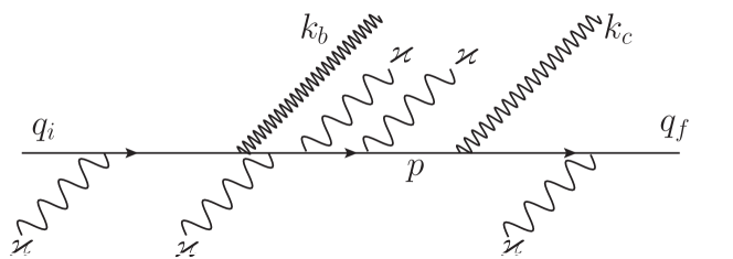
Figure 4: Clarification of the index $s$. Shown above is one of the contributing Feynman diagrams in the perturbative picture, where the laser photons are inserted one by one. The net number of laser mode absorbed photons in this case is $n=1$. The propagator momentum is $p=q_{i}-k_{b}+s\varkappa$, so that $s$ counts the net number of absorbed photons before emitting photon $k_{c}$, i.e. the momentum at the position of the label “$p$”. For the above diagram, $s=0$. Although $n$ must be positive for a net two-photon emission process, $s$ may be negative, and to get the total amplitude for fixed $n$, one should sum all diagrams of this kind with $s$ ranging from $-\infty$ to $+\infty$.

II.2 Matrix element for linear laser polarization

The $S$-matrix element for two-photon emission from a Dirac–Volkov state follows from standard Feynman rules, with four-vector potentials $\hat{A}_{b}=A^{\mu}_{b}\gamma_{\mu}=\hat{\epsilon}_{b}{\rm e}^{ik_{b}\cdot x}/\sqrt{V\,2\omega_{b}}$ and $\hat{A}_{c}=A^{\mu}_{c}\gamma_{\mu}=\hat{\epsilon}_{c}{\rm e}^{ik_{c}\cdot x}/\sqrt{V\,2\omega_{c}}$ for the two emitted photons (see also the Feynman diagram in Fig. 2). For linear laser polarization, we get

$$S_{fi}^{\text{linear}}=S_{fi}^{(1)}+S_{fi}^{(2)}$$ (26)

$$=e^{2}\int d^{4}x_{1}\!\!\int d^{4}x_{2}\overline{\psi}_{q_{f},r_{f}}(x_{2})\Big{[}i\hat{A}_{c}(x_{2})iG(x_{2},x_{1})i\hat{A}_{b}(x_{1})$$

$$\quad+i\hat{A}_{b}(x_{2})iG(x_{2},x_{1})i\hat{A}_{c}(x_{1})\Big{]}\,\psi_{q_{i},r_{i}}(x_{1})$$

$$=-i\sum_{\begin{subarray}{c}n=1\\ s=-\infty\end{subarray}}^{\infty}\frac{(2\pi)^{4}e^{2}m}{2V^{2}\,\sqrt{\omega_{c}\omega_{b}Q_{i}Q_{f}}}\,\delta^{4}(q_{i}-q_{f}+n\varkappa-k_{b}-k_{c})$$

$$\qquad\times\bar{u}_{r_{f}}(p_{f})\,\left[M_{b}^{s-n}\frac{\hat{{p}}_{b}-\xi^{2}\frac{m^{2}}{2\varkappa\cdot{p}_{b}}\hat{\varkappa}+m}{{p}_{b}^{2}-m_{\ast}^{2}}F_{b}^{s}\right.$$

$$\qquad\qquad\left.+{M}^{s-n}_{c}\frac{\hat{{p}}_{c}-\xi^{2}\frac{m^{2}}{2\varkappa\cdot{p}_{c}}\hat{\varkappa}+m}{{p}^{2}_{c}-m_{\ast}^{2}}{F}_{c}^{s}\right]u_{r_{i}}(p_{i}).$$

Here, $G(x,y)$ denotes the laser-dressed propagator function Reiss and Eberly (1966); Ritus (1979), which can be constructed from the Volkov state (II.1). The propagator momenta are given as

$${p}_{b}=\;q_{i}+s\varkappa-k_{b},\qquad{p}_{c}=q_{i}+s\varkappa-k_{c}.$$ (27)

The matrix element is proportional to $V^{-2}$, since there are one in-state and three out-states, each with a factor $\sqrt{V}$. Here, $n$ is the net number of absorbed laser photons, and the summation index $s$ can be understood as the number of laser photons absorbed up to and immediately before emitting the second photon (see Fig. 4 for a pictorial explanation).

The matrix-valued functions for the transition currents $M$ and $F$ are given as follows. For the first channel, we have

$$M_{b}^{s-n}=A_{0}(s-n,\alpha_{f}-{\alpha}_{b},\beta_{f}-{\beta}_{b})\,\hat{\epsilon}_{c}$$

$$\;+A_{1}(s-n,\alpha_{f}-{\alpha}_{b},\beta_{f}-{\beta}_{b})\,\left(\hat{\epsilon}_{c}\frac{e\hat{\varkappa}\hat{a}}{2\varkappa\cdot{p}_{b}}+\frac{e\hat{a}\hat{\varkappa}}{2\varkappa\cdot p_{f}}\hat{\epsilon}_{c}\right)$$

$$\;-A_{2}(s-n,\alpha_{f}-{\alpha}_{b},\beta_{f}-{\beta}_{b})\frac{e^{2}a^{2}\varkappa\cdot\epsilon_{c}}{2\varkappa\cdot p_{f}\varkappa\cdot{p}_{b}}\hat{\varkappa}\,,$$ (28)

and

$$F_{b}^{s}=\;A_{0}(s,\alpha_{i}-{\alpha}_{b},\beta_{i}-{\beta}_{b})\,\hat{\epsilon}_{b}$$

$$\;+A_{1}(s,\alpha_{i}-{\alpha}_{b},\beta_{i}-{\beta}_{b})\,\left(\hat{\epsilon}_{b}\frac{e\hat{\varkappa}\hat{a}}{2\varkappa\cdot p_{i}}+\frac{e\hat{a}\hat{\varkappa}}{2\varkappa\cdot{p}_{b}}\hat{\epsilon}_{b}\right)$$

$$\;-A_{2}(s,\alpha_{i}-{\alpha}_{b},\beta_{i}-{\beta}_{b})\,\frac{e^{2}a^{2}\varkappa\cdot\epsilon_{b}}{2\varkappa\cdot{p}_{b}\varkappa\cdot p_{i}}\hat{\varkappa}\,.$$ (29)

For the second channel, the two currents are given as $M_{c}^{s-n}=\;M_{b}^{s-n}(c\leftrightarrow b)$ and $F_{c}^{s}=F_{b}^{s}(c\leftrightarrow b)$ under replacements of the corresponding expressions for the first channel. The arguments entering the generalized Bessel functions read

$$\alpha_{j}=\;\frac{e\,a\cdot p_{j}}{\varkappa\cdot p_{j}},\qquad\beta_{j}=\frac{e^{2}\,a^{2}}{8p_{j}\cdot\varkappa},$$ (30)

with $j\in\{i,f,b,c\}$. The spinors $u_{r_{i,f}}$ describe the spin state of the in- and outgoing electron, respectively. Note that $\varkappa\cdot p_{i,f}=\varkappa\cdot q_{i,f}$, and that due to $\varkappa^{2}=0$, ${\alpha}_{c,b}$ and ${\beta}_{c,b}$ are independent of the summation index $s$, although one might have initially assumed a dependence on $s$ in view of the presence of $p_{b}$ and $p_{c}$ in their respective defining equations.

II.3 Matrix element for circular laser polarization

For the case of circular polarization of the laser, the matrix element can be derived in a similar way to Eq. (26). The matrix element reads

$$S_{fi}^{\text{circular}}=S_{fi}^{(1)c}+S_{fi}^{(2)c}$$ (31)

$$=-i\sum_{\begin{subarray}{c}n=1\\ s=-\infty\end{subarray}}^{\infty}\frac{(2\pi)^{4}e^{2}m}{2V^{2}\sqrt{\omega_{c}\omega_{b}Q_{i}Q_{f}}}\,\delta^{4}(q_{i}-q_{f}+n\varkappa-k_{b}-k_{c})$$

$$\times\bar{u}_{r_{f}}(p_{f})\left[N_{b}^{s-n}\frac{\hat{{p}}_{b}-\xi^{2}\frac{m^{2}}{2\varkappa\cdot{p}_{b}}\hat{\varkappa}+m}{{p}_{b}^{2}-m_{\ast}^{2}}G_{b}^{s}\right.$$

$$\;\qquad\left.+{N}^{s-n}_{c}\frac{\hat{{p}}_{c}-\xi^{2}\frac{m^{2}}{2\varkappa\cdot{p}_{c}}\hat{\varkappa}+m}{{p}^{2}_{c}-m_{\ast}^{2}}{G}_{c}^{s}\right]u_{r_{i}}(p_{i})\,.$$

Here, as is typical for circular polarization, the generalized Bessel functions in the formulas simplify to ordinary Bessel functions. The matrix-valued functions for the first channel read

$$N_{b}^{s-n}=\;J_{s-n}(\bar{\alpha}_{fb}){\rm e}^{i\varphi_{fb}(s-n)}\left(\hat{\epsilon}_{c}-\frac{e^{2}a_{1}^{2}\,\varkappa\cdot\epsilon_{c}}{2\varkappa\cdot p_{f}\varkappa\cdot{p}_{b}}\hat{\varkappa}\right)$$ (32)

$$+\Big{[}J_{s-n-1}(\bar{\alpha}_{fb}){\rm e}^{i\varphi_{fb}(s-n-1)}+J_{s-n+1}(\bar{\alpha}_{fb}){\rm e}^{i\varphi_{fb}(s-n+1)}\Big{]}$$

$$\qquad\times\frac{1}{2}\left(\hat{\epsilon}_{c}\frac{e\hat{\varkappa}\hat{a}_{1}}{2\varkappa\cdot{p}_{b}}+\frac{e\hat{a}_{1}\hat{\varkappa}}{2\varkappa\cdot p_{f}}\hat{\epsilon}_{c}\right)$$

$$+\left[J_{s-n-1}(\bar{\alpha}_{fb}){\rm e}^{i\varphi_{fb}(s-n-1)}-J_{s-n+1}(\bar{\alpha}_{fb}){\rm e}^{i\varphi_{fb}(s-n+1)}\right]$$

$$\qquad\times\frac{1}{2i}\left(\hat{\epsilon}_{c}\frac{e\hat{\varkappa}\hat{a}_{2}}{2\varkappa\cdot{p}_{b}}+\frac{e\hat{a}_{2}\hat{\varkappa}}{2\varkappa\cdot p_{f}}\hat{\epsilon}_{c}\right),$$

and

$$G_{b}^{s}=\;J_{-s}(\bar{\alpha}_{ib}){\rm e}^{-i\varphi_{ib}s}\left(\hat{\epsilon}_{b}-\frac{e^{2}a_{1}^{2}\,\varkappa\cdot\epsilon_{b}}{2\varkappa\cdot p_{i}\varkappa\cdot{p}_{b}}\hat{\varkappa}\right)$$ (33)

$$+\left[J_{-s-1}(\bar{\alpha}_{ib}){\rm e}^{i\varphi_{ib}(-s-1)}+J_{-s+1}(\bar{\alpha}_{ib}){\rm e}^{i\varphi_{ib}(-s+1)}\right]$$

$$\qquad\times\frac{1}{2}\left(\hat{\epsilon}_{b}\frac{e\hat{\varkappa}\hat{a}_{1}}{2\varkappa\cdot p_{i}}+\frac{e\hat{a}_{1}\hat{\varkappa}}{2\varkappa\cdot{p}_{b}}\hat{\epsilon}_{b}\right)$$

$$+\left[(J_{-s-1}(\bar{\alpha}_{ib}){\rm e}^{i\varphi_{ib}(-s-1)}-J_{-s+1}(\bar{\alpha}_{ib}){\rm e}^{i\varphi_{ib}(-s+1)}\right]$$

$$\qquad\times\frac{1}{2i}\left(\hat{\epsilon}_{b}\frac{e\hat{\varkappa}\hat{a}_{2}}{2\varkappa\cdot p_{i}}+\frac{e\hat{a}_{2}\hat{\varkappa}}{2\varkappa\cdot{p}_{b}}\hat{\epsilon}_{b}\right)\,.$$

For the second channel, we have $N_{c}^{s-n}=N_{b}^{s-n}(b\leftrightarrow c)$ and $G_{c}^{s}=G_{b}^{s}(b\leftrightarrow c)$. Here,

$$\begin{split}&\bar{\alpha}_{fb}=\sqrt{\left(\alpha^{1}_{fb}\right)^{2}+\left(\alpha^{2}_{fb}\right)^{2}},\quad\bar{\alpha}_{fc}=\sqrt{\left(\alpha^{1}_{fc}\right)^{2}+\left(\alpha^{2}_{fc}\right)^{2}},\\[8.61108pt] &\alpha^{1}_{fb}=\frac{ep_{f}\cdot a_{1}}{\varkappa\cdot p_{f}}-\frac{e{p}_{b}\cdot a_{1}}{\varkappa\cdot{p}_{b}},\quad\alpha^{2}_{fb}=\frac{ep_{f}\cdot a_{2}}{\varkappa\cdot p_{f}}-\frac{e{p}_{b}\cdot a_{2}}{\varkappa\cdot{p}_{b}},\end{split}$$ (34)

and similarly for $\bar{\alpha}_{ib,c}$, $\alpha^{1,2}_{ib,c}$. The phases $\varphi$ can be expressed in terms of the generalized arctan function (II.1),

$$\varphi_{fb,c}= \;\text{arctan}_{2}\;(-\alpha^{2}_{fb,c},\;\alpha^{1}_{fb,c}),$$

$$\quad\varphi_{ib,c}= \;\text{arctan}_{2}\;(\alpha^{2}_{ib,c},\;-\alpha^{1}_{ib,c}).$$ (35)

As in the linear case, the propagator momenta $p_{b,c}$ are given in Eq. (27).

II.4 Resonance conditions

For the whole two-photon process, we have both momentum and energy conservation, as given by the four-dimensional Dirac $\delta$ function in Eq. (26). The final electron is not interesting, and therefore integrated out. Left is then one constraint from the delta function. If this is used to fix the energy of one of the photons (we will always take photon $k_{c}$ to have fixed energy), then we are free to choose the energy $\omega_{b}$ and the direction $(\theta_{b},\psi_{b})$ of photon $k_{b}$, and the direction $(\theta_{c},\psi_{c})$ of photon $k_{c}$. In addition, since we are interested in polarization resolved rates, the polarization vectors $\epsilon_{b}$ and $\epsilon_{c}$ can be chosen arbitrarily. The frequency $\omega_{c}$ can be written as a function of the direction angles $\theta_{b}$, $\theta_{c}$, $\psi_{b}$, $\psi_{c}$ as follows,

$$\omega_{c} =\frac{n\varkappa\cdot q_{i}-k_{b}\cdot q_{i}-n\varkappa\cdot k_{b}}{n\varkappa\cdot\tilde{k}_{c}+q_{i}\cdot\tilde{k}_{c}-k_{b}\cdot\tilde{k}_{c}}$$

$$\approx\frac{4n\omega E_{i}-\omega_{b}\left[\theta_{b}^{2}E_{i}+\frac{m^{2}}{E_{i}}(1+\xi^{2})\right]}{\theta_{c}^{2}E_{i}+\frac{m^{2}}{E_{i}}(1+\xi^{2})},$$ (36)

where $\tilde{k}_{c}=k_{c}/\omega_{c}$. In the second line of Eq. (II.4), we have expanded the expression for small $\omega/m$, $\theta_{b}$, $\theta_{c}$ and ${m}/{E_{i}}$, and we have assumed the conditions we are interested in here, i.e. $n\frac{\omega}{m}\ll\frac{m}{E_{i}}\sim\theta_{b}\sim\theta_{c}\ll 1$ (this limit corresponds to a small total exchanged laser photon energy as compared to the relativistic electron energy). Finally, the limiting term for $\theta_{b}=\theta_{c}=0$ and $\omega_{b}=0$ is

$$\omega^{\rm max}_{c}=\frac{4n\,\omega E_{i}^{2}}{m^{2}(1+\xi^{2})}=\frac{4n\,\gamma^{2}\omega}{(1+\xi^{2})},$$ (37)

confirming the estimate given in Sec. I. The factor $(1+\xi^{2})^{-1}$ can be interpreted simply as arising from the increased effective mass of the electron in the field.

Resonances in the Dirac–Volkov propagator Roshchupkin (1985); Lötstedt et al. (2007) occur if we have either ${p}_{b}^{2}-m_{\ast}^{2}=0$ or ${p}_{c}^{2}-m_{\ast}^{2}=0$. Here the two-photon amplitude (26) splits up in a product of two single nonlinear Compton scattering Nikishov and Ritus (1964); Panek et al. (2002); Harvey et al. (2009) amplitudes multiplied with a singular factor. If we solve for $\omega_{b}$, we find that the resonance conditions read

$$\omega_{b}^{{\rm res}1}=\frac{s\,\varkappa\cdot q_{i}}{q_{i}\cdot\tilde{k}_{b}+s\,\,\varkappa\cdot\tilde{k}_{b}}\approx\frac{4s\omega E_{i}^{2}}{\theta_{b}^{2}E_{i}+\frac{m^{2}}{E_{i}}(1+\xi^{2})},$$ (38)

independent of $n$ and $k_{c}$ (this is the usual nonlinear Compton formula Nikishov and Ritus (1964)), and a second type of resonances occurs at

$$\begin{split}\omega_{b}^{{\rm res}2}&=\frac{n\,\varkappa\cdot q_{i}-C_{s}(q_{i}\cdot\tilde{k}_{c}+n\,\varkappa\cdot\tilde{k}_{c})}{-C_{s}\,\tilde{k}_{b}\cdot\tilde{k}_{c}+q_{i}\cdot\tilde{k}_{b}+n\,\varkappa\cdot\tilde{k}_{b}}\,,\\[8.61108pt] C_{s}&=\frac{s\,\varkappa\cdot q_{i}}{q_{i}\cdot\tilde{k}_{c}+s\,\varkappa\cdot\tilde{k}_{c}}.\end{split}$$ (39)

Equation (39) depends on $n$, so that there is one peak for each $n$, in principle. However, the dependence on $s$ is the decisive one for typical situations. This is natural when we recall that $s$ is the number of photons exchanged before the emission of the second photon. This type of resonance, where the electron scatters twice inside the laser pulse and emits one photon at each scattering event, has been referred to as “plural Compton scattering” in Ref. Bamber et al. (1999). Figure 5 illustrates the formulas (38) and (39).

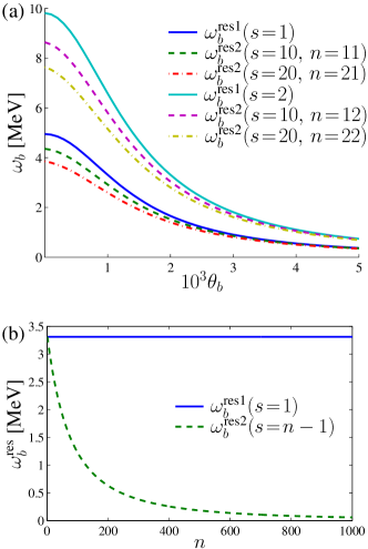
Figure 5: (Color online.) Panel (a) shows $\omega_{b}^{{\rm res}1}$ [Eq. (38)] and $\omega_{b}^{{\rm res}2}$ [Eq. (39)], as a function of $\theta_{b}$. Recall that we write $\bm{k}_{b}=\omega_{b}(\sin\theta_{b}\sin\psi_{b},\sin\theta_{b}\cos\psi_{b},\cos\theta_{b})$, i.e. $\theta_{b}$ is the angle between $\bm{k}_{b}$ and $\bm{p}_{i}$. The parameters employed are $\omega=2.5$ eV, $\xi=1$, $E_{i}=10^{3}m$, $\psi_{b}=\psi_{c}=0$, and $\theta_{c}=10^{-3}$. In panel (b), the resonance position of the first harmonic at $\theta_{b}=10^{-3}$ is plotted as a function of $n$. For $\omega_{b}^{{\rm res}1}$, the first harmonic (the resonance at lowest possible $\omega_{b}$) means $s=1$, and since for $\omega_{b}^{{\rm res}2}$ the value of $n-s$ tells us the order of the resonance, we have set $s=n-1$ for this curve. In fact, for large values of $n$, the resonance $\omega_{b}^{{\rm res}2}$ with $s=n-1$ shifts down to low photon energies, so that there will be resonances for any photon energy $\omega_{b}>0$. However, these higher-order resonances will be suppressed by a large-order Bessel function, and effectively, one can say that the higher-order resonances will not contribute provided $\xi$ is not too large ($\sim 1$).

II.5 Via gauge invariance to the differential rate

The matrix elements (26) and (31) are both invariant under the gauge transformations

$$\epsilon_{b}\to\epsilon_{b}+\lambda_{1}\,k_{b},\qquad\epsilon_{c}\to\epsilon_{c}+\lambda_{2}\,k_{c},$$ (40)

where $\lambda_{1,2}$ are arbitrary constants (that may depend on the parameters in the problem, i.e $\omega$, $q_{i}$ etc). This symmetry can be used for a numerical check of the computer code used for the evaluation, which we have performed in order to reassure ourselves regarding the consistency of the calculations. The gauge symmetry depends sensitively on the Bessel functions and the recurrence relations satisfied by them Lötstedt and Jentschura (2009b), so that all signs in the formulas have to be right for the symmetry to hold. The gauge symmetry can also be used to simplify the expression, for example, by gauge transforming so that terms proportional to $\epsilon_{b,c}\cdot\varkappa$ vanish. There is also invariance under the transformation $a\to a+\Lambda\varkappa$, $\Lambda$ constant, but since the four-vector $a$ always appears with a square, $a^{2}$, as $\hat{a}\hat{\varkappa}$, or in expressions like (LABEL:baralpha), this gauge symmetry is almost trivial and cannot be used as a meaningful validity check.

We now discuss how to obtain the differential two-photon rates, using the example of linear polarization. The differential rate per unit time $d\dot{W}$ is obtained as

$$d\dot{W}=\frac{1}{T}|S_{fi}|^{2}\frac{Vd^{3}q_{f}}{(2\pi)^{3}}\frac{Vd^{3}k_{b}}{(2\pi)^{3}}\frac{Vd^{3}k_{c}}{(2\pi)^{3}}.$$ (41)

Here, $d^{3}k_{b,c}=\omega_{b,c}^{2}d\omega_{b,c}d\Omega_{b,c}$. The squared amplitude $|S_{fi}|^{2}$ contains the Dirac $\delta$ of argument zero, $\left[\delta^{(4)}(0)\right]^{2}=\delta^{(4)}(q_{i}-q_{f}+n\varkappa-k_{b}-k_{c})TV(2\pi)^{-4}$, so that all factors of $V$ and $T$ in (41) cancel, as they should. We integrate over the final electron momentum and the photon energy $\omega_{c}$ with the delta function, and in addition we sum over the final electron spin (the final electron is always assumed to be unobserved), and average over the initial electron spin. Since in all examples we will present, the initial electron energy $E_{i}$ and laser intensity $\xi$ are chosen such that the quantum parameter $\chi$ [see Eq. (7)] is small, spin effects are marginal Ritus (1979). The final result then reads

$$\frac{d\dot{W}}{d\omega_{b}d\Omega_{b}d\Omega_{c}}=\;\sum_{r_{i},r_{f}=1}^{2}\sum_{n=1}^{\infty}\frac{e^{4}m^{2}\omega_{b}\omega_{c}^{2}}{8(2\pi)^{5}Q_{i}q_{f}\cdot k_{c}}$$ (42)

$$\;\times\left|\sum_{s=-\infty}^{\infty}\bar{u}_{r_{f}}(p_{f})\left[M_{b}^{s-n}\frac{\hat{{p}}_{b}+\frac{e^{2}a^{2}}{4k\cdot\tilde{p}_{b}}\hat{\varkappa}+m}{{p}_{b}^{2}-m_{\ast}^{2}}F_{b}^{s}\right.\right.$$

$$\left.\left.+{M}^{s-n}_{c}\frac{\hat{{p}}_{c}+\frac{e^{2}a^{2}}{4k\cdot{p}_{c}}\hat{\varkappa}+m}{{p}^{2}_{c}-m_{\ast}^{2}}{F}_{c}^{s}\right]u_{r_{i}}(p_{i})\right|^{2},$$

evaluated with $q_{f}=q_{i}+n\varkappa-k_{b}-k_{c}$ and $\omega_{c}$ is given by the first line of Eq. (II.4). Note also the factor $Q_{f}\omega_{c}/(q_{f}\cdot k_{c})$ arising from the delta function integration over $\omega_{c}$.

In order to obtain a well-defined expression for the differential rate close to the propagator poles (38), (39), it is necessary to discuss some kind of regularization procedure. One alternative is to include an imaginary correction to the mass and energy of the laser-dressed electron Becker and Mitter (1976); Schnez et al. (2007), so that $Q_{i}$ and $m$ in the propagator denominator are replaced according to

$$Q_{i}\to Q_{i}-i\frac{m\Gamma(\varkappa\cdot q_{i})}{2Q_{i}},\qquad m\to m-i\frac{\Gamma(\varkappa\cdot p_{b,c})}{2}.$$ (43)

The imaginary correction is related to the total rate for nonlinear single Compton scattering as $\Gamma(\varkappa\cdot q)=\frac{q^{0}}{m}\dot{W}_{\textrm{Compton}}$, and is given to a good approximation for small $\varkappa\cdot q/m^{2}$, $\xi=1$ and linear laser field polarization as $\Gamma(\varkappa\cdot q)=4\times 10^{-3}\varkappa\cdot q/m$ Schnez et al. (2007). The main problem with this regularization scheme is that the resulting scattering amplitude is not strictly gauge invariant, but the noninvariance induced by the small regularizing imaginary parts of the energies of the virtual states is moved to higher orders. We note that very similar questions concerning two-photon emission amplitudes for bound states have recently been discussed in Jentschura (2007, 2008); Jentschura and Surzhykov (2008); Jentschura (2009); Amaro et al. (2009). As an alternative, we propose to multiply the rate with the regularizing factor

$$\Phi=\prod_{s=-\infty}^{\infty}\left[1-{\rm e}^{-\frac{\tau}{m^{3}}\left(p_{b}^{2}-m_{\ast}^{2}\right)^{2}}\right]\left[1-{\rm e}^{-\frac{\tau}{m^{3}}\left(p_{c}^{2}-m_{\ast}^{2}\right)^{2}}\right],$$ (44)

where $\tau$ is the pulse length of the laser field. The rate is now proportional to $\tau$ at a resonance, and this way of regularizing is furthermore gauge invariant. Figure 6 shows an example of the differential rate (42), evaluated for a specific set of parameters corresponding to double Compton backscattering in a relativistically strong laser field. For $\omega_{b}\gtrapprox 2$ MeV, there is a “forest” of peaks at energies satisfying Eqs. (38) and (39). Note that according to Fig. 5 (b), the resonances $\omega^{\rm res2}_{b}(s=n-1)$ should actually lead to resonance peaks also at very low photon energies, but these are suppressed by large-order Bessel functions and thus not visible. The bright curves in Fig. 6 (c) correspond to the maxima in the differential rate induced by single-Compton scattering, but the rate is nonvanishing in other areas of the $\theta_{b}$-$\omega_{b}$-plane due to the two-photon emission.

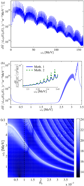
Figure 6: (Color online.) We illustrate the resonances of the fully differential rate (42) as a function of $\omega_{b}$. The parameters used are $\xi=1$, $E_{i}=10^{3}m$, $\epsilon_{b}=\epsilon_{b}^{1}$, $\epsilon_{c}=\epsilon_{c}^{1}$, $\theta_{c}=0.002$, $\psi_{b}=\psi_{c}=0$. In panels (a) and (b), a fixed value of $\theta_{b}=0.001$ is used, corresponding to a cut along the dashed line in (c). In panel (c), the color coding indicates the value of the decadic logarithm $\log_{10}\frac{d\dot{W}}{d\omega_{b}d\Omega_{b}d\Omega_{c}}$, where the argument of the logarithm is measured in units of s^-1sr^-2MeV^-1. The regularization method employed is given by a finite laser pulse duration as in Eq. (44), with $\tau=10^{4}/\omega$. In the inset of panel (b), both methods (43) [Meth. 1] and (44) [Meth. 2] are shown for comparison. For $\omega_{b}<2$ MeV, the application of the two methods yields numerically indistinguishable curves. The first Compton harmonic [the lowest bright curve in panel (c)] is broken at $\theta_{b}\approx 1.2\times 10^{-3}$, which can be understood as the point where $\bm{a}\cdot\bm{\epsilon}_{b}=0$ in the rest frame of the electron [in this frame, and in the gauge $\epsilon_{b}=(0,\bm{\epsilon}_{b})$, the Thomson cross section is proportional to $|\bm{a}\cdot\bm{\epsilon}_{b}|^{2}$].

The object of this paper is however not to study the behavior of the process close to the peaks, but rather to single out a kinematic region where unambiguous conclusions can be drawn independent of the method of regularization. The kinematic region best suited for such investigations seems to be for photon energies $\omega_{b}$ and angles $\theta_{b}$ smaller than some threshold such that the contribution from the cascade peaks are negligibly small. Mathematically, the suppression arises due to a large-order generalized Bessel functions (or, alternatively, ordinary Bessel functions in the case of circular laser polarization), which beyond some cutoff index decays exponentially with increasing $n$ Korsch et al. (2006); Lötstedt and Jentschura (2009b). In all subsequent examples in the remaining sections of this paper, we will therefore restrict the photon energy $\omega_{b}$ and the polar angle $\theta_{b}$ to the region $\omega_{b}\leq 1$ MeV and $\theta_{b}\leq 0.002$. Here, the result is independent of the method of regularization since we are sufficiently far away from the cascade peaks. With increasing $\xi$, the “safe” region shrinks, as the first Compton peak appears at lower energy $\omega_{b}$, see Eq. (38). Already at $\xi=2$, there are cascade contributions at $\omega_{b}\leq 1$ MeV, why we limit the laser intensity to $\xi\leq 1$ in the following.

III Comparison to perturbative double Compton scattering

In the limit $\xi\to 0$, the amplitudes (26), (31) reduce to the one found in Mandl and Skyrme (1952), where only one photon is absorbed from the laser. A discussion of this process can be found in standard textbooks Jauch and Rohrlich (1976), and was recently reexamined in Bell (2008). The above mentioned references as well as other previous works Ram and Wang (1971); Melrose (1972); Gould (1984) were devoted to the study of the cross section for unpolarized initial and final photons (with a few exceptions, see Carrassi and Passatore (1960); Radha and Thunga (1961)). However, as noted in Schützhold and Maia (2009), the discussion of photon polarization correlation necessitates an expression for the amplitude for arbitrary polarization of the final photons.

The amplitude $S^{PDCS}$ for perturbative double Compton scattering (PDCS) is given by the sum of the Feynman diagrams shown in Fig. 1, and reads Jauch and Rohrlich (1976)

$$S^{PDCS}= \frac{me^{3}(2\pi)^{4}}{\sqrt{8E_{i}E_{f}\omega\omega_{b}\omega_{c}V^{5}}}\delta(p_{f}+k_{b}+k_{c}-\varkappa-p_{i})$$

$$\times\left(\sum_{i=1}^{6}N_{i}\right),$$ (45)

where

$$\begin{split}N_{1}&=\bar{u}(p_{f})\hat{\epsilon}_{c}\frac{\hat{p}_{f}+\hat{k}_{c}+m}{(p_{f}+k_{c})^{2}-m^{2}}\hat{\epsilon}_{b}\frac{\hat{p}_{i}+\hat{\varkappa}+m}{(p_{i}+\varkappa)^{2}-m^{2}}\hat{\epsilon}u(p_{i}),\\ N_{2}&=\bar{u}(p_{f})\hat{\epsilon}_{c}\frac{\hat{p}_{f}+\hat{k}_{c}+m}{(p_{f}+k_{c})^{2}-m^{2}}\hat{\epsilon}\frac{\hat{p}_{i}-\hat{k}_{b}+m}{(p_{i}-k_{b})^{2}-m^{2}}\hat{\epsilon}_{b}u(p_{i}),\\ N_{3}&=\bar{u}(p_{f})\hat{\epsilon}\frac{\hat{p}_{f}-\hat{\varkappa}+m}{(p_{f}-\varkappa)^{2}-m^{2}}\hat{\epsilon}_{c}\frac{\hat{p}_{i}-\hat{k}_{b}+m}{(p_{i}-k_{b})^{2}-m^{2}}\hat{\epsilon}_{b}u(p_{i})\,,\end{split}$$ (46)

$N_{4}=N_{1}(b\leftrightarrow c)$, $N_{5}=N_{2}(b\leftrightarrow c)$ and $N_{6}=N_{3}(b\leftrightarrow c)$ in a self-explanatory notation. Here, $\epsilon$ represents the polarization vector of the laser field. The rate is then

$$d\dot{W}=J\left|S^{PDCS}\right|^{2}\frac{1}{T}V\frac{Vd^{3}k_{b}}{(2\pi)^{3}}\frac{Vd^{3}k_{c}}{(2\pi)^{3}}\frac{Vd^{3}p_{f}}{(2\pi)^{3}}$$ (47)

$$=\frac{\xi^{2}m^{4}e^{4}}{8E_{i}E_{f}\omega_{b}\omega_{c}(2\pi)^{5}}\left|\sum_{i=1}^{6}N_{i}\right|^{2}\delta(p_{f}+k_{b}+k_{c}-p_{i}-\varkappa)d^{3}k_{b}d^{3}k_{c}d^{3}p_{f},$$

where $J=\frac{\omega m^{2}\xi^{2}}{e^{2}}$ is the photon flux. Integrating over $d^{3}p_{f}$ and $d\omega_{c}$, and summing and averaging over the electron spin, we obtain

$$\frac{d\dot{W}^{PDCS}}{d\omega_{b}d\Omega_{b}d\Omega_{c}}=\xi^{2}\frac{m^{4}e^{4}\omega_{b}\omega_{c}^{2}}{16(2\pi)^{5}E_{i}p_{f}\cdot k_{c}}\sum_{r_{i},r_{f}=1}^{2}\left|\sum_{j=1}^{6}N_{j}\right|^{2}.$$ (48)

The dependence on $\xi$ is thus given by the prefactor $\xi^{2}$, and we may thus refer to this process as the “linear” process because the rate is proportional to the laser intensity.

In Figs. 7 and 8, we show a comparison of the predictions of the nonperturbative formulas [Eq. (26) and Eq. (31)] and the perturbative formula [(III)] for the differential rate, for both circular and linear polarization of the laser field. Note that to compare with the circular polarization, one should put $\epsilon=(0,1,i,0)/\sqrt{2}$ in Eq. (46). The figures show that the photons may be produced in any polarization state, although parallel polarization of the two emitted photons $\epsilon_{b}\cdot\epsilon_{c}\approx 1$ is the dominant channel for linear laser polarization. Due to the rotational symmetry, circular laser polarization results in similar differential rates for both parallel and perpendicular polarization of the emitted high-energy photons [see Figs. 7(d)–(f) and (j)–(l)]. For small laser intensity, the plane defined by the polarization and propagation axes of the laser characterizes the emission pattern of the accelerated charge, so that alignment of the two emitted photons as shown in the third row of Fig. 7 can be expected. Our numerical results show that this intuitive picture is still valid in the relativistic, nonperturbative laser interaction regime, although some details change: e.g., the emission of photons with antiparallel polarization vectors is favored over the parallel case, as is evident from the first panel in the upper row of Fig. 7. We here recall that the direction of the polarization basis vectors $\epsilon_{b,c}^{1,2}$ depends on the angles $\psi_{b,c}$, see Fig. 3. Figure 8 confirms this picture, here the difference of the differential rate between the parallel case ($\epsilon_{b}\cdot\epsilon_{c}\approx 1$) and the perpendicular case ($\epsilon_{b}\cdot\epsilon_{c}\approx 0$) amounts to several orders of magnitude.

In order to demonstrate the contribution from the different photon orders $n$, we refer to Fig. 9. Here the dependence on the photon order $n$ is shown, if we define

$$\frac{d\dot{W}}{d\omega_{b}d\Omega_{b}d\Omega_{c}}=\sum_{n=1}^{\infty}\frac{d\dot{W}^{n}}{d\omega_{b}d\Omega_{b}d\Omega_{c}}.$$ (49)

As can be seen from Fig. 9, typically up to 20 photons contribute to the differential rate. Equation (II.4) for $n\leq 20$ then yields $\omega_{c}\leq 70$ MeV, which implies that even though the “first” photon has modest energy $\omega_{b}=1$ MeV, the energy of the “second” photon is much larger. The difference between the smooth curve in the circular case and the sawtooth shape of the linear curve can be traced back to the behavior of the generalized Bessel function and the usual Bessel function, constituting the amplitudes (26) and (31). For example, for the parameters shown in Fig. 9(b), one can show that the dominant contribution to the matrix element for linear polarization is roughly proportional to the generalized Bessel function $A_{1}(n,0,\beta)$, which vanishes for even $n$ Lötstedt and Jentschura (2009b). However, if the polarization vectors are summed over, then the case of even $n$ contributes, and the curve smoothens out. Similar selection rules for the emitted harmonics occur also for the nonlinear single Compton scattering process Ritus (1979). On the contrary, the circular polarization curve is smooth due to the rotational symmetry.

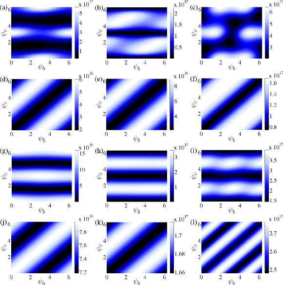
Figure 7: (Color online.) Contour plot of the differential rate for different final photon polarizations. The color coding indicates the value of the differential rate $\frac{d\dot{W}}{d\omega_{b}d\Omega_{b}d\Omega_{c}}$, on linear scale, in units of s^-1sr^-2MeV^-1. The upper two rows [(a)–(f)] display the result of the nonperturbative formula, and the lower two rows [(g)–(l)] show the perturbative results. The parameters used are $\xi=1$, $\omega=2.5$ eV, $E_{i}=10^{3}m$, $\omega_{b}=1$ MeV, and $\theta_{b}=2\theta_{c}=10^{-3}$. In this case, $\omega_{c}$ is fixed by the scattering geometry but still depends on the number $n$ of exchanged photons; we present the differential rate summed over all $n$ and thus suppose that the energy $\omega_{c}$ is unobserved. For the polarizations, we have linear laser polarization in (a)–(c) and (g)–(i) (first and third row), and circular laser polarization in (d)–(f) and (j)–(l) (second and fourth row). In (a), (d), (g), and (j) (first column) we have $\epsilon_{b}=\epsilon_{b}^{1}$, $\epsilon_{c}=\epsilon_{c}^{1}$, where we recall that the polarization vectors are defined in Eq. (II.1). In (b), (e), (h), and (k) (middle column) we have $\epsilon_{b}=\epsilon_{b}^{1}$, $\epsilon_{c}=\epsilon_{c}^{2}$, and panels (c), (f), (i) and (l) (right column) show the differential rate summed over all possible polarizations of the final photons.

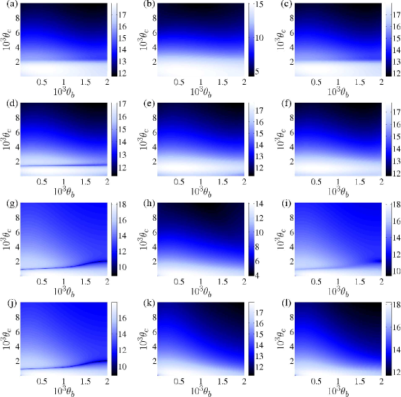
Figure 8: (Color online.) Contour plot of the differential rate as a function of the polar angles $\theta_{b}$ and $\theta_{c}$. The color coding indicates the value of the decadic logarithm $\log_{10}\frac{d\dot{W}}{d\omega_{b}d\Omega_{b}d\Omega_{c}}$, with the differential rate given in units of s^-1sr^-2MeV^-1. As in Fig. 7, the upper two rows [(a)–(f)] show nonperturbative, and the lower two rows [(g)–(l)] perturbative results, respectively. The parameters used are $\xi=1$, $\omega=2.5$ eV, $E_{i}=10^{3}m$, $\omega_{b}=1$ MeV, and $\psi_{b}=0$, $\psi_{c}=\pi$. For the polarizations, we have linear laser polarization in (a)–(c) and (g)–(i) (first and third row), and circular laser polarization in (d)–(e) and (j)–(l) (second and fourth row). In (a), (d), (g), and (j) (left column) we have $\epsilon_{b}=\epsilon_{b}^{1}$, $\epsilon_{c}=\epsilon_{c}^{1}$, In (b), (e), (h), and (k) (middle column) we have $\epsilon_{b}=\epsilon_{b}^{1}$, $\epsilon_{c}=\epsilon_{c}^{2}$, and panels (c), (f), (i) and (l) (right column) show the differential rate summed over the final photon polarizations. Note that from Fig. 3, we have $\epsilon^{1}_{b}\cdot\epsilon^{1}_{c}\approx 1$ and $\epsilon^{1}_{b}\cdot\epsilon^{2}_{c}\approx 0$ here.

Figure 9: (Color online.) Demonstration of the multiphoton character of the pair creation rate, for linear and circular polarization of the laser field. In (a), $\psi_{b}=0$, $\psi_{c}=\pi$, and the final polarization is fixed to $\epsilon_{b}=\epsilon_{b}^{1}$, $\epsilon_{c}=\epsilon_{c}^{1}$, while in (b) we have $\psi_{b}=\pi/2$, $\psi_{c}=3\pi/2$, and $\epsilon_{b}=\epsilon_{b}^{1}$, $\epsilon_{c}=\epsilon_{c}^{2}$. Otherwise the parameters are the same as in Fig. 7.

To conclude this section, we investigate if the integrated rate differ in the perturbative and nonperturbative case. In Fig. 10, we show, as a function of $\xi$, the quantity

$$\begin{split}\dot{W}_{\textrm{int}}={}&\sum_{\lambda_{b},\lambda_{c}}\int\limits_{0}^{2\pi}d\psi_{b}\int\limits_{0}^{2\pi}d\psi_{c}\int\limits_{0}^{\theta_{b,\textrm{max}}}\sin{\theta_{b}}d\theta_{b}\\ &\times\int\limits_{0}^{\theta_{c,\textrm{max}}}\sin{\theta_{c}}d\theta_{c}\int\limits_{\omega_{b,\textrm{min}}}^{\omega_{b,\textrm{max}}}d\omega_{b}\,\frac{d\dot{W}}{d\omega_{b}d\Omega_{b}d\Omega_{c}},\end{split}$$ (50)

with $\theta_{b,\textrm{max}}=1.5\times 10^{-3}$, $\theta_{c,\textrm{max}}=2.5\times 10^{-3}$, $\omega_{b,\textrm{min}}=10^{-3}$ MeV, and $\omega_{b,\textrm{max}}=1$ MeV. This restriction is identical to the one in Lötstedt and Jentschura (2009a). By restricting the final phase space, one can ensure that contributions from the single Compton scattering cascade are negligible, as discussed in Sec. II.5. Figure 10 reveals that the integrated rate is slightly larger than one would expect from the perturbative formula, and also that circular and linear polarization of the laser gives almost identical results, despite their different angular characteristics (see Figs. 7, 8). Another remark is that for the integrated rate, the perturbative formula gives identical results regardless of laser polarization because interference terms in the expanded perturbative rate vanish after the integration. In the interval considered ($\xi<1$), the relative difference of the integrated nonperturbative and the integrated perturbative rate can be approximately fitted to a power law as $\dot{W}_{\textrm{int}}^{\textrm{nonpert}}-\dot{W}_{\textrm{int}}^{\textrm{pert}}\propto\xi^{\eta}$, with $\eta\approx 2.7$ for linear and $\eta\approx 3$ for circular laser polarization, respectively.

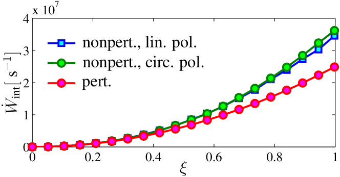
Figure 10: (Color online.) The integrated rate (50), defined in Eq. (50) for $\omega=2.5$ eV and $E_{i}=10^{3}m$. The figure compares the nonperturbative formula for linear laser polarization [Eq. (42)], for circular laser polarization [Eq. (31)], and the perturbative expression [Eq. (48)].

IV Angular correlation and entanglement

We now turn our attention to the important questions regarding the quantum mechanical correlation, i.e. entanglement, of the two final photons. The theory we apply in this section have been previously used extensively to characterize the final-state correlation in bound states transitions Radtke et al. (2006, 2008a, 2008b); Maiorova et al. (2009). The idea is to use the information contained in the matrix elements (26), (31), to obtain an expression for the density matrix $\rho_{f}$ of the polarizations of the final system “electron+two photons”. Given an expression for $\rho_{f}$, it is then straightforward to calculate the concurrence Wootters (1998), which is a measurement of how much the two photons are entangled. The starting point is the initial density matrix Blum (1996)

$$\rho_{i}=\sum_{r_{i}=1}^{2}|r_{i},0,0\rangle\langle r_{i},0,0|,$$ (51)

where $r_{i}$ is the spin of the initial electron and the zeros denote the absence of photons (other than laser photons of course) in the initial state. The initial electron is thus assumed to be unpolarized. Note also that all dependencies on energies and angles etc of the state vectors are not written out. Next, due to the interaction $R$, the density matrix $\rho_{i}$ evolves into the final state density matrix $\rho_{f}$,

$$\rho_{f}=R\rho_{i}R^{\dagger}=\sum_{r_{i}=1}^{2}R|r_{i},0,0\rangle\langle r_{i},0,0|R^{\dagger}.$$ (52)

The matrix elements of $\rho_{f}$ are thus given by

$$\langle r_{f},\lambda_{b},\lambda_{c}|\rho_{f}|r^{\prime}_{f},\lambda^{\prime}_{b},\lambda^{\prime}_{c}\rangle$$

$$=\sum_{r_{i}=1}^{2}\langle r_{f},\lambda_{b},\lambda_{c}|R|r_{i},0,0\rangle\langle r_{i},0,0|R^{\dagger}|r^{\prime}_{f},\lambda^{\prime}_{b},\lambda^{\prime}_{c}\rangle,$$ (53)

where $\lambda_{b,c}$, $\lambda^{\prime}_{b,c}\in\{1,2\}$ denotes the polarization components of the emitted photons in either Cartesian or circular basis. If the final electron is unobserved, we should trace out $r_{f}$:

$$\langle\lambda_{b},\lambda_{c}|\rho_{f}|\lambda^{\prime}_{b},\lambda^{\prime}_{c}\rangle$$

$$=\sum_{r_{i},r_{f}=1}^{2}\langle r_{f},\lambda_{b},\lambda_{c}|R|r_{i},0,0\rangle\,\langle r_{i},0,0|R^{\dagger}|r_{f},\lambda^{\prime}_{b},\lambda^{\prime}_{c}\rangle.$$ (54)

If we now identify

$$\langle r_{f},\lambda_{b},\lambda_{c}|R|r_{i},0,0\rangle= \;\sqrt{N}S_{fi}(r_{i},r_{f},\lambda_{b},\lambda_{c}),$$

$$\langle r_{i},0,0|R^{\dagger}|r_{f},\lambda^{\prime}_{b},\lambda^{\prime}_{c}\rangle= \;\sqrt{N}S_{fi}^{\ast}(r_{i},r_{f},\lambda^{\prime}_{b},\lambda^{\prime}_{c}),$$ (55)

where $N$ is a normalization constant, and we use the explicit basis

$$\begin{split}|1\;1\rangle&=\binom{1}{0}\otimes\binom{1}{0}=\left(\begin{array}[]{c}1\\ 0\\ 0\\ 0\end{array}\right),\\ |1\;2\rangle&=\binom{1}{0}\otimes\binom{0}{1}=\left(\begin{array}[]{c}0\\ 1\\ 0\\ 0\end{array}\right),\\ |2\;1\rangle&=\binom{0}{1}\otimes\binom{1}{0}=\left(\begin{array}[]{c}0\\ 0\\ 1\\ 0\end{array}\right),\\ |2\;2\rangle&=\binom{0}{1}\otimes\binom{0}{1}=\left(\begin{array}[]{c}0\\ 0\\ 0\\ 1\end{array}\right),\end{split}$$ (56)

for the polarization state of the final photons, then the expression for the final density $4\times 4$ matrix reads

$$\rho_{f}=\sum_{r_{i},r_{f}=1}^{2}N\left(\begin{array}[]{cccc}S_{11}S_{11}^{\ast}&S_{11}S_{12}^{\ast}&S_{11}S_{21}^{\ast}&S_{11}S_{22}^{\ast}\\ S_{12}S_{11}^{\ast}&S_{12}S_{12}^{\ast}&S_{12}S_{21}^{\ast}&S_{12}S_{22}^{\ast}\\ S_{21}S_{11}^{\ast}&S_{21}S_{12}^{\ast}&S_{21}S_{21}^{\ast}&S_{21}S_{22}^{\ast}\\ S_{22}S_{11}^{\ast}&S_{22}S_{12}^{\ast}&S_{22}S_{21}^{\ast}&S_{22}S_{22}^{\ast}\end{array}\right),$$ (57)

where

$$S_{\lambda_{b}\lambda_{c}}=S_{fi}(r_{i},r_{f},\lambda_{b},\lambda_{c}).$$ (58)

The normalization constant $N$ can be found by requiring

$$1=\textrm{Tr}\rho_{f}=\sum_{r_{i},r_{f}}N\left(|S_{11}|^{2}+|S_{12}|^{2}+|S_{21}|^{2}+|S_{22}|^{2}\right).$$ (59)

According to Wootters (1998), the concurrence $C(\rho_{f})$ is now given by

$$C(\rho_{f})=\textrm{max}(0,\sqrt{\zeta_{1}}-\sqrt{\zeta_{2}}-\sqrt{\zeta_{3}}-\sqrt{\zeta_{4}}),$$ (60)

where the $\zeta_{j}$’s are the eigenvalues, in descending order, of the matrix

$$Q=\rho_{f}\left(\sigma^{2}\otimes\sigma^{2}\right)\rho_{f}^{\ast}\left(\sigma^{2}\otimes\sigma^{2}\right),$$ (61)

where $\sigma^{2}$ is the second Pauli spin matrix. The eigenvalues $\zeta_{j}$ are real and positive. The concurrence as defined in Eq. (60) is gauge invariant, and does not depend on the basis used for the polarization vectors of the photons, i.e. either the Cartesian basis, Eq. (II.1), or the helicity basis, Eq. (25), can be used. An explicit expression for $\left(\sigma^{2}\otimes\sigma^{2}\right)$ as a $4\times 4$ matrix is given by

$$\left(\sigma^{2}\otimes\sigma^{2}\right)=\left(\begin{array}[]{cc}0&-i\\ i&0\end{array}\right)\otimes\left(\begin{array}[]{cc}0&-i\\ i&0\end{array}\right)=\left(\begin{array}[]{cccc}0&0&0&-1\\ 0&0&1&0\\ 0&1&0&0\\ -1&0&0&0\end{array}\right).$$ (62)

The matrix $\left(\sigma^{2}\otimes\sigma^{2}\right)$ is a kind of spin-flip operator for qubits, we have

$$\begin{split}\left(\sigma^{2}\otimes\sigma^{2}\right)|1\;1\rangle=-|2\;2\rangle,&\quad\left(\sigma^{2}\otimes\sigma^{2}\right)|2\;2\rangle=-|1\;1\rangle,\\ \left(\sigma^{2}\otimes\sigma^{2}\right)|1\;2\rangle=|2\;1\rangle,&\quad\left(\sigma^{2}\otimes\sigma^{2}\right)|2\;1\rangle=|1\;2\rangle.\end{split}$$ (63)

This means that a maximally entangled pure state is an eigenstate of $\left(\sigma^{2}\otimes\sigma^{2}\right)$:

$$\left(\sigma^{2}\otimes\sigma^{2}\right)\left(|1\;2\rangle-|2\;1\rangle\right)=-|1\;2\rangle+|2\;1\rangle,$$ (64)

and consequently has unity concurrence.

We now provide some examples and compare the concurrence (60) for different laser polarizations and furthermore show that the nonperturbative treatment is indispensable to correctly predict the degree of correlation. Figure 11 shows the concurrence as a function of the azimuth angles $\psi_{b}$, $\psi_{c}$. This figure should be compared to Fig. 7. In Fig. 12, we show instead the dependence on the polar angles $\theta_{b,c}$, which should be compared with the corresponding Fig. 8 for the differential rate.

We remark that to be able to measure the concurrence, it is desirable to find angular regions where high concurrence and high differential rate overlap. This seems to be possible, at least in some cases: e.g., one may compare Fig. 12(c) with Fig. 8(l). Moreover, the general trend is that a strong laser field diminishes the concurrence. Therefore, if high entanglement is sought, it is advisable to employ a perturbative laser beam ($\xi<1$), although the nonperturbative dependence of the concurrence as a function of $\xi$ would be highly interesting to measure. Similar conclusions as those above follow from the previous investigation Lötstedt and Jentschura (2009a). A final remark is that linear and circular laser polarization are seen to lead to similar peak values of the concurrence.

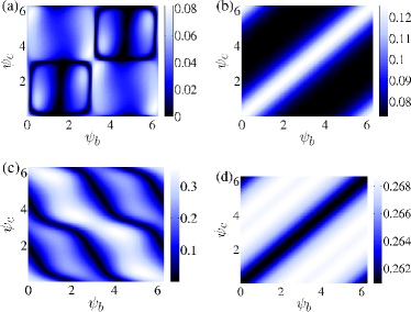
Figure 11: (Color online.) Contour plot of concurrence as a function of the azimuth angles $\psi_{b}$ and $\psi_{c}$. The color coding indicates the value of the concurrence $C(\rho_{f})$ [see Eq. (60)]. Panel (a) shows linear laser polarization, and (b) circular laser polarization, both calculated with the nonperturbative expressions for the amplitude. The results of the perturbative formula are displayed in panel (c) [linear laser polarization] and (d) [circular laser polarization]. The values of $E_{i}$, $\omega$, $\xi$ and $\theta_{b,c}$ are the same as in Fig. 7.

Figure 12: (Color online.) Contour plot of concurrence as a function of the polar angles $\theta_{b}$ and $\theta_{c}$. The color coding indicates the value of the concurrence $C(\rho_{f})$ [see Eq. (60)]. Panel (a): linear laser polarization, nonperturbative, (b): circular laser polarization, nonperturbative, (c): linear laser polarization, perturbative, (d): circular laser polarization, perturbative. Laser parameters as well as the initial electron energy $E_{i}$ and the photon azimuth angles $\psi_{b,c}$ are the same as in Fig. 8.

V Conclusions

Our treatment of double Compton scattering in intense laser fields in based on the canonical formalism of Furry-picture quantum electrodynamics (QED), where a strong external field (in this case, the oscillatory laser field) is incorporated into the fermion propagators. The oscillatory nature of the laser field necessitates the expansion of all initial and final fermion states into plane waves, thereby giving rise to generalized (linear polarization) and ordinary (circular polarization) Bessel functions. The formalism, as outlined in Sec. II, leads to a consistent formulation of the nonperturbative double Compton scattering for an arbitrary intensity of the laser field, and with full account of all relativistic and spin-dependent effects on the electron lines. In particular, a suitable generalization of the formalism outlined here would apply to three-photon events, which can be described by a third-order amplitude in QED.

In addition to a consistent formulation of the polarization resolved production rates, differential in the photon emission angles and energy, for two-photon transitions of Dirac–Volkov states in intense laser fields, we numerically show that only a fully relativistic formalism, nonperturbative in the laser field strength, can possibly yield experimentally verifiable, consistent predictions. This is not surprising because the differential rates depend crucially on details of the emission process, which in turn is highly dependent on the properties of the propagators near the resonances. Indeed, it is possible to identify those angular and photon energy regions where only the two-photon amplitude, not the single-Compton resonances, give appreciable contributions to the photon emission, and it is thus possible to observe entangled high-energy photons in coincidence without having to worry about background from resonant cascade emission by single-photon transitions.

The necessity of the nonperturbative formalism is demonstrated in Sec. III. The perturbative (in the laser field interaction) double Compton scattering cannot give reliable predictions if the nonlinear intensity parameter $\xi$ approaches unity. We stress that a value $\xi\approx 1$, corresponding to laser intensities of the order of $10^{18}$ W/cm² for optical lasers, is routinely available today in many laboratories worldwide. In Figs. 7 and 8, we show that depending on polarization and the observation solid angle, even order-of-magnitude differences can exist between the rates evaluated with the nonperturbative and the perturbative formulas. However, if angles and photon energies are integrated over, the results are similar, as shown in Fig. 10, although the difference grows nonlinearly with $\xi$, illustrating the importance of higher orders.

The polarization entanglement is interesting but needs to be quantified. Therefore, we discuss, in Sec. IV, the concurrence as a gauge-independent measure of the photon entanglement. Our results (see Figs. 11 and 12) indicate that close to maximally entangled (unity concurrence) photon pairs may be produced, but only in certain angular regions. Furthermore, the degree of entanglement changes strongly with the laser field intensity. An experimental verification of the entanglement would yield a test for this fundamental quantum phenomenon in a high-energy domain where it is otherwise difficult to generate entangled quanta.

Finally, we remark that the two-photon emission is not a “rare” or “unusual” physical process but a simple generalization of the basic physical phenomenon of radiation emission by moving charges, and that, therefore, we can assume that experimental access in the near future is entirely realistic.

References

• Eliezer (1946) C. J. Eliezer, Proc. Roy. Soc. (London) A187, 210 (1946).
• Mandl and Skyrme (1952) F. Mandl and T. H. R. Skyrme, Proc. Roy. Soc. London A 215, 497 (1952).
• Bell (2008) F. Bell, eprint eprint arXiv:0809.1505v1 [quant-ph].
• Cavanagh (1952) P. E. Cavanagh, Phys. Rev. 87, 1131 (1952).
• Theus and Beach (1957) R. B. Theus and L. A. Beach, Phys. Rev. 106, 1249 (1957).
• McGie et al. (1966) M. R. McGie, F. P. Brady, and W. J. Knox, Phys. Rev. 152, 1190 (1966).
• Sekhon et al. (1988) G. S. Sekhon, B. S. Sandhu, and B. S. Ghumman, Physica C 150, 473 (1988).
• Sandhu et al. (1999) B. S. Sandhu, R. Dewan, B. Singh, and B. S. Ghumman, Phys. Rev. A 60, 4600 (1999).
• Saddi et al. (2006) M. B. Saddi, B. S. Sandhu, and B. Singh, Ann. Nucl. Ener. 33, 271 (2006).
• Saddi et al. (2008) M. B. Saddi, B. Sing, and B. S. Sandhu, Nucl. Instrum. Meth. B 266, 3309 (2008).
• Melrose (1972) D. B. Melrose, Nuov. Cim. 7 A, 669 (1972).
• Lötstedt et al. (2007) E. Lötstedt, U. D. Jentschura, and C. H. Keitel, Phys. Rev. Lett. 98, 043002 (2007).
• Reiss and Eberly (1966) H. R. Reiss and J. H. Eberly, Phys. Rev. 151, 1058 (1966).
• Brodin et al. (2008) G. Brodin, M. Marklund, R. Bingham, J. Collier, and R. G. Evans, Class. Quantum Grav. 25, 145005 (2008).
• Thirolf et al. (2009) P. G. Thirolf, D. Habs, A. Henig, D. Jung, D. Kiefer, C. Lang, J. Schreiber, C. Maia, G. Schaller, R. Schützhold, et al., Eur. Phys. J. D 55, 379 (2009).
• Schützhold et al. (2006) R. Schützhold, G. Schaller, and D. Habs, Phys. Rev. Lett. 97, 121302 (2006).
• Schützhold et al. (2008) R. Schützhold, G. Schaller, and D. Habs, Phys. Rev. Lett. 100, 091301 (2008).
• Schützhold and Maia (2009) R. Schützhold and C. Maia, Eur. Phys. J. D 55, 375 (2009).
• Wootters (1998) W. K. Wootters, Phys. Rev. Lett. 80, 2245 (1998).
• Cirone (2005) M. A. Cirone, Phys. Lett. A 339, 269 (2005).
• Baier et al. (1981) V. N. Baier, V. S. Fadin, V. A. Khoze, and E. A. Kuraev, Phys. Rep. 78, 293 (1981).
• Altman and Quarles (1985) J. C. Altman and C. A. Quarles, Phys. Rev. A 31, R2744 (1985).
• Véniard et al. (1987) V. Véniard, M. Gavrila, and A. Maquet, Phys. Rev. A 35, R448 (1987).
• Hippler (1991) R. Hippler, Phys. Rev. Lett. 66, 2197 (1991).
• Kahler et al. (1992) D. L. Kahler, J. Liu, and C. A. Quarles, Phys. Rev. Lett. 68, 1690 (1992).
• Korol (1997) A. V. Korol, J. Phys. B 30, 413 (1997).
• Dondera and Florescu (1998) M. Dondera and V. Florescu, Phys. Rev. A 58, 2016 (1998).
• Krylovetskiĭ et al. (2002) A. A. Krylovetskiĭ, N. L. Manakov, S. I. Marmo, and A. F. Starace, Zh. Éksp. Teor. Fiz. 122, 1168 (2002), [JETP 95, 1006 (2002)].
• Korol and Solovjev (2006) A. V. Korol and I. A. Solovjev, Rad. Phys. Chem. 75, 1346 (2006).
• Zhukovskiĭ and Nikitina (1973) V. C. Zhukovskiĭ and N. S. Nikitina, Zh. Éksp. Teor. Fiz. 64, 1169 (1973), [Sov. Phys.-JETP 37, 595 (1973)].
• Sokolov et al. (1976) A. A. Sokolov, A. M. Voloshchenko, V. C. Zhukovskii, and Yu. G. Pavlenko, Izv. Vyssh. Uchebn. Zaved., Fiz. 19, 46 (1976), [Rus. Phys. J. 19, 1139 (1976)].
• Fomin and Kholodov (2003) P. I. Fomin and R. I. Kholodov, Zh. Éksp. Teor. Fiz. 123, 356 (2003), [JETP 96, 315 (2003)].
• Morozov and Ritus (1975) D. A. Morozov and V. I. Ritus, Nucl. Phys. B 86, 309 (1975).
• Lötstedt and Jentschura (2009a) E. Lötstedt and U. D. Jentschura, Phys. Rev. Lett. 103, 110404 (2009).
• Ritus (1979) V. I. Ritus, Trud. Ord. Len. Fiz. Inst. im. P. N. Leb. Akad. Nauk SSSR 111, 5 (1979), [J. Rus. Laser Res. 6, 497 (1985)].
• Reiss (1962) H. R. Reiss, J. Math. Phys. 3, 59 (1962).
• Korsch et al. (2006) H. J. Korsch, A. Klumpp, and D. Witthaut, J. Phys. A 39, 14947 (2006).
• Roshchupkin (1985) S. P. Roshchupkin, Yad. Fiz. 41, 1244 (1985), [Sov. J. Nucl. Phys. 41, 796 (1985)].
• Nikishov and Ritus (1964) A. I. Nikishov and V. I. Ritus, Zh. Éksp. Teor. Fiz. 46, 776 (1964), [Sov. Phys. JETP 19, 529 (1964)].
• Harvey et al. (2009) C. Harvey, T. Heinzl, and A. Ilderton, Phys. Rev. A 79, 063407 (2009).
• Panek et al. (2002) P. Panek, J. Z. Kamiński, and F. Ehlotzky, Phys. Rev. A 65, 022712 (2002).
• Bamber et al. (1999) C. Bamber, S. J. Boege, T. Koffas, T. Kotseroglou, A. C. Melissinos, D. D. Meyerhofer, D. A. Reis, W. Ragg, C. Bula, K. T. McDonald, et al., Phys. Rev. D 60, 092004 (1999).
• Lötstedt and Jentschura (2009b) E. Lötstedt and U. D. Jentschura, Phys. Rev. E 79, 026707 (2009b).
• Becker and Mitter (1976) W. Becker and H. Mitter, J. Phys. A 9, 2171 (1976).
• Schnez et al. (2007) S. Schnez, E. Lötstedt, U. D. Jentschura, and C. H. Keitel, Phys. Rev. A 75, 053412 (2007).
• Jentschura and Surzhykov (2008) U. D. Jentschura and A. Surzhykov, Phys. Rev. A 77, 042507 (2008).
• Jentschura (2007) U. D. Jentschura, J. Phys. A 40, F223 (2007).
• Jentschura (2008) U. D. Jentschura, J. Phys. A 41, 155307 (2008).
• Jentschura (2009) U. D. Jentschura, Phys. Rev. A 79, 022510 (2009).
• Amaro et al. (2009) P. Amaro, J. P. Santos, F. Parente, A. Surzhykov, and P. Indelicato, Phys. Rev. A 79, 062504 (2009).
• Jauch and Rohrlich (1976) J. M. Jauch and F. Rohrlich, The theory of photons and electrons (Addison-Wesley publishing company, Reading, Massachusetts, 1976), 2nd ed.
• Ram and Wang (1971) M. Ram and P. Y. Wang, Phys. Rev. Lett. 26, 476 (1971); erratum: Phys. Rev. Lett. 26, 1210 (1971).
• Gould (1984) R. J. Gould, Astrophysical J. 285, 275 (1984).
• Radha and Thunga (1961) T. K. Radha and R. Thunga, Z. Phys. 161, 20 (1961).
• Carrassi and Passatore (1960) M. Carrassi and G. Passatore, Nuov. Cim. 16, 1835 (1960).
• Radtke et al. (2008a) T. Radtke, A. Surzhykov, and S. Fritzsche, Phys. Rev. A 77, 022507 (2008a).
• Radtke et al. (2008b) T. Radtke, A. Surzhykov, and S. Fritzsche, Eur. Phys. J. D 49, 7 (2008b).
• Maiorova et al. (2009) A. V. Maiorova, A. Surzhykov, S. Tashenov, V. M. Shabaev, S. Fritzsche, G. Plunien, and T. Stöhlker, J. Phys. B 42, 125003 (2009).
• Radtke et al. (2006) T. Radtke, S. Fritzsche, and A. Surzhykov, Phys. Rev. A 74, 032709 (2006).
• Blum (1996) K. Blum, Density matrix theory and applications (Plenum Press, New York, 1996), 2nd ed.