STIMULATED RAMAN ADIABATIC PASSAGE
IN THE FIELD OF FINITE DURATION PULSES

Abstract

The theory of stimulated Raman adiabatic passage in a three-level $\Lambda$-scheme of the interaction of an atom or molecule with light, which takes the nonadiabatic processes at the beginning and the end of light pulses into account, is developed.

I Introduction

Adiabatic processes in atomic physics, owing to their stability with respect to a variation of parameters that describe the interaction with a field, play an especial role as a tool for manipulating atomic and molecular states. For instance, a fast adiabatic passage of the light pulse carrier frequency through the resonance with the atomic transition frequency allows one to obtain an atom or molecule in the excited state with a probability close to 1 Sho90 ; Sho08 . In this work, we study the stimulated Raman adiabatic passage (STIRAP), which can be realized in a three- and a multilevel scheme of the interaction between the atom and the field and was predicted as early as in the 1980s Ore84 ; Gau88 . The physical aspects and numerous applications of STIRAP in various branches of physics and chemistry are discussed in reviews Ber98 ; Vit01 and in work Sho08 . Recently, STIRAP has been demonstrated to occur in solids Got06 .

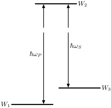
Figure 1: Scheme of the atom-field interaction. A Stokes pulse with the carrier frequency $\omega_{S}$ affects the atom firstly and is followed by the second pumping pulse with the carrier frequency $\omega_{P}$, by partially overlapping in time with the first pulse. Here, $W_{1}$, $W_{2}$, and $W_{3}$ are the energies of atomic states $\left|1\right\rangle$, $\left|2\right\rangle$, and $\left|3\right\rangle$, respectively

STIRAP is based on the existence of a trapped or “dark” state which arises provided that there is a two-photon resonance between an atom (in what follows, when speaking about an atom, we also mean a molecule) and a radiation field produced by two lasers Alz76 ; Ari76 ; Gra78 . In the simplest case considered in this work, the laser carrier frequencies are so selected that they are close to the frequency of the transition between the excited state and two states with lower energies–both metastable or stable and metastable ones (the three-level $\Lambda$-scheme of the interaction between the atom and laser radiation). The radiation of one of the lasers – the pumping field – couples states $\left|1\right\rangle$ and $\left|2\right\rangle$ (see Fig. 1). The field of the other laser – the Stokes field – couples states $\left|3\right\rangle$ and $\left|2\right\rangle$. The difference between the frequencies of those fields coincides with the transition frequency $\left|1\right\rangle\leftrightarrow\left|3\right\rangle$. In this case, some time after the interaction of the atom with the field has started, the probability to find the atom in the excited state $\left|2\right\rangle$ is close to zero, i.e. the atomic state is described by a linear superposition of the basic, $\left|1\right\rangle$, and metastable, $\left|3\right\rangle$, states. In this case, the populations of the states $\left|1\right\rangle$ and $\left|3\right\rangle$ are determined by the ratio between the intensities of Stokes and pumping fields. Being subjected to the action of the pumping field only, the atom is in state $\left|3\right\rangle$, whereas if only the Stokes field acts upon the atom, it is in state $\left|1\right\rangle$. If the intensity ratio changes slowly, the atom transits either from state $\left|1\right\rangle$ into state $\left|3\right\rangle$ or vice versa.

We adopt that, before the interaction between the atom and the field has started, the former is in state $\left|1\right\rangle$. In this case, in order to transfer the population from state $\left|1\right\rangle$ to state $\left|3\right\rangle,$ it is necessary that a “counterintuitive” sequence of pulses should affect the atom. Namely, the atom is first affected by the Stokes pulse and then by the pumping one which partially overlaps in time with the Stokes pulse. It is essential that, during the whole time interval with the atom-field interaction, the population of state $\left|2\right\rangle$ is very small, and the population losses owing to the spontaneous radiation emission from this state are insignificant. As a result, STIRAP provides the population transfer between selected levels with a probability close to 1. In addition, owing to the adiabaticity of the process (a slow variation of atom-field interaction parameters), the probability of population transfer practically does not depend on wide-range variations of the shape and the intensity of light pulses.

It is natural that the study of the influence of a nonadiabaticity, which reduces the population transfer probability, on STIRAP has always drawn attention of researchers. First of all, it should be noted that the adiabaticity criterion for the process of interaction between the atom and the field was analyzed in practically every work, where STIRAP was considered (see, e.g., works Ore84 ; Gau88 ; Ber98 ; Vit01 ). The criterion is based on the requirement that the eigenvectors of a Hamiltonian that describes the atom-field interaction should vary slowly in comparison with the difference between its eigenvalues Mes79 . Numerically, the adiabaticity is characterized by the parameter $\varepsilon$ which is reciprocal to the light pulse area. With the reduction of the adiabaticity parameter $\varepsilon$, the population $n_{3}(t)$ of the target state $\left|3\right\rangle$ grows, in general, at $t\rightarrow\infty$ in the course of STIRAP (small oscillations are possible with a frequency of the order of the Rabi frequency of light pulses).

In the most complete way, the dependence of $n_{3}(\infty)$ on $\varepsilon$ can be monitored in some cases where the shape of a pulse envelope allows an exact expression for the population of atomic states to be found Car90 ; Lai96 . Provided that there are no losses in the atomic state population through the spontaneous radiation emission – this condition was postulated in the works cited above – the difference of the population in the target state $\left|3\right\rangle$ from 1 tends to zero, with a reduction of $\varepsilon$, following different laws for different shapes of light pulses. For instance, if the amplitudes of the Stokes pulse at $t\rightarrow-\infty$ and the pumping one at $t\rightarrow\infty$ do not vanish, and those pulses can be described by analytical functions within the time interval $[-\infty,\infty]$ Lai96 ; Elk95 , then $1-n_{3}\sim\exp\left(-\mu/\varepsilon\right)$, where $\mu$ is a certain constant of the order of 1. The dependence of such a type for the given class of functions has a general character, and the theory developed by Dykhne Dyk61 and Davis and Pechukas Dav76 , which describes the law, following which the system tends to the adiabatic state with the reduction of $\varepsilon$, is applicable to those functions. Another type of dependence – a power-law with $1-n_{3}\sim\varepsilon^{2}$ – was found for pulses with a special shape, which allows an exact solution of the Schrödinger equation with nonzero first derivatives of the pumping pulse field at its beginning and of the Stokes pulse field at the moment of its termination to be obtained Car90 ; Lai96 . This result is based on a discontinuity of the derivative of the field at the time moment of its switching-on Lai96 , that is characteristic of other quantum-mechanical systems as well, in which the almost adiabatic evolution of the wave function is possible Gar62 ; San66 ; Yat04 . In the general case of the nonzero $n$-th derivative at the beginning of a light pulse, taking the results of the cited works into account, one may expect that $1-n_{3}\sim\varepsilon^{2n}$ at $\varepsilon\rightarrow 0$ in the STIRAP case.

While considering finite-duration pulses, we proceed from the fact that it is the only class of pulses which can be realized under real experimental conditions. We will examine the cases where the pulse damping can be neglected (short light pulses) and when the light pulse duration $\tau$ considerably exceeds the inverse lifetime of an atom in the excited state, $\gamma^{-1}$. The former case was already analyzed for light pulses with identical amplitudes and with a special pulse shape that allowed the Schrödinger equation to be solved analytically Car90 ; Lai96 . The latter case was analyzed earlier without making allowance for a nonadiabaticity associated with a jump of the field derivative at the beginning of the Stokes pulse Fle96 ; Rom97 .

For short light pulses ($\gamma\tau\ll 1$) and the field-atom interaction close to the adiabatic one ($\varepsilon\ll 1$), we will find the target state population to an accuracy of $\varepsilon^{2}$ for pulses with arbitrary shape, whose intensity grows in time at their beginning proportionally to $t^{2}$, and to an accuracy of $\varepsilon^{4}$, if the intensity at the pulse beginning grows as $t^{4}$. For long light pulses ($\gamma\tau\gg 1$), we will demonstrate that the transient processes, which arise at the beginning of Stokes pulse action on the atom, though do not change considerably the probability of population transfer during STIRAP in comparison with the results obtained in works Fle96 ; Rom97 , do insert substantial corrections into them.

II Basic Equations

Consider an atom, the interaction of which with the field of two light pulses is described by the three-level scheme (Fig. 1). The pumping pulse denoted by the subscript $P$ below partially overlaps in time with the Stokes pulse (the subscript $S$). The Stokes pulse acts upon the atom firstly. The carrier frequency of the pumping pulse $\omega_{P}$ is identical to that of the transition between states $\left|1\right\rangle$ and $\left|2\right\rangle$, and the carrier frequency of the Stokes pulse $\omega_{S}$ to that of the transition between states $\left|3\right\rangle$ and $\left|2\right\rangle$:

$${\mathbf{E}}={\textstyle\frac{1}{2}}{\mathbf{E}}_{{P}}(t){}e^{-i\omega_{P}t-i\varphi_{{P}}(t)}+{\textstyle\frac{1}{2}}{\mathbf{E}}_{{S}}(t){}e^{-i\omega_{S}t-i\varphi_{{S}}(t)}+\mbox{c.c.}$$

We suppose that the amplitudes of the Stokes, ${\mathbf{E}}_{{P}}(t)$, and pumping, ${\mathbf{E}}_{{S}}(t)$, pulse fields change smoothly in time with a characteristic scale comparable to the pulse duration $\tau$.

State $\left|1\right\rangle$, in which the atom stays before its interaction with the field, is considered to be stable or metastable, whereas state $\left|3\right\rangle$, into which we intend to transfer the atom using the STIRAP process, metastable, so that the variations of populations in those states within the time intervals comparable with the pulse duration, which take place owing to the processes of spontaneous emission from them, are neglected. Concerning the spontaneous emission from the excited state $\left|2\right\rangle$, we suppose that, in the course of this process, the atom transits into other states different from $\left|1\right\rangle$ and $\left|3\right\rangle$ at the rate $\gamma$ (the lifetime of an atom in the excited state is $\tau_{sp}=\gamma^{-1}$). In this case, the atomic state can be described by a wave function, the time evolution of which is described by the Schrödinger equation

$$i\hbar\frac{\partial\Psi(t)}{\partial t}=\mathrm{H}(t)\Psi(t)$$ (1)

with a non-Hermitian Hamiltonian that contains $\gamma$ Sho90 . For resonant interaction between the atom and the field,

$$\omega_{P}=(W_{2}-W_{1})/\hbar,\qquad\omega_{S}=(W_{2}-W_{3})/\hbar.$$

The matrix representation of the atom-field interaction Hamiltonian in the rotating-wave approximation Sho90 ; Sho08 and in the dipole approximation for the electric field strength looks like

$$\mathrm{H}(t)=\frac{\hbar}{2}\left[\begin{array}[c]{ccc}0&\Omega_{P}(t)&0\\ \Omega_{P}(t)&-i\gamma&\Omega_{S}(t)\\ 0&\Omega_{S}(t)&0\\ &&\end{array}\right],$$ (2)

and the state vector is a column of probability amplitudes $c_{n}(t)$ to find the atom in the state $\psi_{n}(t)=\exp(-iW_{n}t/\hbar)\left|n\right\rangle$ ($n=1,2,3$):

$$\Psi=\left[c_{1}(t),c_{2}(t),c_{3}(t)\right]^{T}.$$ (3)

Here, $\Omega_{P}(t)=-{\mathbf{d}}_{12}{\mathbf{E}}_{P}(t)/\hbar$ and $\Omega_{S}(t)=-{\mathbf{d}}_{32}{\mathbf{E}}_{S}(t)/\hbar$ are the Rabi frequencies of the pumping and Stokes pulses, respectively; and $\mathbf{d}$ is the operator of atomic dipole moment. Without any loss of generality, the Rabi frequencies are considered to be real-valued Sho90 . We also assume that, at the moment $t_{i}$, when the pumping pulse starts to affect the atom, the latter is in state $\left|1\right\rangle$, i.e. the initial conditions look like

$$c_{1}(t_{i})=1,\qquad{}c_{2}(t_{i})=0,\qquad{}c_{3}(t_{i})=0.$$ (4)

It is convenient to characterize the variation of the ratio between the Rabi frequencies of the Stokes and pumping pulses in time by the time dependence of the mixing angle Ber98 ; Vit01

$$\vartheta(t)=\mathop{\mathrm{arctan}}\frac{\Omega_{P}(t)}{\Omega_{S}(t)}.$$ (5)

Then, Hamiltonian (2) looks like

$$\mathrm{H}(t)=\frac{\hbar}{2}\left[\begin{array}[c]{ccc}0&\Omega(t)\cos\vartheta&0\\ \Omega(t)\cos\vartheta(t)&-i\gamma&\Omega(t)\sin\vartheta(t)\\ 0&\Omega(t)\sin\vartheta(t)&0\\ &&\end{array}\right]\!,$$ (6)

where

$$\Omega(t)=\sqrt{\Omega_{P}(t)^{2}+\Omega_{S}(t)^{2}}.$$ (7)

The adiabaticity parameter $\varepsilon$, the reduction of which corresponds to the approach of the atom-field interaction to the adiabatic one, can be estimated as $\varepsilon\sim(\max[\Omega(t)]\tau)^{-1}$.

III Time Dependences of Light Pulse Envelopes

We illustrate the accuracy of the results obtained below, which describe the dependence of the population of state $\left|3\right\rangle$ on the parameters of light pulses by comparing them with the results of numerical calculations for pulses with model shapes. Let the time dependence of the pumping pulse repeat that of the Stokes one, but with the delay $t_{d}$:

$$\begin{split}&\Omega_{P}(t)=\Omega_{P0}{F}_{n}(t-t_{d}/2),\\ &\Omega_{S}(t)=\Omega_{S0}{F}_{n}(t+t_{d}/2),\end{split}$$ (8)

where $n=1,2,3\ldots$ enumerates the sequence of the functions

$${F}_{n}(t)=\begin{cases}\cos^{n}(\pi{}t/\tau),&\text{if $|t|<\tau/2$;}\\ 0,&\text{if $|t|\geq\tau/2$}.\end{cases}$$ (9)

For such light pulses, the atom interacts with the field created by both pulses from the time moment $t_{i}=-(\tau-t_{d})/2$ till the time moment $t_{f}=(\tau-t_{d})/2$, i.e. during the time interval $\tau-t_{d}$. If $t_{d}>\tau$, the Stokes and pumping pulses do not overlap in time.

Among the whole family of light pulses (8), we use two envelopes, with $n=1$ and $n=2$. In the first case, the electric field strength has jumps of its first derivative at the beginning and the end of pulses; in the latter case, these are jumps of the second derivative. In addition, the first case for pulses with identical amplitudes, $\Omega_{P0}=\Omega_{S0}=\Omega_{0}$, and a delay $t_{d}=\tau/2$ between them is remarkable in that the Rabi frequency $\Omega(t)=\Omega_{0}$ does not depend on time during the time interval $-\tau/4\leq t\leq\tau/4$, when both pulses interact with the atom simultaneously, and the mixing angle is a linear function of time, $\vartheta(t)=\pi t/\tau+\pi/4$ Lai96 . This feature of the model makes it possible to obtain analytical expressions for integrals which appear in the theory and to use a simple example to illustrate the results obtained. The second model—it was applied earlier, e.g., in work Yat02 —is close to Gaussian-like pulses which are often used for the simulation of a light pulse shape in theoretical calculations Got06 ; Lai96 ; Vit01 ; Vit97 .

IV Stimulated Raman Adiabatic Passage in the Field of Short Light Pulses

In the case of short light pulses, the duration of which satisfies the condition $\gamma\tau\ll 1$, the term in Hamiltonian (6) which describes the relaxation can be neglected. Let us pass to the basis of characteristic (adiabatic) states of Hamiltonian (6). They satisfy the equation

$$\mathrm{H}(t)\bm{b}^{(1,j)}(t)=\hbar\lambda_{j}(t)\bm{b}^{(1,j)}(t).$$ (10)

Simple calculations bring us to the eigenstates

$$\bm{b}^{(1,-)}={\frac{\sqrt{2}}{2}}\left(\psi_{1}\sin\vartheta-\psi_{2}+\psi_{3}\cos\vartheta\right),$$ (11)

$$\bm{b}^{(1,0)}=\psi_{1}\cos\vartheta-\psi_{3}\sin\vartheta,$$ (12)

$$\bm{b}^{(1,+)}={\frac{\sqrt{2}}{2}}\left(\psi_{1}\sin\vartheta+\psi_{2}+\psi_{3}\cos\vartheta\right)$$ (13)

and the corresponding eigenvalues of Hamiltonian

$$\hbar\lambda_{1,\pm}=\pm\frac{1}{2}\hbar\Omega,\quad\hbar\lambda_{1,0}=0.$$ (14)

Hereafter, to make notations short, we do not indicate the dependences of $\vartheta$, $\Omega$, $\bm{b}^{(1,j)}$, $\lambda_{1,j}$ ($j=0,\pm$), and the vectors of the rotating basis $\psi_{n}$ ($n=1,2,3$) on time (of course, if it does not cause misunderstanding). Index 1 in the notations $\bm{b}^{(1,j)}$ and $\lambda_{1,j}$ is introduced for the convenience of subsequent calculations. It means the order of the adiabatic basis [further, we consider the adiabatic bases of higher (second and third) orders].

The state $\bm{b}^{(1,0)}$ is known from the literature as a “dark” one, because an atom does not emit light from it Fle96 ; Vit01 .

Provided that the sequence of pulses is “counterintuitive”, i.e. when the atom is first subjected to the action of the Stokes pulse and then, with a certain delay, of the pumping one which continues to affect the atom for some time after the Stokes pulse terminates, the angle $\vartheta$ changes, according to formula (5), from zero to $\pi/2$. Taking the initial conditions (4) into account, we see that the atom is in the adiabatic state $\bm{b}^{(1,0)}$ at the beginning of its interaction with the pumping field. If the parameters of light pulses change slowly enough, the atom remains in this adiabatic state during the whole period of the simultaneous interaction with the fields of both pulses. At the moment $t_{f}$, when the Stokes field is switched off, $\vartheta=\pi/2$. As is seen from expression (12), $\bm{b}^{(1,0)}$ coincides with the state $\psi_{3}$ in this case, i.e. the atom transits from state $\left|1\right\rangle$ into state $\left|3\right\rangle$ due to its interaction with the field. The probability of population transfer $\left|1\right\rangle\rightarrow\left|3\right\rangle$ is close to 1, provided that the process of interaction between the atom and the field is close to the adiabatic one. The stay of an atom or a molecule in the state $\bm{b}^{(1,0)}$ during the whole period of its interaction with the field composes the physical basis of STIRAP.

Using the basis of adiabatic states, the wave function can be written down in the form

$$\Psi=\sum\limits_{j=0,\pm}a_{1,j}(t)\bm{b}^{(1,j)}(t).$$ (15)

Here, $a_{1,j}(t)$ is the probability amplitude of finding the atom in the $j$-th adiabatic state. Substituting function (15) into the Schrödinger equation (1), we obtain the Schrödinger equation in the adiabatic basis. In the matrix representation, the state vector looks like $[a_{1,-}(t),a_{1,0}(t),a_{1,+}(t)]^{T}$, and the Hamiltonian like

$$\mathrm{H}^{(1)}(t)=\frac{\hbar}{2}\left[\begin{array}[c]{ccc}-\Omega&i\sqrt{2}\dot{\vartheta}&0\\ -i\sqrt{2}\dot{\vartheta}&0&-i\sqrt{2}\dot{\vartheta}\\ 0&i\sqrt{2}\dot{\vartheta}&\Omega\\ &&\end{array}\right].$$ (16)

The nonadiabaticity of the atom-field interaction is described by non-diagonal elements of Hamiltonian (16). Taking into account that $\dot{\vartheta}\sim 1/\tau$, we see that non-diagonal elements are about $\varepsilon\Omega$ by the order of magnitude. If they are neglected, the vector of atomic state in the adiabatic approximation looks as

$$\Psi=\sum\limits_{j=0,\pm}a_{1,j}(t_{i})\bm{b}^{(1,j)}(t)\exp\Biggl{(}-i\int\limits_{t_{i}}^{t}\lambda_{1,j}(t^{\prime})dt^{\prime}\Biggr{)}.$$ (17)

One can see that, to within the phase, the amplitudes of adiabatic states remain constant during the whole period of the atom-field interaction. If the atom was in the “dark” state $\bm{b}^{(1,0)}$ at the beginning of its interaction with the pumping pulse (the time moment $t_{i}$), it stays in it after the interaction terminates. Hence, in the adiabatic approximation, we have the population transfer between states $\left|1\right\rangle$ and $\left|3\right\rangle$ with the probability equal to 1.

Now, let us find small nonadiabaticity-induced corrections to the population transfer from state $\left|1\right\rangle$ to state $\left|3\right\rangle$ in the general case of an arbitrary pulse shape. For this purpose, it is necessary to take into consideration that the derivative of $\vartheta$ in Hamiltonian (16) differs from zero. Let us take advantage of the formalism used for the description of the quantum-mechanical system in adiabatic bases of higher orders, which is well-known from the literature (see Elk95 ; Lim91 ; Fle98 ). Let us pass to the basis of eigenstates of Hamiltonian (16)

$$\bm{b}^{(2,-)}=\frac{\tilde{\Omega}+\Omega}{2\tilde{\Omega}}\bm{b}^{(1,-)}+\frac{i\sqrt{2}\dot{\vartheta}}{\tilde{\Omega}}\bm{b}^{(1,0)}+\frac{\tilde{\Omega}-\Omega}{2\tilde{\Omega}}\bm{b}^{(1,+)},$$ (18)

$$\bm{b}^{(2,0)}=-\frac{\sqrt{2}\dot{\vartheta}}{\tilde{\Omega}}\bm{b}^{(1,-)}+\frac{i\Omega}{\tilde{\Omega}}\bm{b}^{(1,0)}+\frac{\sqrt{2}\dot{\vartheta}}{\tilde{\Omega}}\bm{b}^{(1,+)},$$ (19)

$$\bm{b}^{(2,+)}=\frac{\Omega-\tilde{\Omega}}{2\tilde{\Omega}}\bm{b}^{(1,-)}+\frac{i\sqrt{2}\dot{\vartheta}}{\tilde{\Omega}}\bm{b}^{(1,0)}-\frac{\tilde{\Omega}+\Omega}{2\tilde{\Omega}}\bm{b}^{(1,+)}$$ (20)

with corresponding eigenvalues

$$\hbar\lambda_{2,\pm}=\pm\frac{1}{2}\tilde{\Omega},\quad\hbar\lambda_{2,0}=0.$$ (21)

In Eqs. (18)–(21), we introduced the notation

$$\tilde{\Omega}=\sqrt{\Omega^{2}+4\dot{\vartheta}^{2}}.$$ (22)

In the basis of adiabatic states $\bm{b}^{(2,j)}$, the wave function can be written down in the form analogous to expression (15) with the substitution $1\rightarrow 2$

$$\Psi=\sum\limits_{j=0,\pm}a_{2,j}(t)\bm{b}^{(2,j)}(t).$$ (23)

Here, $a_{2,j}(t)$ is the probability amplitude of finding the atom in the state $\bm{b}^{(2,j)}$. In the matrix representation, the state vector in the basis of states $\bm{b}^{(2,j)}$ looks like $[a_{2,-}(t),a_{2,0}(t),a_{2,+}(t)]^{T}$, and the Hamiltonian like

$$\mathrm{H}^{(2)}(t)=\frac{\hbar}{2}\left[\begin{array}[c]{ccc}-\tilde{\Omega}&i\beta&0\\ -i\beta&0&-i\beta\\ 0&i\beta&\tilde{\Omega}\\ &&\end{array}\right],$$ (24)

where the notation

$$\beta=\frac{{2\sqrt{2}}}{\tilde{\Omega}^{2}}\left(\Omega\ddot{\vartheta}-\dot{\Omega}\dot{\vartheta}\right)$$ (25)

was used. Neglecting the non-diagonal elements in Hamiltonian (24) – or, equivalently, the dependence of $a_{2,j}(t)$ on time, – we obtain the wave function of an atom in the form of a superposition of characteristic states of Hamiltonian (16):

$$\Psi=\sum\limits_{j=0,\pm}a_{2,j}(t_{i})\bm{b}^{(2,j)}(t)\exp\Biggl{(}-i\int\limits_{t_{i}}^{t}\lambda_{2,j}(t^{\prime})dt^{\prime}\Biggr{)}.$$ (26)

Passing from the basis $\bm{b}^{(2,j)}(t)$ to the basis $\bm{b}^{(1,j)}(t)$ and, then, to $\psi_{n}$ with the use of relations (11)–(13) and (18)–(20), we find the population amplitudes $c_{n}(t)$ for states $\psi_{n}$:

$$c_{1}(t)=a_{2,-}(t_{i})\left(\frac{\sqrt{2}}{2}\sin\vartheta+\frac{i\sqrt{2}\dot{\vartheta}\cos\vartheta}{\tilde{\Omega}}\right)e^{i\Phi(t)}-$$

$$-a_{2,+}(t_{i})\left(\frac{\sqrt{2}}{2}\sin\vartheta-\frac{i\sqrt{2}\dot{\vartheta}\cos\vartheta}{\tilde{\Omega}}\right)e^{-i\Phi(t)}+$$

$$+a_{2,0}(t_{i})\frac{i\Omega}{\tilde{\Omega}}\cos\vartheta,$$ (27)

$$c_{2}(t)=-a_{2,-}(t_{i})\frac{\sqrt{2}\Omega}{2\tilde{\Omega}}e^{i\Phi(t)}+a_{2,0}(t_{i})\frac{2\dot{\vartheta}}{\tilde{\Omega}}+$$

$$-a_{2,+}(t_{i})\frac{\sqrt{2}\Omega}{2\tilde{\Omega}}\sin\vartheta{}e^{-i\Phi(t)},$$ (28)

$$c_{3}(t)=a_{2,-}(t_{i})\left(\frac{\sqrt{2}}{2}\cos\vartheta-\frac{i\sqrt{2}\dot{\vartheta}\sin\vartheta}{\tilde{\Omega}}\right)e^{i\Phi(t)}-$$

$$-a_{2,+}(t_{i})\left(\frac{\sqrt{2}}{2}\cos\vartheta+\frac{i\sqrt{2}\dot{\vartheta}\sin\vartheta}{\tilde{\Omega}}\right)e^{-i\Phi(t)}-$$

$$-a_{2,0}(t_{i})\frac{i\Omega\sin\vartheta}{\tilde{\Omega}},$$ (29)

where

$$\Phi(t)=\frac{1}{2}\int\limits_{t_{i}}^{t}\tilde{\Omega}(t^{\prime})dt^{\prime}.$$ (30)

Figure 2: Dependences of the probability of population transfer $n_{3}$ from the atomic state $\left|1\right\rangle$ into state $\left|3\right\rangle$ on the Rabi frequency of a pumping pulse $\Omega_{P0}$ measured in $1/\tau$-units in the field of light pulses of form (8), (9) with $n=1$ and $t_{d}=\tau/2$ for various ratios between $\Omega_{P0}$ and $\Omega_{S0}$, calculated by formula (33) and by the numerical integration of the Schrödinger equation (1) with Hamiltonian (2). For curve 1 with $\Omega_{P0}=\Omega_{S0}$, both calculation methods give identical results. Curves 2 were calculated for $\Omega_{S0}=2\Omega_{P0}$, curves 3 for $\Omega_{S0}=5\Omega_{P0}$. Dashed curves denote the results of numerical integration of the Schrödinger equation

The coefficients $a_{2,j}(t_{i})$ are determined from the initial conditions (4)

$$a_{2,-}(t_{i})=a_{2,+}(t_{i})=-\frac{i\sqrt{2}\dot{\vartheta}(t_{i})}{\tilde{\Omega}(t_{i})},$$ (31)

$$a_{2,0}(t_{i})=-\frac{i\Omega(t_{i})}{\tilde{\Omega}(t_{i})}.$$ (32)

After the Stokes pulse terminates, the population of state $\left|3\right\rangle$ does not change any more in time. From formulas (27)–(32), we find that

$$n_{3}=\left[\Omega(t_{i})\Omega(t_{f})+4\dot{\vartheta}(t_{i})\dot{\vartheta}(t_{f})\cos\int\limits_{t_{i}}^{t_{f}}\frac{\tilde{\Omega}(t)}{2}dt)\right]^{2}\times$$

$$\times\tilde{\Omega}(t_{i})^{-2}\tilde{\Omega}(t_{f})^{-2}.$$ (33)

According to the result obtained, the probability $n_{3}=|c_{3}|^{2}$ of population transfer $\left|1\right\rangle\rightarrow\left|3\right\rangle$ is governed by the first derivative of the mixing angle $\vartheta$ (formula (5)) at the beginning of a pumping pulse (time $t_{i}$)

$$\dot{\vartheta}(t_{i})=\frac{\dot{\Omega}_{P}(t_{i})}{\Omega_{S}(t_{i})}.$$ (34)

and at the end of a Stokes pulse (time $t_{f})$

$$\dot{\vartheta}(t_{f})=-\frac{\dot{\Omega}_{S}(t_{i})}{\Omega_{P}(t_{i})}.$$ (35)

From formulas (33)–(35), it follows that $n_{3}$ reaches its maximal value, if

$$\dot{\Omega}_{P}(t_{i})=\pm\dot{\Omega}_{S}(t_{f}).$$ (36)

Condition (36) shows that the optimum conditions for population transfer are obtained, in particular, for symmetric, with respect to the maximum, pulses with identical shapes and amplitudes. In this case, provided that the pulse amplitude or the pulse delay is selected properly, so that the cosine in Eq. (33) is equal to 1, the population transfer from state $\left|1\right\rangle$ into state $\left|3\right\rangle$ is complete in the approximation of adiabatic atomic evolution in the basis of states $\bm{b}^{(2,j)}(t)$. At the same time, the deviation of $n_{3}$ from 1 with the variation of the cosine argument can reach $16\dot{\vartheta}(t_{i})^{2}/\Omega(t_{i})^{2}$, which is of the order of $\varepsilon^{2}$.

Note that, provided that the mixing angle is proportional to time during the simultaneous action of light pulses on the atom and the frequency $\Omega$ does not depend on time, the non-diagonal elements in Hamiltonian (24) are equal to zero, and functions (27)–(30) are the exact solutions of the Schrödinger equation Lai96 .

In Fig. 2, the results calculated by formula (33) for pulses with envelope (8), (9) with $n=1$ and $t_{d}=\tau/2$ are depicted for various ratios between $\Omega_{P0}$ and $\Omega_{S0}$. They are also compared with the results of numerical integration of the Schrödinger equation (1) with Hamiltonian (2) and the same parameters of the atom-field interaction. For curve 1 corresponding to $\Omega_{P0}=\Omega_{S0}$, both calculation methods give an identical result, because expression (33) is the exact solution of the Schrödinger equation in this case. As is seen from the figure, the probability of population transfer tends to 1 with increase of $\Omega_{P0}\tau$, which corresponds to a reduction of the adiabaticity parameter $\varepsilon$. Simultaneously, the discrepancy between the results of calculations by formula (33) and numerical integration of the Schrödinger equation decreases.

Equation (33) includes the first derivatives of the mixing angle $\vartheta$ with respect to time calculated at the beginning of the pumping pulse and the end of the Stokes one. If the derivatives are equal to zero, then $n_{3}=1$. In this case, in order to find an expression for $n_{3}$, which would make allowance for the nonadiabaticity of the atom-field interaction, we should seek the wave function in the adiabatic basis of higher order than that of $\bm{b}^{(2,j)}(t)$.

Now, let us analyze how the non-zero second derivatives of $\vartheta$ at the beginning of the pumping pulse and at the end of the Stokes one – either or both – affect the probability of population transfer between states $\left|1\right\rangle$ and $\left|3\right\rangle$ under conditions close to those of the adiabatic atom-field interaction. The calculation routine is the same, as was used at the derivation of formula (33) for the population of state $\left|3\right\rangle$. Being interested only in the case where the proximity of the population transfer to the adiabatic one is governed by the second derivative of the pumping field at the beginning of the pumping pulse and the second derivative of the Stokes field at the end of the Stokes pulse, we assume that

$$\dot{\vartheta}(t_{i})=\dot{\vartheta}(t_{f})=0.$$ (37)

We obtain the eigenvalues $\hbar\lambda_{3,j}$ ($j=\pm,0$) and eigenstates $\bm{b}^{(3,j)}(t)$ of Hamiltonian (24) and take them as a new basis. In the Hamiltonian $H^{(3)}(t)$ which describes the atom-field interaction in this basis, we neglect non-diagonal elements. In this basis, the wave function looks like (26) with index 2 being substituted by 3. With regard for the relations between basis vectors $\bm{b}^{(3,j)}(t)$, $\bm{b}^{(2,j)}(t)$, $\bm{b}^{(1,j)}(t)$, and $\psi_{n}$ ($n=1,2,3$), as well as the initial conditions (4), we find the population of state $\left|3\right\rangle$:

$$n_{3}=\frac{\left[\Omega(t_{i})^{2}\Omega(t_{f})^{2}+16\ddot{\vartheta}(t_{i})\ddot{\vartheta}(t_{f})\cos\tilde{\Phi}\right]^{2}}{\left(\Omega(t_{i})^{4}+16\ddot{\vartheta}(t_{i})^{2}\right)\left(\Omega(t_{f})^{4}+16\ddot{\vartheta}(t_{f})^{2}\right)},$$ (38)

where

$$\tilde{\Phi}=\frac{1}{2}\int\limits_{t_{i}}^{t_{f}}\sqrt{\tilde{\Omega}^{2}+16\left(\dot{\vartheta}\dot{\Omega}-\Omega\ddot{\vartheta}\right)^{2}\tilde{\Omega}^{-4}}dt.$$ (39)

The second derivatives of the mixing angle at the beginning of the pumping pulse and at the end of the Stokes one are coupled with the second derivatives of the corresponding Rabi frequencies,

$$\ddot{\vartheta}(t_{i})=\frac{\ddot{\Omega}_{P}(t_{i})}{\Omega_{S}(t_{i})},\qquad\ddot{\vartheta}(t_{f})=-\frac{\ddot{\Omega}_{S}(t_{f})}{\Omega_{P}(t_{f})}.$$ (40)

From expression (38), it follows that $n_{3}$ reaches the maximal value, when

$$\Omega_{P}(t_{i})^{2}\ddot{\vartheta}(t_{f})=\pm\Omega_{S}(t_{f})^{2}\ddot{\vartheta}(t_{i}).$$ (41)

As is seen from formula (41), the maximal population transfer between states $\left|1\right\rangle$ and $\left|3\right\rangle$ is achieved, in particular, in the field of pulses, for which the values of $|\ddot{\vartheta}|$ are identical at the beginning of the pumping pulse and at the end of the Stokes one, $|\ddot{\vartheta}(t_{i})|=|\ddot{\vartheta}(t_{f})|$, and the Rabi frequencies are also identical at these time moments, $\Omega(t_{i})=\Omega(t_{f})$. In this case, provided that the intensities of pulses are selected properly, so that $\tilde{\Phi}=2\pi n$, where $n$ is an integer number, the probability of population transfer is close to 1. The deviation of the probability from 1 with the variation of $\tilde{\Phi}$ is about $\varepsilon^{4}$ by an order of magnitude.

Figure 3: Dependences of the probability of population transfer $n_{3}$ from atomic state $\left|1\right\rangle$ into state $\left|3\right\rangle$ on the Rabi frequency of a pumping pulse $\Omega_{P}$ measured in $1/\tau$-units in the field of light pulses of form (8), (9) with $n=2$ and $t_{d}=\tau/2$ for various ratios between $\Omega_{P0}$ and $\Omega_{S0}$, calculated by formula (38) and by the numerical integration of the Schrödinger equation (1) with Hamiltonian (2). For curves 1, $\Omega_{P0}=\Omega_{S0}$; curves 2 were calculated for $\Omega_{S0}=2\Omega_{P0}$, and curves 3 for $\Omega_{S0}=5\Omega_{P0}$. Dashed curves denote the results of numerical integration of the Schrödinger equation

In Fig. 3, the results of calculations by formula (38) for pulses of form (8),(9) with $n=2$ and $t_{d}=\tau/2$ for various ratios between $\Omega_{P0}$ and $\Omega_{S0}$ are depicted and compared with the results obtained by numerical integration of the Schrödinger equation (1) with Hamiltonian (2) and the same parameters of the atom-field interaction. As is seen, the maximal values of $n_{3}$ are reached for pulses with $|\ddot{\vartheta}(t_{i})|=|\ddot{\vartheta}(t_{f})|$ and $\Omega(t_{i})=\Omega(t_{f})$, in accordance with the analysis of expression (38) given above for the probability of population transfer. The oscillations of the population expectedly decrease with increase of the pulse area, i.e. as the interaction with the field approaches the adiabatic one.

The obtained results [formulas (33) and (38)] describe the dependence of the population transfer on the light pulse parameters in the case where the interaction between the atom and the field is close to the adiabatic one. As is seen from Figs. 2 and 3, they correctly describe the oscillating dependence of the population transfer probability in this range of parameters. In Fig. 3 which corresponds to nonzero second derivatives of the mixing angle at the moments $t_{i}$ and $t_{f}$, the plotted curves are located much closer to the value $n_{3}=1$, than the corresponding curves in Fig. 2, where already the first derivatives of the mixing angle are different from zero. It was to be expected, because the amplitudes of oscillations are of the order of $\varepsilon^{4}$ and $\varepsilon^{2}$ for the dependences plotted in Figs. 3 and 2, respectively.

If both the first and second derivatives of the mixing angle equal zero at the time moments $t_{i}$ and $t_{f}$, expressions (33) and (38) do not contain any more nonadiabaticity corrections to the probability of population transfer, and they give $n_{3}=1$. To find these corrections, it is necessary to pass to the adiabatic basis of higher order. Should the first derivative different from zero at the moments $t_{i}$ and $t_{f}$ be a derivative of the $n$-th order, the order of magnitude of the nonadiabaticity correction would be $\varepsilon^{2n}$.

V Stimulated Raman Adiabatic Passage in the Field of Long Light Pulses

Now, consider the population transfer between atomic states $\left|1\right\rangle$ and $\left|3\right\rangle$ in the course of STIRAP in the case of long light pulses, when the time of the atom-field interaction considerably exceeds the time of the spontaneous emission from the excited state, $\gamma\tau\gg 1$. Consider the “bright”, $\psi_{b}$, excited, $\psi_{e}$, and “dark”, $\psi_{d},$ states defined by formulas Fle96

$$\psi_{b}=\sin\vartheta(t)\psi_{1}+\cos\vartheta(t)\psi_{3},$$ (42)

$$\psi_{e}=\psi_{2},$$ (43)

$$\psi_{d}=\cos\vartheta(t)\psi_{1}-\sin\vartheta(t)\psi_{3},$$ (44)

where $\psi_{j}$ ($j=1,2,3$) are the basis wave functions of the rotating basis, in which Hamiltonian (2) is written down. The functions $\psi_{j}$ differ from the functions $|j\rangle$ only by time-dependent phases. Only one of those states, $\psi_{d}$, which coincides with (12), is the eigenstate of Hamiltonian (2). At the beginning of the atom-field interaction, $\vartheta=0$, and the atom is in the state $\psi_{d}$. Should it stay in this state during the whole period of the interaction with the field, then, at the moment, when the Stokes pulse terminates and $\vartheta$ grows up to $\vartheta=\pi/2$, the population would be completely transferred from the state $\psi_{1}$ into the state $\psi_{3}$.

The vector of state constructed of the probability amplitudes $C_{b}$, $C_{e}$, and $C_{d}$ to find the atom in the states $\psi_{b}$, $\psi_{e}$, and $\psi_{d}$, respectively, looks like $[C_{b},C_{e},C_{d}]^{T}$, and the Hamiltonian in this basis is

$$\mathrm{H}^{(\rm bed)}(t)=\frac{\hbar}{2}\left[\begin{array}[c]{ccc}0&\Omega&i\dot{\vartheta}\\ \Omega&-i\gamma&0\\ -i\dot{\vartheta}&0&0\\ &&\end{array}\right].$$ (45)

The probability of population transfer from the state $\psi_{1}$ into the state $\psi_{3}$ – or, equivalently, the population $n_{3}$ of the state $\psi_{3}$, which we are interested in – is equal to

$$n_{3}=\left|C_{3}(t_{f})\right|^{2}.$$ (46)

If STIRAP occurs in the field of long pulses, the assumption is usually made that the characteristic time of a probability amplitude variation is of the same order of magnitude as the duration of light pulses Fle96 ; Rom97 ; Yat02 . This assumption allows the Schrödinger equation to be solved by the iteration method, supposing that the derivatives of amplitudes are small in comparison with $\Omega$. In essence, the transient processes that start at the beginning $t_{i}$ of the interaction between the atom and the pumping pulse are neglected. This approach always gives rise to the correct first term in the expansion of the probability in a series in the adiabaticity parameter $\varepsilon$.

In order to take the correction to the population transfer probability associated with the transient processes arising at the switching-on of a pumping pulse into account, we solve the Schrödinger equation in two stages. First, we suppose that the left-hand side of the Schrödinger equation with Hamiltonian (45) represented in the basis of states $\psi_{b}$, $\psi_{e}$, and $\psi_{d}$ has the same order of magnitude as the term proportional to $\Omega$ on the right-hand side, and solve the equation in the time interval $[t_{i},t_{1}]$, where $\gamma^{-1}\ll t_{1}-t_{i}\ll\tau$. Such a $t_{1}$-value can always be found, bearing in mind the condition of long interaction between the atom and the field, $\gamma\tau\gg 1$. When solving the Schrödinger equation in this time interval, we neglect the time dependence $\Omega(t)$ and adopt that $\Omega(t)=\Omega(t_{i})$. As a result, we take damped oscillations of the amplitudes at the beginning of the atom-field interaction into account. Further, we solve the Schrödinger equation in the interval $[t_{1},t_{f}],$ by supposing now, as was done in works Fle96 ; Rom97 ; Yat02 , that the characteristic time of amplitude derivative variations has an order of magnitude of $\tau$.

Let us pass to the variables

$$\eta_{d}=\ln{C_{d}},\qquad\eta_{b}=C_{b}/C_{d},\qquad\eta_{b}=C_{b}/C_{d}.$$ (47)

From the Schrödinger equation (1) with Hamiltonian (45), we find

$$\dot{\eta}_{b}=-\frac{i}{2}\Omega\eta_{e}-\eta_{b}\dot{\eta}_{d}+\dot{\vartheta},$$ (48)

$$\dot{\eta}_{e}=-\frac{i}{2}\Omega\eta_{b}-\frac{1}{2}\gamma\eta_{e}-\eta_{e}\dot{\eta}_{d},$$ (49)

$$\dot{\eta}_{d}=-\eta_{b}\dot{\vartheta}.$$ (50)

The population of state $\left|3\right\rangle$ after the Stokes pulse terminates coincides with the population in the state $\psi_{d}$, being equal to

$$n_{3}=\exp\left[{2\eta_{d}(t_{f})}\right]=\exp{\int\limits_{t_{i}}^{t_{f}}2\dot{\eta}_{d}(t)dt}.$$ (51)

Consider Eqs. (48)–(50) in the time interval $[t_{i},t_{1}]$, where $\vartheta$ is small. To mark this smallness, let us formally introduce the parameter $\epsilon\ll 1$ at $\vartheta$ in those equations (at the end of calculations, we put $\epsilon=1$) and seek $\eta_{b}$, $\eta_{e}$, and $\dot{\eta}_{d}$ in the form

$$\eta_{b}=\sum\limits_{n=0}^{\infty}H_{b,n}\epsilon^{n},$$ (52)

$$\eta_{e}=\sum\limits_{n=0}^{\infty}H_{e,n}\epsilon^{n},$$ (53)

$$\dot{\eta}_{d}=\sum\limits_{n=0}^{\infty}H_{d,n}\epsilon^{n}.$$ (54)

First, let us consider the case $\dot{\vartheta}(t_{i})\not=0$, i.e. when the Rabi frequency of a pumping pulse at its beginning linearly depends on time (see Eq. (34)). Substituting Eqs. (52)–(54) in Eqs. (48)–(50) with regard for the initial conditions

$$\eta_{b}=\eta_{e}=\eta_{b}=0,$$ (55)

which follow from Eq. (4), we find, after simple calculations, that

$$H_{d,0}=H_{d,1}=0,$$ (56)

$$H_{d,2}=-\frac{2\gamma\alpha^{2}}{\Omega_{i}^{2}}+\frac{2\alpha^{2}\gamma}{\Omega_{i}^{2}}e^{-\frac{1}{4}\gamma{}t^{\prime}}\cos\!\left(\!\frac{t^{\prime}}{2}\sqrt{\Omega_{i}^{2}-{\textstyle\frac{1}{4}}\gamma^{2}}\right)+$$

$$+\frac{\alpha^{2}\left(\gamma^{2}-2\Omega_{i}^{2}\right)e^{-\frac{1}{4}\gamma{}t^{\prime}}}{\Omega_{i}^{2}\sqrt{\Omega_{i}^{2}-{\textstyle\frac{1}{4}}\gamma^{2}}}\sin\!\left(\!\frac{t^{\prime}}{2}\sqrt{\Omega_{i}^{2}-{\textstyle\frac{1}{4}}\gamma^{2}}\right),$$ (57)

which is necessary for further calculations of the population in the state $\psi_{d}$. Here, the notations

$$\Omega_{i}=\Omega(t_{i}),\qquad\alpha=\dot{\vartheta}(t_{i}),\qquad{}t^{\prime}=t-t_{i}.$$ (58)

are used.

Now, consider the time interval $[t_{1},t_{f}]$, where oscillations of the population in the states $\psi_{b}$, $\psi_{e}$, and $\psi_{d}$ practically disappear (since $\gamma t_{1}\gg 1$), and the amplitudes of those states slowly change in time and approximately follow the variations of light pulse Rabi frequencies. Similarly to what was done when solving Eqs. (48)–(50) in the time interval $[t_{i},t_{1}]$, we formally introduce a small parameter $\epsilon$ into them to mark the magnitude of coefficients. Since $\max({\Omega}\tau)\gg 1$ and $\gamma\tau\gg 1$, let us write down Eqs. (48)–(50) in the form

$$\dot{\eta}_{b}=-\frac{i}{2}\Omega\eta_{e}\epsilon^{-1}-\eta_{b}\dot{\eta}_{d}+\dot{\vartheta},$$ (59)

$$\dot{\eta}_{e}=-\frac{i}{2}\Omega\eta_{b}\epsilon^{-1}-\frac{1}{2}\gamma\eta_{e}\epsilon^{-1}-\eta_{e}\dot{\eta}_{d},$$ (60)

$$\dot{\eta}_{d}=-\eta_{b}\dot{\vartheta}.$$ (61)

The absence of the factor $\epsilon^{-1}$ at $\dot{\eta}_{b}$, $\dot{\eta}_{e}$, and $\dot{\eta}_{d}$ means that the characteristic times of their variations are of the order of the light pulse length $\tau$.

Figure 4: Dependences of the probability of population transfer $n_{3}$ from the atomic state $\left|1\right\rangle$ into state $\left|3\right\rangle$ on $\Omega_{0}\tau$ in the field of light pulses of form (8), (9) with $n=1$ and $t_{d}=\tau/2$ calculated for various $\gamma\tau=10$ (1), 20 (2), 40 (3), and 100 (4) by formula (66) and by the numerical integration of the Schrödinger equation (1) with Hamiltonian (2). Thick solid curves are the results of numerical integration of the Schrödinger equation, thin solid curves are the results of calculations by formula (66), dashed curves are the results of calculations by the same formula without regard for the first term in the exponent which is responsible for a nonadiabaticity that is inserted by the jump of the first derivative of $\vartheta$ at the beginning of a pumping pulse

The solution of Eqs. (59)–(61) is sought in form (52)–(54). After simple calculations, we obtain

$$H_{d,0}=0,\qquad{}H_{d,1}=-\frac{2\gamma\dot{\vartheta}^{2}}{\Omega^{2}},$$ (62)

$$H_{d,2}=\frac{4\dot{\vartheta}^{2}\dot{\Omega}\left(\Omega^{2}-2\gamma^{2}\right)}{\Omega^{5}}+\frac{4\dot{\vartheta}\ddot{\vartheta}\left(\gamma^{2}-\Omega^{2}\right)}{\Omega^{4}}.$$ (63)

The expression for $\dot{\eta}_{d}$ obtained from Eqs. (54) and (56)–(57) for $t_{i}\leq t\leq t_{1}$ has to transform at the time moment $t=t_{1}$ into the corresponding expression obtained for $t_{1}\leq t\leq t_{f}$. Really, the quantity $H_{d,1}(t_{1})$ from Eq. (62) is equal to $H_{d,2}(t_{1})$ from Eq. (57), because the oscillating terms in the latter, due to the exponential damping, are practically zeroed at this moment. No misunderstanding should invoke the comparison made between terms of different $\epsilon$-orders, because this parameter is different at different time intervals: in the former case, it marks terms with the $\dot{\vartheta}$ order of magnitude; in the latter, the terms of the order of the adiabaticity parameter $\varepsilon$.

The terms that correspond to $H_{d,2}$ from Eq. (63) and have higher $\epsilon$-orders than those presented in Eqs. (56)– (57) have to appear in the interval $[t_{i},t_{1}]$. The indicated order is the maximal one in the expansion of $\dot{\eta}_{d}$ that should be taken into account for a linear time dependence of the Rabi frequency of the pumping field, because the exceeding of the calculation precision occurs otherwise.

Now, let us calculate the probability of population transfer from state $\left|1\right\rangle$ into state $\left|3\right\rangle$. From Eqs. (51), (57), (62), and (63), we find

$$n_{3}=\exp\biggl{[}\frac{8\alpha^{2}}{\Omega_{i}^{4}}\left(\gamma^{2}-\Omega_{i}^{2}\right)-4\gamma\int\limits_{t_{i}}^{t_{f}}\frac{\dot{\vartheta}^{2}}{\Omega^{2}}dt+$$

$$+8\int\limits_{t_{i}}^{t_{f}}\!\biggl{(}\!\frac{\dot{\vartheta}^{2}\dot{\Omega}\left(\Omega^{2}-2\gamma^{2}\right)}{\Omega^{5}}+\frac{\dot{\vartheta}\ddot{\vartheta}\left(\gamma^{2}-\Omega^{2}\right)}{\Omega^{4}}\biggr{)}dt\biggr{]}.$$ (64)

Here, the first term in the exponent emerges owing to damped oscillations of the population with a frequency of the order of $\Omega_{i}$ which arise at the beginning of a pumping pulse. The other terms obtained in works Fle96 ; Rom97 are associated with the quasistationary evolution of the populations of atomic states with a characteristic time of the order of the light pulse duration.

Let us illustrate the obtained result in the case where the integrals in Eq. (64) can be calculated analytically. Consider light pulses of form (8), (9) with $n=1$ and at $\Omega_{P0}=\Omega_{S0}=\Omega_{0}$ and $t_{d}=\tau/2$. For such pulses,

$$\Omega=\Omega_{0},\qquad\vartheta=\frac{\pi}{\tau}t,$$ (65)

and the second integral in Eq. (64) vanishes, because $\dot{\Omega}=0$ and $\ddot{\vartheta}=0$. Simple calculations bring about

$$n_{3}=\exp\biggl{[}\frac{8\pi^{2}}{\Omega_{0}^{4}\tau^{2}}\left(\gamma^{2}-\Omega_{0}^{2}\right)-\frac{2\gamma\pi^{2}}{\Omega_{0}^{2}\tau}\biggr{]}.$$ (66)

As is seen, the relative contribution of expression (66) to the exponent, which is associated with transient processes at the beginning of a pumping pulse, is of the order of $4/(\gamma\tau)$. For example, at $\gamma\tau=40$, in the case of the atom-field interaction close to the adiabatic one, i.e. $\Omega_{0}\tau\gg 1$, the corresponding correction to the quantity $1-n_{3}$ is about 10%.

In Fig. 4, the results of numerical calculations of the probability of population transfer from state $\left|1\right\rangle$ into state $\left|3\right\rangle$ obtained by the numerical integration of the Schrödinger equation are shown, as well as the results of calculations by formula (66), where allowance is made or not for the first term in the exponent which is responsible for a nonadiabaticity inserted by the jump in the first derivative of the mixing angle $\vartheta$ at the beginning of a pumping pulse. The figure demonstrates that taking the nonadiabaticity associated with the jump of $\dot{\vartheta}$ at the time moment $t_{i}$ into consideration substantially improves the accuracy of $n_{3}$ calculations. The dependence of the population transfer probability on the light pulse area obtained in such a way (in Fig. 4, the light pulse area is parametrized by the product $\Omega_{0}\tau$) practically coincides with the result of numerical calculations of this quantity from the Schrödinger equation at $\gamma>20/\tau$. The result of calculation by formula (66) at $\gamma\tau=10$ reproduces – though on the average – the corresponding result obtained by the numerical integration of the Schrödinger equation. At the same time, they appreciably differ from each other, because the condition that there must be such $t_{1}$, which satisfies both inequalities – $\gamma{}(t_{1}-t_{i})\gg 1$ and $(t_{1}-t_{i})\ll(t_{f}-t_{i})$ – simultaneously, is violated. Really, in the case of the light pulses under consideration, $(t_{f}-t_{i})=\tau/2$, so that $\gamma(t_{1}-t_{i})$ cannot exceed 5. As a result, as is seen from Eq. (57), the exponent that is responsible for the damping of population amplitude oscillations in the dark state amounts to only $e^{-1.25}$ at the end of the simultaneous interaction of the atom with the fields of Stokes and pumping pulses, which contradicts the assumption about the oscillation termination within a short, in comparison with $\tau/2$, time of the atom-field interaction, which is necessary for expression (66) to be valid.

In the case where the first derivative of the mixing angle $\vartheta$ at the beginning $t_{i}$ of a pumping pulse is equal to zero, whereas the second derivative is nonzero, it is also possible, within the calculation scheme described above, to obtain an expression for the population transfer probability similar to formula (64). The correction in the exponent, which emerges due to damped population oscillations arising at the beginning of a pumping pulse, is of the order of $\varepsilon^{4}$ in this case [in expression (64), it is of the order of $\varepsilon^{2}$], which, in general, is much less than the values of integrals included into Eq. (64). Hence, it is eligible to neglect the transient processes arising at the beginning of a pumping pulse, provided that the time dependence of the mixing angle is described by a power law $\vartheta\sim t^{n}$ with $n\geq 2$. In this case, the probability of population transfer can be found in the quasistationary approximation, at least with an accuracy of not worse than $\varepsilon^{3}$, supposing that the characteristic variation times of atomic state populations are of the order of the light pulse duration Fle96 ; Rom97 .

VI Conclusions

We have analyzed the influence of the extra nonadiabaticity associated with the non-analytical behavior of the field strengths of light pulses at the beginning and the end of their action upon the atom in the course of stimulated Raman adiabatic passage on the probability of population transfer. The cases where the light pulses are much shorter than the lifetime of an atom in the intermediate state and when the time of the atom-field interaction considerably exceeds the time of the spontaneous emission in this state, have been considered. In both cases, the additional nonadiabaticity is maximal, when the field strength grows linearly (or the intensity quadratically) with time at the beginning of a pumping pulse. For short light pulses, the optimum conditions for population transfer are reached, if the time-derivative of the Rabi frequency of a pumping pulse at the time moment of switching-on is equal to that of a Stokes pulse at the time moment of switching-off. In the case of long light pulses, the correction, which is related to the transient processes occurring at the beginning of a pumping pulse, to the theory developed in works Fle96 ; Rom97 can appreciably change the result only if the first derivative of the pumping field strength differs from zero.

The work was executed in the framework of the themes Nos. V136 and VTs139 of the NAS of Ukraine.

References

- (1) B.W. Shore, The Theory of Coherent Atomic Excitation (Wiley, New York, 1990).
- (2) B.W. Shore, Acta Phys. Slovaka 58, 243 (2008).
- (3) J. Oreg and F.T. Hioe, J.H. Eberly, Phys. Rev. A 29, 690 (1984).
- (4) U. Gaubatz, P. Rudecki, M. Becker, S. Schiemann, M. Kulz, and K. Bergmann, Chem. Phys. Lett. 149, 463 (1988).
- (5) K. Bergmann, H. Theur, and B.W. Shore, Rev. Mod. Phys. 70, 1003 (1998).
- (6) N.V. Vitanov, T. Halfmann, B.W. Shore, and K. Bergmann, Annu. Rev. Phys. Chem. 52, 763 (2001).
- (7) H. Goto, K. Ichimura, Phys. Rev. A 74, 053410 (2006).
- (8) G. Alzetta, A. Gozzini, L. Moi, and G. Orriols, Nuovo Cimento B 36, 5 (1976).
- (9) E. Arimondo and G. Orriols, Lett. Nuovo Cimento 17, 333 (1976)
- (10) H.R. Gray, R.W. Whitley, and C.R. Stroud jr., Opt. Lett. 3, 218 (1978).
- (11) A. Messiah, Quantum Mechanics. Vol. II (North-Holland, Amsterdam, 1962).
- (12) C.E. Carroll and F.T. Hioe, Phys. Rev. A 42, 1522 (1990).
- (13) T.A. Laine and S. Stenholm, Phys. Rev. A 53, 2501 (1996).
- (14) M. Elk, Phys. Rev. A 52, 4017 (1995).
- (15) A.M. Dykhne, Sov. Phys. JETP 14, 941 (1962).
- (16) J.P. Davis and P. Pechukas, J. Chem. Phys. 64, 3129 (1976).
- (17) L.M. Garrido and F.J. Sancho, Physica (Amsterdam) 28, 553 (1962).
- (18) F.J. Sancho, Proc. Phys. Soc. 89, 1 (1966).
- (19) L.P. Yatsenko, S. Guérin, and H.R. Jauslin, Phys. Rev. A 70, 043402 (2004).
- (20) M. Fleischhauer and A.S. Manka, Phys. Rev. A 54, 794 (1996).
- (21) V.I. Romanenko and L.P. Yatsenko, Opt. Commun. 140, 231 (1997).
- (22) L.P. Yatsenko, V.I. Romanenko, B.W. Shore, and K. Bergmann, Phys. Rev. A 65, 043409 (2002).
- (23) N.V. Vitanov and S. Stenholm, Phys. Rev. A 56, 1463 (1997).
- (24) R. Lim and M.V. Berry, J. Phys. A 24, 3255 (1991).
- (25) M. Fleischhauer, R. Unanyan, B.W. Shore, and K. Bergmann, Phys. Rev. A 59, 3751 (1998).