ATLBS: the Australia Telescope Low-brightness Survey
Abstract
We present a radio survey carried out with the Australia Telescope Compact Array. A motivation for the survey was to make a complete inventory of the diffuse emission components as a step towards a study of the cosmic evolution in radio source structure and the contribution from radio-mode feedback on galaxy evolution. The Australia Telescope low-brightness survey (ATLBS) at 1388 MHz covers 8.42 deg2 of the sky in an observing mode designed to yield images with exceptional surface brightness sensitivity and low confusion. The survey was carried out in two adjacent regions on the sky centred at RA: , DEC: and RA: , DEC: (J2000.0). The ATLBS radio images, made with 0.08 mJy beam-1 rms noise and beam, detect a total of 1094 sources with peak flux exceeding 0.4 mJy beam-1. The ATLBS source counts were corrected for blending, noise bias, resolution, and primary beam attenuation; the normalized differential source counts are consistent with no upturn down to 0.6 mJy. The percentage integrated polarization was computed after corrections for the polarization bias in integrated polarized intensity; shows an increasing trend with decreasing flux density. Simultaneous visibility measurements made with longer baselines yielded images, with beam, of compact components in sources detected in the survey. The observations provide a measurement of the complexity and diffuse emission associated with mJy and sub-mJy radio sources. 10% of the ATLBS sources have more than half of their flux density in extended emission and the fractional flux in diffuse components does not appear to vary with flux density, although the percentage of sources that have complex structure increases with flux density. The observations are consistent with a transition in the nature of extended radio sources from FR-ii radio source morphology, which dominates the mJy population, to FR-i structure at sub-mJy flux density.
keywords:
techniques: interferometric – surveys – galaxies: active – galaxies: nuclei – galaxies: evolution – galaxies: high-redshift – radio continuum: galaxies1 Introduction
Our understanding of galaxy evolution across cosmic time depends on multi-wavelength data, which are products of ultra-deep surveys across the electromagnetic spectrum that have been made using the most sensitive observatories in operation. Instrument design constraints and resource limitations usually lead to survey strategies that range from all-sky surveys with low angular resolution and sensitivity to ultra-deep surveys of small sky regions that are made with high angular resolution; different survey strategies address different components of source populations and different aspects of galaxy evolution.
The radio component of these multi-wavelength campaigns that target small sky regions has most often been done using interferometer telescopes configured to give images with sub-arcsec resolution that are comparable to or better than the corresponding optical surveys. These radio surveys usually have extremely good flux sensitivity and are capable of detecting Jy emission from distant galaxies. However, Fourier synthesis imaging that is done with widely spaced interferometer elements—in order to image with high angular resolution—tend to lack surface brightness sensitivity, which is the ability to detect faint extended emission components. This is partly due to missing short spacings, which implies missing information on extended emission, and partly because of incomplete visibility coverage, which results in increased confusion. Furthermore, imaging with an interferometer array that has complete visibility coverage will still have less (redundant) short spacings than a filled aperture and hence less sensitivity to extended structure. Consequently, the ultra-deep radio images might fail to reproduce extended emission components associated with galaxies, although extremely faint compact components are represented in the images.
The normalized differential radio source counts are observed to show an upturn below flux density of about 1 mJy (Windhorst et al., 2005) indicating a rapid increase in the number of faint sources at these flux density levels, which might constitute a new population. The bulk of these faint radio sources in the 0.1–1 mJy range in flux density are identified with early type galaxies (Mainieri et al., 2008), with radio structure believed to be of the FR-i (Fanaroff & Riley, 1974) type (Padovani et al., 2007), which often have associated extended emission components. Therefore a complete census of the radio emission associated with faint galaxies, at these flux density levels and at intermediate redshifts of –2, requires imaging with good surface brightness sensitivity. Additionally, the radio morphology of the relatively lower surface brightness extended emission is a clue to the nature of the radio source and is a means of distinguishing between active galactic nuclei (AGNs) of different classes.
The Square Kilometre Array (SKA111http://www.skatelescope.org) has the potential to detect AGNs, including the radio quiet population, out to redshift . As compared to X-ray and optical surveys, radio imaging with the next generation telescopes are likely to become the instrument of choice for identifying high redshift AGNs, in particular the obscured AGNs (Jarvis & Rawlings, 2004). In this context, it is important to quantify the expectations for radio source confusion from both compact and extended radio source components at faint flux density levels as this is a potential limitation to imaging with sub-Jy sensitivity. A characterization of the radio sky at faint flux density—in total intensity and polarization—is a useful input to simulations of the radio sky and optimization of SKA array configurations as well as observing strategies.
The survey presented here has been made with the specific goal of providing a view of the low surface brightness radio emission associated with mJy and sub-mJy radio sources, to provide a database for their characterization, assessment of the cosmic evolution of extended radio components and their influence on galaxy evolution. The surface brightness sensitivity of this survey, which we refer to as the Australia Telescope Low-Brightness Survey (ATLBS), is about a factor of five better than any previous survey with comparable resolution (Subrahmanyan et al., 2007). In this first paper we present the ATLBS survey together with the source counts and a population study of the radio structures. Forthcoming papers will present detailed radio structures, optical identifications, polarization analysis, and explore in depth the open problems like, for example, cosmic evolution of low power radio galaxies, evolution of the radio source structure with cosmic epoch and the role of kinetic-mode feedback from AGNs on galaxy environment and galaxy evolution, where progress depends on our understanding of the low surface brightness radio sky.
2 Survey strategy
Deep surveys that target weak extended emission components and attempt to get close to the confusion limit require good control of systematics. Interferometers are preferred over single-dish scanning surveys because of the inherent insensitivity to the mean sky background and, consequently, the vastly superior stability in the zero-point level that is achievable in images constructed using Fourier synthesis techniques.
Extended radio sources usually have steep spectral indices and, therefore, it has often been argued that surveys for the detection of low surface brightness sources ought to be made at relatively low radio frequencies. While this argument is correct, there are practical issues that merit consideration. At frequencies below about 1 GHz, elements forming interferometer telesopes often have poorly defined fields of view (primary beams), relatively larger sidelobe levels, and confusion arising from radio sources limits the attainable dynamic range. Additionally, the ionosphere introduces time-varying phase errors that are difficult to calibrate and correct. The available bandwidth is also limited at low frequencies. For these reasons, the optimum frequency for deep surveys with high surface brightness over moderate sky areas is perhaps around 1 GHz today, and might move to lower frequencies as technology and calibration algorithms relevant for wide-field imaging at low radio frequencies improve.
High fidelity surveys for extended sources with low surface brightness requires good spatial frequency coverage. Holes in the visibility plane—the uv-coverage—effectively reduces the number of independent synthesized beam areas within the primary beam and, consequently, sidelobe confusion due to discrete sources limits the image dynamic range and quality. Most 2D Fourier synthesis imaging arrays like, for example, the Very Large Array (VLA) and the Giant Metrewave Radio Telescope (GMRT) have array configurations optimized for imaging performance in snap-shot mode and in cases where most of the sky region imaged is empty. The deconvolution algorithms implemented in software packages used in processing the data from such arrays also implicitly assume that most of the sky is empty. However, deep surveys that attempt to get close to sidelobe-confusion limits require filled uv-coverage and this motivation has led us to use the EW Australia Telescope Compact Array (ATCA) for the observations presented here.
The ATCA has five movable antennas on a 3-km EW railtrack. We have used the array to image fields using four 750-m array configurations—the 750A, 750B, 750C and 750D arrays. Together, they provide baselines and because the ATCA antennas are 22 m in diameter, the 40 spacings provide a nearly complete coverage over the 0–750 m range. At the 750-m baseline, Earth rotation would move the visibility measurement point through a spatial wavelength corresponding to the antenna diameter in about 7 min. Therefore, the observing strategy was to mosaic image 19 distinct antenna pointing positions during a single observing session of 12 hr, cycling through all the pointing positions and observing each for 20 sec so that all the 19 positions would be re-visited once every 7 min. This ensured that the elliptic uv-tracks have complete azimuthal coverage for each pointing. Observations with the ATCA were made using the 20-cm band.
The 19 pointing positions observed during any observing session were arranged to tile the sky in a hexagonal pattern so as to cover the sky with a smaller number of pointings compared to a square grid. In the 20-cm band, the ATCA antenna primary beam has a full width at half maximum (FWHM) of about , and mosaic imaging of large angular scale extended structure requires a sky plane ‘Nyquist’ sampling interval of . However, we have adopted to survey the sky as a collage of individual image tiles without attempting to image structure on the scale of the primary beam or greater; therefore, the hexagonal-packed adjacent pointings are spaced and this spacing is sufficient to cover the sky with fairly uniform sensitivity. The sequence in which the pointings were observed was selected to minimize time lost while the telescope cycled through the pointings.
3 The mosaic observations
| Survey region | Array configuration | Date |
|---|---|---|
| A | 750A | February 26 2004 |
| 750B | January 12 2005 | |
| 750C | November 12 2004 | |
| 750D | July 02 2004 | |
| B | 750A | February 28 2004 |
| 750B | January 13 2005 | |
| 750C | November 11 2004 | |
| 750D | July 03 2004 |
Since our observations use the ATCA with antennas on EW baselines, the survey region was constrained to be at high southern declinations and far from the equator, in order to image with close to circular synthesized beams. High southern declinations are also preferred so that the fields might be far from the Sun, and Solar interference would be minimized at epochs when the fields are scheduled for day-time observing. To avoid shadowing at the shortest 30-m baseline, the field centres had to be south of declination. On the other hand, since follow-up optical observing with existing southern telescopes are important for the science goals, low declinations were preferred so that optical observing could be through low airmass. Since the ATCA is located at a latitude of , regions at very high southern declinations were avoided so that the survey might be made at reasonably high telescope elevations, avoiding problems that might arise from ground spillover in the antenna radiation pattern. High Galactic latitudes were preferred since the background sky brightness and hence the system temperature would be lower.
A 10% departure from circularity in the synthesized beam was considered acceptable, and a pair of sky regions were selected at declination after examining these declination strips in the Sydney University Molonglo Sky Survey (SUMSS; Bock, Large & Sadler (1999)) and in the Parkes-MIT-NRAO survey (PMN; Griffith & Wright (1993)) and ensuring that they were relatively devoid of strong sources. The sky regions selected for the mosaic imaging survey, which we refer to as ATLBS survey region A and B, have field centres at coordinates (J2000.0 epoch) RA: , DEC: and RA: , DEC: respectively. The two regions are individually mosaics that are covered using 19 pointings, and they are located beside each other on the sky.
The observations of each of these two sky regions were made in the four 750-m arrays and each of these four sessions were of 12-hr duration (time shared between the 19 pointing positions). The 20-cm band data were acquired in two 128-MHz wide bands centred at 1344 and 1432 MHz. Each band was covered by 16 independent frequency channels. Multi-channel continuum visibility data were accumulated in full polarization mode: the ATCA antennas have feeds with linear polarization outputs labeled X and Y and the polarization products XX, YY, XY and YX are accumulated by the correlator. A journal of the radio observations is in Table 1.
The ATCA has six antennas: the location of the sixth antenna—ca06—is fixed and provides baselines between 3 and 5 km with the other five antennas in the 750 m arrays. The resulting uv-coverage in our observations is completely filled out to 750 m and is sparsely covered in the 3–5 km range; there is a significant ‘hole’ in the coverage between 750 m and 3 km.
4 Radio imaging
The data were processed and imaged using the radio interferometer data reduction package MIRIAD. The calibrator visibilities were first viewed using visualization tools in MIRIAD and obviously erroneous data were rejected. The multi-channel continuum visibility data were calibrated in amplitude, phase and for the bandpass using periodic observations of the unresolved calibrator PKS B2353686; the absolute flux density scale was set using observations of the primary calibrator PKS B1934638. Polarization calibration for the telescope were derived from the full polarization products measured on PKS B2353686. A first pass was made on rejecting data with interference using an automated algorithm that examined the Stokes V visibilities and rejected the data corresponding to all polarization products at the same times and channels where the Stokes V visibility amplitudes exceeded a threshold of 4 times the rms thermal noise. The visibility data on the survey fields in individual baselines, in XY and YX polarization products, were visualized as grey-scale displays of channel versus time, and obviously discordant data values were rejected. The data in XX and YY polarization products were also rejected during these times and for the same channels.
The mosaicing strategy adopted here is to individually image and deconvolve the different pointings and then combine them to produce a single wide-field image. This approach—as compared to a ‘joint’ approach wherein all pointings are handled simultaneously during the imaging and deconvolution steps—is appropriate in the present case where dynamic ranges exceeding several hundred or so are desired and imaging structures on the scale of the antenna primary beam and larger is not a requirement.
4.1 A low resolution image with high surface brightness sensitivity
The individual pointing visibilities were separately processed; ca06 was excluded from this initial analysis that was aimed at making Stokes I images with high surface brightness sensitivity using the 0–750 m baselines. As a first step images of were constructed, which were seven times wider than the primary beam FWHM, so that sources in the first sidelobe would be represented. The wide-field images were deconvolved, the ‘clean’ components representing sources within the main lobe of the primary beam were isolated and their contribution to the visibility subtracted, and then images were constructed representing the contributions from sources in the sidelobes. These features are significantly different from the point spread function (synthesized beam) due to azimuthal asymmetries in the sidelobe pattern together with the alt-azimuth nature of the mounts of the ATCA antennas. The response to sources in the sidelobes were deconvolved and represented as ‘clean’ components—composed of positive and negative components—and this model representing all of the response to sources outside the main lobe of the primary beam was then subtracted from the multi-channel visibilities. In the subsequent reduction, only the primary beam main lobe area was considered. The visibility data were then imaged, deconvolved and self-calibrated iteratively. Initially the phases alone were self-calibrated, then the amplitudes in the two frequency bands were allowed to separately scale (in an amplitude self-calibration step); this effectively amounts to an amplitude correction based on the weighted mean spectral index of all of the sources in the field. In final iterations the visibilities were self calibrated in amplitude and phase. The processed visibilties were used to image the individual fields adopting the multi-frequency deconvolution algorithm (Sault & Wieringa, 1994); this allows for differing spectral indices among the sources in the field and also corrects, to first order, for effects arising from the variation in the primary beam with frequency.
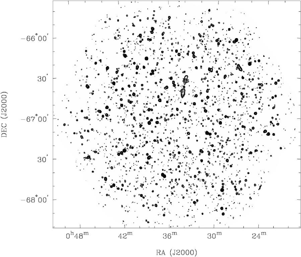
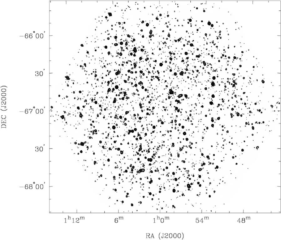
The images corresponding to the 19 pointings constituting each field were lastly combined as a linear mosaic, fully correcting for the primary beam attenuation within the mosaic region but retaining attenuations at the edges of the mosaic to prevent excessive noise amplification there. These mosaic images of the ATLBS regions A & B are shown in Figs. 1 & 2 respectively. The images have an rms noise of Jy beam-1 and the lowest contour level displayed is at . The peak in the image of region A is 104 mJy beam-1 and that in region B is 246 mJy beam-1. The negative peaks in the two images are at levels and Jy beam-1 respectively, which are at the 5–7 level. The ratio of image peak to rms noise exceeds 1000 and the images show no obvious artefacts due to calibration or imaging errors above a level of .
Images in Stokes Q and U were constructed using the same baselines and weighting schemes used in making the Stokes I images. In making these images, we followed the procedure of first constructing wide-field images, isolating the clean components representing emission from the side lobes of the primary beam, subtracted these components from the visibility data, then constructed images representing emission from the main lobes corresponding to each pointing position. The images corresponding to the different pointings were then combined as a linear mosaic to reconstruct the Stokes Q and U emission from ATLBS region A and, separately, region B.
Additionally, we have constructed Stokes V images of the two fields. No obvious sources are seen above the image thermal noise. The peak-to-peak intensity fluctuations in the Stokes V images are in the range mJy beam-1, at ; these values are similar in magnitude to the negative peaks in the Stokes I images indicating that the negative peaks in the Stokes I images are consistent with the image thermal noise.
4.2 A high resolution image of the compact components
As we have noted above, the 750 m array configurations have, additionally, sparse uv-coverage in the 3–5 km range as baselines to the sixth antenna ca06. While we have taken every effort to ensure that the low resolution survey is of the highest quality, we may examine the additional information provided by the baselines to ca06 that could provide some critical information on the compact components in the sources even though the uv-coverage is incomplete. We have used these longer baselines to construct independent images of the two survey regions with higher angular resolution. However, owing to the significant ‘hole’ in the uv-coverage below 3 km in this visibility dataset, the synthesized beam has significant sidelobes and confusion is a serious issue. Therefore, we have aided the deconvolution by using the low-resolution images constructed using the 750-m arrays to identify the sky regions that potentially contain source components.
The first step involved constructing a model representing sources detected outside the primary beam main lobe using all the 750 m array data, including the baselines to the 6-km antenna, and subtracting this from the visibility data. The visibilities were then self-calibrated in phase, using models for source components that were derived by imaging the primary beam main lobe region, and the gains of the data in the two frequency bands were allowed a self-calibration adjustment. The high resolution images were constructed using exclusively the baselines to ca06, which correspond to a uv-coverage that sparsely fills the annulus between 3 and 5 km. Deconvolution of these images was performed iteratively wherein the search region for source components was progressively widened and the component search regions in successive deconvolution iteration steps was derived from deconvolved images of previous steps. In the final deconvolution step the search areas conformed to the regions in the low resolution images—which were constructed using the 750-m baselines—in which the pixel intensity exceeded 0.4 mJy beam-1 (about rms noise).
The high resolution images have been constructed using 5 instantaneous baselines per configuration compared with 10 baselines used to make the low resolution images. The rms noise is, therefore, expected to be about 120 Jy beam-1, and this expectation is very close to that measured in regions of the images that are apparantly source free. Deconvolution iterations were stopped when the peaks in the residual image, within the regions being searched for components, reduced below 0.4 mJy beam-1. This implies that in the high resolution images the fractional flux density exceeding 0.4 mJy are deconvolved and restored with Gaussian components; however, fractional intensities below 0.4 mJy continue to be represented by beams with significant sidelobe structure and their integral flux density over the image will be zero.
The size of the restoring beam following deconvolution was determined by fitting Gaussian models to the main lobes of the synthesized beams. The high resolution images of ATLBS survey regions A and B were made with beam FWHM at P.A. and at P.A. respectively. Since the uv-coverage is an annulus, we might expect that extended source components exceeding the size of these beams would be resolved and their flux densities would be severely attenuated in these images. Nevertheless, source components with size less than these beams would be represented.
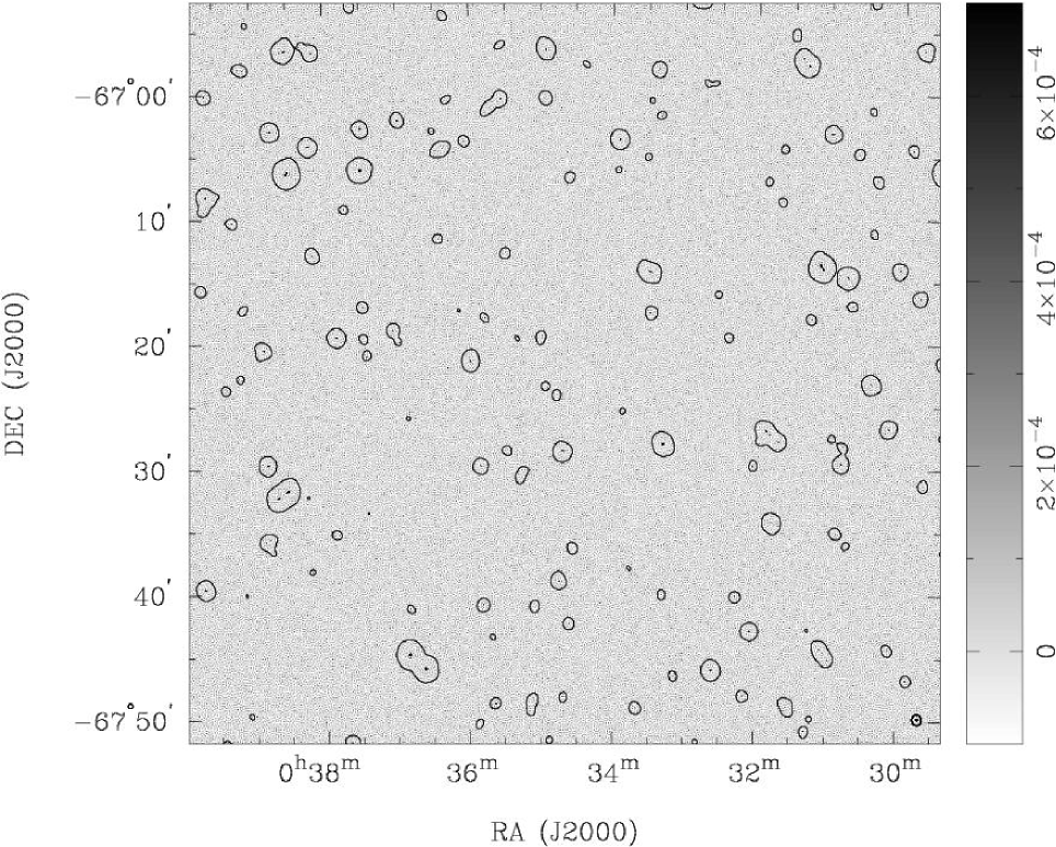
As an example, a portion of survey region A is shown in Fig. 3, where the high resolution image is in grey scales and the corresponding low resolution image is represented using contours. Most of the sources represented by closed contours also have compact components in the grey scale image; sources that appear extended in the low resolution image often appear to have multiple compact components.
5 Properties of the radio sources in the survey
The radio images were scanned, sources identified, and their radio properties listed by an automated algorithm. The routine IMSAD in MIRIAD was modified for this purpose. Only the sky region where the primary beam response in the mosaic exceeds 50% was searched for sources, and flux density estimates were corrected for the primary beam attenuation.
Islands in the low resolution images, with connected pixels exceeding 0.4 mJy beam-1, were considered to be independent sources. Thus, the ATLBS source catalogue presented herein includes all sources that have a peak flux density exceeding 0.4 mJy beam-1 in the low resolution images. The centroid position of these connected pixels was listed as the source position and the source name was derived from this centroid position. Sources were automatically classified as unresolved, extended Gaussian or composite based on their structure in the low resolution image and the success in modeling the images using single-component Gaussians. Peak and total flux densities were estimated for each source, both in the low resolution image and separately in the high resolution image. Extended sources without composite structure were fitted using single Gaussian models and the fit parameters as well as deconvolved source sizes were derived.
The fractional integrated polarized intensity was estimated for the ATLBS sources from the low resolution images in Stokes Q, U and I. Image pixels in which the Stokes I intensity exceeded 0.4 mJy beam-1 were considered, pixel intensities in Stokes Q, U and I were summed separately, a measure of the integrated polarized intensity was estimated by computing , where and represent the pixel-summed image values in Stokes Q and U respectively, the integrated polarized intensity was set to zero if the signal-to-noise ratio in this estimate was less than unity, the polarized intensity estimate was debiased (as described below) and the fractional integrated polarized intensity was computed as the ratio of integrated polarized intensity to integrated total intensity.
The measured integrated polarized intensity was debiased with a simple first-order correction to derive an estimate , where is the standard deviation of the errors in Stokes Q and U image pixels and represents the fractional increase in noise variance in the pixel-summed values. To estimate the fractional increase , we assumed (i) a Gaussian profile for the beam and, therefore, a Gaussian power spectrum for the noise variance, and (ii) a ‘top-hat’ function for the integration area and, therefore, a form for the noise filter function corresponding to the pixel summation; is the Bessel function of the first kind. The pixel averaging in the image domain is, in effect, a convolution in the image domain that corresponds to a multiplication of the power spectrum in the transform domain by a form window. Consequently, the noise in the pixel-summed values would have a variance that is the integral of this windowed power spectrum. The noise variance in the pixel summed values is a factor greater than the noise variance in the individual image pixels, and is proportional to
| (1) |
where is the summation area (in units of radians2) and is the FWHM of the beam (in units of radians). The fractional increase versus the number of pixels in the summation is shown in Fig. 4. The ATLBS images have 1.75-arcsec pixels and, as expected, the variance in the pixel summation rises as the square of the number of pixels in the regime where the summation is over an area less than the beam area, where as the variance in the pixel summation rises proportional to the number of pixels in the regime where the summation area exceeds the beam area. The break at about where the summation is over a beam area is because the noise in image pixels is correlated within beam areas and uncorrelated on larger scales.

In the case of extended sources the polarization position angle may vary over the source; therefore, the integration of Stokes Q and U values over sources, which correspond to measurements of Stokes parameters using beams in which the sources are unresolved, may result in low fractional polarization. The fractional integrated polarized intensities estimated above treat all sources over the entire range of flux densities as unresolved and these values may be a useful comparison of fractional integrated polarizations versus flux density.
In the case of the imaging using the 750-m array data, the synthesized beam has small amplitude sidelobes because the uv-coverage is almost complete. However, in the case of the high resolution imaging the synthesized beam is very different from a Gaussian approximation to the main lobe; therefore, estimating integral flux densities of sources in the high resolution image suffers uncertainties and requires careful understanding of the inherent limitations arising from the annular visibility coverage and the cutoff level adopted during deconvolution.
Within the search region, the farthest distance of a source from pointing centres is . Therefore, owing to the finite bandwidth of the frequency channels in the multi-frequency continuum data, visibility amplitudes at the longest baseline of 5020 m would be expected to have a worst case attenuation to 0.45 of the true value. Simulations using the visibility coverage used to construct the high resolution images and taking into consideration the channel bandwidth corresponding to the observations suggest a worst case attenuation of source peaks to 0.8 of their true value in the high resolution images. We have modeled the bandwidth-related attenuation using a functional form fitted to the simulation results and used this to scale the peaks derived from the high resolution images.
In the high-resolution image, the search for the peak flux density is over a ‘footprint’ on the sky corresponding to the area enclosed by the contour at 0.4 mJy beam-1 in the low-resolution image, or the contour at half the peak flux density if this is lower. The median size of the footprint, for sources with total flux density exceeding 0.4 mJy is 107 beam areas (of the high-resolution image). Our algorithm estimates peak flux densities in the high resolution images by searching for the peak within the corresponding footprint. The probability of a spurious peak of flux density 0.4 mJy occuring in the high resolution images and within the footprint area is below 5%; therefore we may consider those tabulated peaks exceeding 0.4 mJy beam-1 as reliable at the 95% confidence level.
The integrated flux density of the sources in the high resolution image were estimated by summing the flux densities in the compact components. An iterative algorithm was adopted wherein the peak within the ‘footprint’ was located, a Gaussian fit made to the component corresponding to the peak and the Gaussian component subtracted from the high resolution image. Successive peaks—including positive and negative peaks—were located, fitted with Gaussian components and subtracted until the absolute value of the peak residual was below a threshold of 0.5 mJy beam-1. Thus, the listed values of integrated flux densities in the high resolution images is an estimate of the total flux density in compact components exceeding 0.5 mJy; in case the peak within the source ’footprint’ is less than 0.5 mJy then the listed integrated flux density is simply the peak flux density.
A total of 511 sources were identified in Field A and 585 sources in Field B. The two fields have a slight overlap in which there are two common sources; therefore, the number of sources in our catalogue exceeding 0.4 mJy beam-1 peak flux density is 1094 over the 8.42 deg2 sky area.
Of the 484 sources with total flux density in the range 0.4–1.0 mJy, 409 were classified as unresolved in the low resolution images made with beam FWHM of . Of the 75 extended sources (15% of the sources in the 0.4–1.0 mJy range), 64 were deemed to be representable using a single Gaussian model; only 11 sources were classified as composite. The fraction of sources classified to be extended increases to 28% in sources with flux density in the range 1–10 mJy and about half of these sources are deemed composite in structure. As much as 70% of sources in the 10-100 mJy range in flux density are extended, with three-fourths of these classified as composite. The fraction of sources that are deemed extended and with structure well fit by single Gaussian models is about 15% over the entire flux density range 0.4–100 mJy; however, the fraction that is deemed as possessing composite structure increases with flux density rising from about 2% for the sub-mJy population to above 50% for sources with 100 mJy flux density.
The angular size for the ATLBS sources were estimated by measuring the area enclosed by the contour at 0.4 mJy beam-1, assuming that the source has a Gaussian profile, and computing the source width at half maximum. This estimate is expected to be conservative, and yields median angular size of for sources with flux density below 10 mJy, rising to for sources in the 10-100 mJy bin. As compared to the linear size distribution derived by Windhorst et al. (1990), the median angular size of the ATLBS sources appears substantially larger and the distribution in angular size appears to cutoff more sharply. Most ATLBS sources appear only marginally resolved in the low-surface-brightness images made with beam FWHM of about , and we postpone a discussion of the angular size distribution of the ATLBS sources to later papers where detailed structural information is presented.
A listing of the ATLBS radio sources is in Table 2, where we list the source names and centroid positions, classification type using codes ‘P’ for unresolved sources, ‘G’ for resolved sources that may be well fit with single Gaussians and ‘C’ for sources with composite structure. Total and peak flux densities derived from the ATLBS survey images of beam as well as those derived from the high resolution images are listed. Percentage integrated polarization is in the last column of the Table.
The absolute flux density scale is based on the adopted flux density of the primary calibrator PKS B1934638, which is within 2% of the Baars et al. (1977) scale. The absolute position of the phase calibrator has been measured with respect to the International Celestial Reference Frame (ICRF) using long baseline interferometers (Ma et al., 1998). The calibrated visibilities are expected to have 8% amplitude errors because of discrete source confusion within the primary beam during the calibrator observations. As a consequence, the initial model images, which serve as an input to the self-calibration and also determine the absolute astrometry might have a systematic position error of . Image noise contributes an rms error of (2/SmJy) arcsec in positions of sources, which adds in quadrature to the systematic error term (SmJy is the source flux density in mJy). At the flux limit of 0.4 mJy, the position error may be as large as or a tenth of the synthesized beam FWHM. The image dynamic range is 1000, which implies that subsequent to self-calibration we may have residual antenna based phase calibration errors of rms or, equivalently, 1.4% amplitude errors in the calibrated visibilities used in the image making. The errors in peak and total flux density estimates are dominated by the image noise for sources below about 4 mJy, and may be as much as 20% for the faintest sub-mJy sources detected in the survey. The listed total and peak flux densities were estimated from the ATLBS low-resolution survey images and the corresponding high resolution images; these images have rms noise of 0.085 and 0.12 mJy beam-1 respectively.
| Source name | RA | DEC | Type222Source types: P denotes an unresolved object, G denotes a single Gaussian component, C denotes a composite source. and are the total flux density and peak flux density of the source as measured using the ATLBS low resolution images with beam. and are, respectively, the integrated flux density of compact components in the source and the peak flux density as measured using the high resolution image of the source made with beam. The last column lists , which is the percentage integrated polarization in the source. | % Pol. | ||||
| (J2000.0 epoch) | (mJy) | (mJy) | (mJy) | (mJy) | ||||
| J0038.96806 | 00:38:57.60 | 68:06:03.6 | G | 1.45 | 0.96 | 0.79 | 0.79 | 20.2 |
| J0032.66805 | 00:32:39.62 | 68:05:23.7 | G | 20.35 | 19.93 | 8.09 | 5.75 | 0 |
| J0035.76805 | 00:35:46.93 | 68:05:45.8 | P | 0.87 | 1.05 | 0.97 | 0.97 | 37.3 |
| J0032.26804 | 00:32:17.02 | 68:04:00.0 | P | 3.96 | 3.98 | 3.35 | 3.28 | 0 |
| J0033.06803 | 00:33:01.15 | 68:03:33.1 | P | 0.97 | 0.86 | 0.95 | 0.95 | 0 |
| J0039.46801 | 00:39:24.57 | 68:01:34.9 | P | 1.85 | 1.55 | 1.06 | 1.02 | 9.9 |
| J0034.16801 | 00:34:07.57 | 68:01:45.4 | P | 1.97 | 1.95 | 1.06 | 1 | 6.9 |
| J0039.66800 | 00:39:41.03 | 68:00:04.5 | P | 13.28 | 13.42 | 13.21 | 6.5 | 1.9 |
| J0039.16800 | 00:39:10.50 | 68:00:35.4 | P | 0.59 | 0.61 | 0.57 | 0.57 | 0 |
| J0040.66800 | 00:40:36.30 | 68:00:13.8 | G | 0.89 | 0.6 | 0.5 | 0.5 | 2.8 |
| J0037.56800 | 00:37:32.00 | 68:00:24.5 | P | 0.88 | 1.05 | 1.09 | 1.07 | 17.6 |
| J0029.46759 | 00:29:25.83 | 67:59:54.1 | P | 1.46 | 1.5 | 1.36 | 1.34 | 7.8 |
| J0036.26800 | 00:36:15.60 | 68:00:18.5 | P | 0.78 | 0.87 | 1.14 | 0.96 | 0 |
| J0039.96759 | 00:39:57.84 | 67:59:23.8 | P | 0.73 | 0.5 | 0.47 | 0.47 | 37.6 |
| J0035.56758 | 00:35:35.71 | 67:58:48.7 | P | 1.7 | 1.64 | 1.93 | 1.68 | 0 |
| J0028.86758 | 00:28:51.34 | 67:58:28.3 | P | 1.16 | 0.68 | 0.69 | 0.69 | 14.5 |
| J0030.86758 | 00:30:49.93 | 67:58:11.2 | G | 1.11 | 0.95 | 1.11 | 0.91 | 9.2 |
| J0032.66757 | 00:32:39.23 | 67:57:59.5 | G | 1.04 | 0.85 | 0.65 | 0.65 | 23.6 |
| J0038.16757 | 00:38:09.76 | 67:57:09.2 | P | 1.39 | 1.32 | 1.37 | 1.19 | 0 |
| J0029.06755 | 00:29:00.17 | 67:55:50.2 | P | 124.65 | 123.4 | 127.58 | 90.22 | 2.9 |
| J0033.66756 | 00:33:39.33 | 67:56:37.0 | P | 1.75 | 1.68 | 0.55 | 0.55 | 17.6 |
| J0041.76756 | 00:41:45.48 | 67:56:00.9 | P | 0.79 | 0.76 | 0.81 | 0.81 | 58.7 |
| J0027.26755 | 00:27:13.05 | 67:55:01.3 | P | 5.4 | 5.32 | 1.98 | 1.74 | 5.2 |
| J0042.26755 | 00:42:16.02 | 67:55:10.0 | P | 1.97 | 1.83 | 1.2 | 1.03 | 10.6 |
| J0040.46755 | 00:40:24.63 | 67:55:12.2 | P | 0.99 | 0.88 | 0.8 | 0.71 | 4.2 |
| J0042.76754 | 00:42:43.52 | 67:54:26.2 | G | 5.36 | 4.26 | 5.4 | 3.63 | 0 |
| J0035.66754 | 00:35:39.81 | 67:54:48.0 | P | 0.77 | 0.63 | 0.63 | 0.53 | 12 |
| J0035.46754 | 00:35:24.59 | 67:54:11.8 | P | 1.11 | 0.96 | 0.4 | 0.4 | 11.5 |
| J0028.96753 | 00:28:55.76 | 67:53:34.6 | G | 1.59 | 1.42 | 0.51 | 0.51 | 8.6 |
| J0027.36753 | 00:27:18.51 | 67:53:10.4 | P | 4.41 | 4.75 | 1.78 | 1.41 | 4 |
| J0034.26753 | 00:34:12.81 | 67:53:22.9 | C | 2.44 | 1.66 | 0.63 | 0.54 | 5.4 |
| J0030.26753 | 00:30:15.01 | 67:53:27.1 | P | 2.53 | 2.65 | 2.87 | 2.26 | 0 |
| J0039.56753 | 00:39:34.19 | 67:53:37.6 | P | 0.62 | 0.57 | 0.45 | 0.45 | 0 |
| J0032.36753 | 00:32:20.55 | 67:53:35.9 | P | 0.84 | 0.97 | 1.26 | 1.09 | 28.7 |
| J0036.06753 | 00:36:00.14 | 67:53:25.2 | P | 0.41 | 0.51 | 0.51 | 0.51 | 58.4 |
| J0042.16752 | 00:42:08.14 | 67:52:07.5 | P | 4.44 | 4.3 | 3.13 | 1.75 | 0 |
| J0033.16753 | 00:33:09.17 | 67:53:26.1 | P | 0.41 | 0.44 | 0.4 | 0.4 | 32 |
| J0039.66752 | 00:39:40.53 | 67:52:40.2 | G | 1.68 | 0.72 | 0.83 | 0.68 | 19 |
| J0039.46752 | 00:39:26.68 | 67:52:12.2 | P | 1.25 | 1.28 | 1.51 | 1.29 | 15.1 |
| J0028.96751 | 00:28:54.12 | 67:51:27.5 | G | 2.65 | 2.29 | 0.46 | 0.46 | 4.6 |
| J0033.36752 | 00:33:22.12 | 67:52:19.1 | P | 0.46 | 0.58 | 0.45 | 0.45 | 21.5 |
| J0037.66751 | 00:37:39.87 | 67:51:50.5 | P | 1.57 | 1.61 | 1.54 | 1.04 | 7.7 |
| J0041.26751 | 00:41:12.15 | 67:51:23.6 | P | 0.66 | 0.55 | 0.48 | 0.48 | 0 |
| J0032.86751 | 00:32:49.14 | 67:51:51.0 | P | 0.54 | 0.49 | 0.48 | 0.48 | 23 |
5.1 Completeness and reliability of the survey
Reliability of source detection is a major issue in most surveys, particularly interferometer surveys that have poor visibility coverage. The ATLBS survey is unique in that the entire survey regions are observed with complete visibility coverage! Therefore, the synthesized beams are well behaved and the reliability of the survey is determined by the image thermal noise. The noise in the ATLBS images are well defined from the data using Stokes V images: the rms noise is 85 Jy beam-1. We have limited the catalogue to sources detected with a peak flux density exceeding 0.4 mJy beam-1, which is 4.7 times the rms noise. At this level, the Stokes V images have 4 peaks exceeding 0.4 mJy beam-1 over the entire survey area and these are in the range 0.4–0.5 mJy beam-1, indicating that about 0.4% of the sources in the catalogue might be spurious noise peaks and that these spurious sources would be close to the flux limit of the catalogue.
In any survey image, the observed flux density of a source would be the true flux density plus thermal noise. Depending on the value of the noise at the position of the source, the estimated flux density would be altered. When sources are binned in flux density, noise results in movement of sources up or down bins. In effect, the source counts are smoothed by a function whose width depends on the thermal noise in the image. In the mJy and sub-mJy regime that is being explored in the ATLBS survey, the differential source counts steeply decrease with increasing flux density and, therefore, we expect that a net excess of faint sources would be detected because some sources below the flux density cutoff would be noise biased to lie above the detection threshold.
To estimate the completeness and reliability of the ATLBS survey and assess the effect of noise bias on the detection of sources, we have made simulations in which sources were assumed to have a distribution in flux density corresponding to the counts derived by Hopkins et al. (2003). Owing to the image rms noise of 85 Jy beam-1, the expectation from the simulations is that the number of sources detected in the 0.4–0.8 mJy bin would be enhanced by 16%, that in the 0.8–1.6 mJy bin would be enhanced by 2.5% and that in octave bins at higher flux density would be altered by less than a percent. As expected, the effect is greatest close to the flux density cutoff. 18% of the sources in the 0.4-0.8 mJy bin are translated to adjacent bins—13% to below 0.4 mJy and 5% to above 0.8 mJy—but this is overcompensated by sources that are noise biased and translated up in flux density from below the cutoff.
To summarize, spurious sources are extremely rare and constitute only about 0.4% of the sources detected above the cutoff; 13% of sources with true flux density in an octave bin above the cutoff would be noise biased to values below the cutoff and, therefore, would fail to enter the catalogue; however, as much as 27% of the sources detected in the lowest octave bin of 0.4-0.8 mJy are expected to be genuine sources with true flux density below the cutoff that are noise biased to lie above the detection threshold and, therefore, enter the catalogue.
5.2 Confusion and source blending in the survey
A limitation to the reliable detection of discrete radio sources in radio surveys is confusion, which is because the radio image is a convolution of the true sky with the telescope beam. In surveys that are made using interferometer arrays and with sparse visibility coverage, the synthesized beams have significant sidelobes. Along with the limitations to the dynamic range arising from calibration errors, this makes it difficult to distinguish all of the radio sources in the survey area although they may be above the detection threshold as defined by the image thermal noise. The confusion limit on source detection is related to the filling factor in the visibility plane.
The identification of discrete sources in the ATLBS survey was made using the low resolution images, which were made with complete visibility coverage and, therefore, with well defined synthesized beams. The source catalogue that is the basis of the study of the radio source population was also derived from this low resolution image. Therefore, classical confusion and its effects on source selection and completeness and reliability are simply related to the finite resolution of these ATLBS survey images. A measure of the degree to which confusion and source blending result in errors in source counts is how sparsely sources are observed to cover the sky, which depends on the number of beam areas that are observed to be occupied by sources. In the ATLBS low resolution images, the number of effective beam areas per source detected is about 50.
Because of the low angular resolution in the ATLBS survey, confusion manifests in blending of discrete radio sources. We have estimated the ‘blending correction’ from simulations. Sources were assumed to span a range 0.1–409.6 mJy in flux density and Poisson random distributed over the sky area. A distribution in flux density corresponding to the source counts derived by Hopkins et al. (2003) was adopted, which was based on the Phoenix deep survey (PDS). Sources were deemed to be confused if they were connected by a contour at a level of 0.4 mJy beam-1, which was the criterion adopted while forming the ATLBS source catalogue. Confusion between sources in different flux density bins, as well as blending of multiple sources, was allowed for in the simulations. The high surface density of sources with low flux density and the large sky areas covered by the point spread functions associated with sources with relatively higher flux density together result in a confusion between weak sources with the stronger sources. The simulations revealed that for the adopted PDS source counts and the image point spread function corresponding to the ATLBS, confusion results in a significant reduction in the number of sources in octave-band flux-density bins below about 1 mJy, and a small fractional increment in source counts at higher flux densities. Based on the simulations, we estimate that the blending correction factor, owing to classical confusion, is as much as 1.2 in a 0.4–0.8 mJy bin, about 1.02 in a 0.8–1.6 mJy bin, and less than 2% in higher flux density bins.
The high resolution images were constructed from sparse visibility coverage and, consequently, confusion is indeed an issue that limits the elucidation of the high-resolution structures. Only 1% of the visibility plane is covered by the data used to reconstruct these images. As discussed above, the high-resolution images were examined only in the regions where sources were identified in the low resolution images. Operationally, we have used the low resolution images to define the source regions as a constraint during the deconvolution of the high resolution images. This restricted the sources in the high resolution image to be within 2% of the total survey area and resolves the ambiguities arising from the poor visibility coverage and consequent confusion in the high resolution imaging. We estimate that even if every one of the discrete sources identified in the ATLBS survey were a triple, the number of beam areas per source component would be 20 in the case of the high resolution image. Moreover, in this manuscript we restrict to using only estimates of the peak and integrated flux densities of the high resolution images to derive indicators for the source complexity and diffuseness. Detailed high-resolution radio structures of the ATLBS sources, based on followup observations that provide improved visibility coverage, will be presented in later ATLBS related publications.
5.3 The source counts
The number density of ATLBS sources detected with peak flux density exceeding 0.4 mJy beam-1 is 130 sources per square degree.
The normalized differential source counts derived from the source list are shown in Fig. 5. The total flux densities were binned in octave bin ranges: 0.4–0.8, 0.8–1.6, 1.6–3.2 and so on till 204.8–409.6 mJy. We plot the normalized differential source counts versus the mean flux density of sources in the individual bins, the differential counts were normalized to .
The total flux densities of the sources were estimated from the low resolution image: the Gaussian fit parameters were used to infer the total flux densities in the case of unresolved sources as well as those sources with simple structure that were well fit using a single Gaussian model. Composite sources were identified by the significant deviation in the image pixels from the best fit Gaussian model—most of these sources appeared to be composed of multiple components—and in these cases the total flux density was derived by summing the image pixels over the source area. During the synthesis imaging that made the low-resolution image, the iterative deconvolution had been terminated at the 1- noise level and as a result the point spread function for the residual noise slightly differs from the restoring beam used to convolve the CLEAN components: thus the effective beam for weak sources slightly differs from the restoring beam. The algorithm that does the Gaussian fit was limited to using only image pixels exceeding 2- and the fit was weighted by the image pixel intensity to ameliorate the error in the estimation of source flux densities arising from this limitation in image fidelity. Nevertheless, there were a significant number of sources with peak flux density exceeding 0.4 mJy beam-1—30 in all—in which the Gaussian fit parameters were somewhat smaller than the beam size and the estimate of total flux density for these relatively weak sources falls below 0.4 mJy. The source counts in the lowest bin of 0.4–0.8 mJy might be underestimated by 10% due to this effect, and the error bar for this bin has been enhanced to reflect this additional source of uncertainty.

| (mJy) | (mJy) | (Jy1.5 sr-1) | |
|---|---|---|---|
| 0.4–0.8 | 0.59 | 364 | 3.99 () |
| 0.8–1.6 | 1.10 | 289 | 5.74 () |
| 1.6–3.2 | 2.22 | 140 | 7.99 () |
| 3.2–6.4 | 4.63 | 104 | 18.9 () |
| 6.4–12.8 | 8.83 | 70 | 31.2 () |
| 12.8–25.6 | 17.3 | 46 | 55.8 () |
| 25.6–51.2 | 36.3 | 30 | 113.5 () |
| 51.2–102.4 | 76.5 | 11 | 131.6 () |
| 102.4–204.8 | 144.5 | 7 | 207.2 () |
| 204.8–409.6 | 268.4 | 2 | 140.7 () |
The first column lists the bin ranges for the total flux density, the second column lists the mean flux density of the sources in the bins, the third column lists the number of sources detected in each of the flux density ranges and the last column lists the normalized differential source counts corrected for various factors discussed in the text.
The source counts in the flux density bins have been corrected for the primary beam attenuation over the survey area by scaling the count corresponding to each detected source by the ratio of the total area of the survey and the area over which the source is detectable: since we truncate at the level where the primary beam drops to 50%, this correction is relevant only for the lowest octave bin and in this bin the counts were scaled up by a factor 1.33 to account for this effect.
There may be sources with peak flux density below 0.4 mJy beam-1, and missing in the derived source catalogue, which are extended and have total flux density exceeding 0.4 mJy: the derived ATLBS source counts would be an underestimate due to such sources as well. However, analysis of the source structural properties in Sections 5.5 and 5.6 suggests that most sources have simple structures at low flux density levels, at least at the resolution of the ATLBS survey; therefore, we expect any correction owing to extended source structure to be small. If we adopt the model for the angular size distribution of sources derived by Windhorst et al. (1990), which has the median radio source angular size of sources with 1.4 GHz flux density (in mJy) equal to arcsec, and an exponential form for the integral angular size distribution, the resolution corrections required to be made to our derived source counts are less than 1%.
The ATLBS source counts shown in Fig. 5 have been corrected for the primary beam attenuation, noise bias that was discussed in Section 5.1, resolution and blending; these corrected counts are also listed in Table 3. The second column of the Table lists the mean flux density of sources in the bins, column 3 lists the number of sources detected in the individual bins (uncorrected) and the last column lists the derived normalized differential source counts corrected for the effects discussed above.
As a comparison, ATESP survey counts (Prandoni et al., 2001) and the fit to PDS counts (Hopkins et al., 2003) are also shown in Fig. 5. The PDS counts were derived from their survey that covered 4.56 deg2 area and the ATESP survey covered 26 deg2 area; these are comparable to our survey area of 8.4 deg2.
Within the errors, the observed counts appear consistent with the estimates derived by Prandoni et al. (2001) based on the ATESP survey. The counts are, however, systematically lower than that estimated by Hopkins et al. (2003) based on the PDS: in the flux density range 0.8–200 mJy our ATLBS counts are on the average a factor 0.8 of the PDS counts. As was the case for the ATESP survey counts, which do not show an upturn and suggest that any upturn at faint flux density levels is below 1 mJy, the ATLBS counts are also consistent with no upturn down to about 0.6 mJy.
At the faint end of the flux density scale explored by the ATLBS survey, blending reduces the observed counts where as noise bias enhances counts. The blending corrections, as well as our estimates for the enhancement in the observed counts owing to noise bias, might be overestimates because we have assumed the relatively higher counts, based on the PDS survey, for the simulations that estimate these correction factors. Additionally, as discussed above, the counts in the lowest bin might be an underestimate due to missing sources because their peaks may be below the 0.4 mJy beam-1 cutoff or because of image errors arising from the deconvolution algorithm adopted.
A cause for significant discrepancies between different estimates of the source counts at the sub-mJy levels might be field-to-field variations. The relatively large sky area, spread over multiple sky patches, covered by the ATESP survey makes these counts a more reliable indicator of counts at these faint levels and there is good agreement between the ATLBS counts and the ATESP counts in the 0.4–1.6 mJy bins: both are systematically low compared to the PDS survey counts.
The systematic low counts derived from the ATLBS survey is not owing to classical confusion; the ATLBS counts presented here have been corrected for blending confusion. The low counts, relative to the PDS, could be interpreted as arising due to a 30% underestimate in the flux density of sources, or a 20% reduction in numbers of sources. Since the ATLBS has good surface brightness sensitivity, it is expected that the source catalogues derived from the survey would not have any missing flux density. Additionally, the ATLBS survey is potentially capable of detecting extended sources with low surface brightness, which may be missed in other surveys. The low counts are more likely indicating that the ATLBS survey detects a smaller number of sources as compared to surveys like the PDS. It has been pointed out by Hopkins et al. (2003) that the PDS counts are based on a component catalogue, rather than a source catalogue as was the case for the ATESP counts. Source counts derived from such component catalogues would be expected to overestimate the numbers of sources as a result of sources in higher flux density bins degenerating into multiple sources in bins with lower flux densities. The ATLBS survey is a source catalogue owing to the relatively large size of the synthesized beam; therefore, it is unsurprising that the counts derived are consistent with that of the ATESP survey and below the PDS counts.
5.4 The fractional polarization in ATLBS sources
As discussed above in Section 5, we have derived estimates for the percentage integrated polarization for the ATLBS sources using the low resolution images, integrating Stokes Q, U and I over the source, computing the debiased polarised intensity and dividing by the total intensity. The sources were binned in flux density, and the median integrated percentage polarization as well as the mean flux density of the sources in the individual bins were computed; these values are in Table 4. The errors have been estimated using the Efron bootstrap method (Efron, 1979), in which the samples in each bin were randomly resampled with replacement to derive a sampling distribution of the median and, thereby, an estimate of the error in the median. In Fig. 6 we plot the median integrated percentage polarization versus mean flux density for the binned data. The plot clearly shows an increasing fractional polarization with decreasing flux density. This trend is consistent with the observation that among polarized radio sources, the faint sources are more highly polarized than the relatively stronger sources (Taylor et al., 2007).
The binned data were fitted to a power-law to derive the trend:
| (2) |
where is the median percentage integrated polarization and is the mean flux density (in mJy). The fit is also shown in Fig 6. The data appears well fit by this single power-law form over more than a decade in flux density; however, there appears to be a flattening above 10 mJy suggesting that at higher flux densities the fractional integrated polarization in sources may not change with flux density.
| Flux density | Mean flux density | Median integrated |
|---|---|---|
| bin (mJy) | (mJy) | % polarization |
| 0.4–0.8 | ||
| 0.8–1.6 | ||
| 1.6–3.2 | ||
| 3.2–6.4 | ||
| 6.4–12.8 | ||
| 12.8–25.6 | ||
| 25.6–51.2 |
The total flux density of sources has been used in the binning. The quoted errors are 1 standard deviation (1-) values.

We have adopted a signal-to-noise ratio based cutoff that sets to zero estimates of polarized intensity that are below one standard deviation of the expected noise. Such a cutoff may potentially result in a positive residual polarization bias if the polarized intensity has a low signal-to-noise ratio (Leahy & Fernini, 1989). The estimator of fractional integrated polarization, , was separately recomputed assuming a signal-to-noise ratio based cutoff that set to zero estimations that are below two standard deviations of the expected noise: in this case as well the mean percentage polarizations continued to display the trend of increasing fractional polarization with decreasing flux density, although the residual polarization bias in this case is expected to be negative at low signal-to-noise ratios. This test adds weight to our finding that the fractional polarization in radio sources increases with decreasing flux density.
5.5 Complexity of radio sources at sub-mJy flux density

| Flux density | Median flux | Number of | Median |
|---|---|---|---|
| bin (mJy) | density (mJy) | sources | complexity |
| 0.5–0.9 | 0.67 | 339 | |
| 0.9–1.9 | 1.21 | 271 | |
| 1.9–4.7 | 2.72 | 148 | |
| 4.7–16.5 | 7.18 | 143 | |
| 16.5–92.0 | 27.85 | 63 |
The total flux density of sources has been used in the binning. The quoted errors for the median complexity are 1 standard deviation (1-) errors.
The radio sources were identified in the low resolution images as a set of connected pixels with intensity exceeding 0.4 mJy beam-1. These images have a high surface brightness sensitivity and were made with a beam of FWHM about 50. The total flux densities were estimated either from a Gaussian fit to the source image pixels in this low resolution image or, in the case of sources with composite structure, from a summation over the image pixel intensities. Apart from deriving a value for the peak flux density in the low resolution image, we have also separately derived the peak flux densities in each of the sources from the high resolution images, which were made with beam FWHM about .
The ratio of the total flux density, as measured using the low resolution image, to the peak flux density, as measured in the high resolution image, is a measure of the departure of the source appearance from that of an unresolved object of size well below . This ratio , which we adopt as a measure of how complex sources appear to be, is a measure of how complex the source structure is when observed with a beam of FWHM . is expected to be unity for unresolved sources, and exceed unity for resolved sources. will exceed unity not only in the case of sources with extended emission that is resolved by a beam, but also in the case where the source is composed of multiple components (which may be individually unresolved). Additionally, will exceed unity in cases where the source in the low resolution image is confused, for example, because two or more unresolved and unrelated sources lie close together on the sky and within the beam of the low resolution image. As discussed in Section 5.2, such blending is not expected to be an issue at flux density exceeding 0.8 mJy, and the effect of blending on source counts at these higher flux density levels is expected to be less than 2%.
There are 1063 sources in the ATLBS survey with total flux density exceeding 0.4 mJy. The median for these sources is 1.28. 20% of the sources have exceeding 2.0, which implies that when observed with beam FWHM , close to a fifth of the ATLBS sources are either doubles, triples or more complex sources or have more than half of their total flux density in extended emission components.
In Table 5 we list the median complexity of sources in bins of total flux density. In Fig. 7 is shown the distribution of median complexity versus total flux density. The errors listed in the table, as well as the error bars in the figure, correspond to 1 standard deviation errors that were estimated from the data using the Efron bootstrap method (Efron, 1979). The bins were chosen to have widths increasing with flux density; bin widths are proportional to (flux density)3/2. Fig. 7 shows that the source complexity increases with increasing total flux density. This is consistent with earlier findings that the median angular size of sources declines towards lower flux density, and that fainter radio sources are increasingly compact.
The derived source complexity has errors owing to the error in the estimates for source total flux density and the peak flux density in the high-resolution image. Values of total flux density have rms errors less than 20%; errors are less than 10% in sources with flux density exceeding 1 mJy. The peak flux density in the high resolution image has an absolute rms error of 0.12 mJy. As discussed above in Section 5, the median source ‘footprint’, which is the search area for the peak in the high resolution image, has 107 (high resolution image) beam areas. It follows that the probability of a chance peak within the ‘footprint’ exceeding 0.45 mJy is less than about 1%. Spurious noise peaks within the footprint, which exceed the true peak flux density of the source, would result in an over estimate of the peak flux density and lead to an underestimate for the source complexity. The estimate for source complexity would, therefore, be a lower limit to its true value and this underestimation would be greater in sources with smaller flux density.
If we consider sources in the 0.5–0.9 mJy bin, which has the sources with lowest flux density, the median flux density is 0.67 mJy and the sources are estimated to have a median complexity of . For sources in this bin, the probability that a noise peak within the source footprint exceeds 0.45 mJy and, consequently, the complexity is underestimated to have a value below 1.19 is less than 1%. Therefore, it is unlikely that image noise causes the median complexity of sources in the 0.5-0.9 mJy bin to be as low as 1.19. The effects of image noise are less significant in the source complexity estimates at higher flux densities. The low value for the source complexity estimated for the sub-mJy ATLBS population, and the rise in complexity with flux density, are likely to be genuine.
If we consider sub-mJy sources in the flux density range 0.7–1.0 mJy, for which the flux densities all exceed six times the rms noise in the high resolution image, a significant number of these sources may have complexity exceeding 2.0 despite the noise. Even if all of these sources have true exceeding 2.0, only in about a sixth of these sources do we expect the noise peaks in the high resolution image to result in estimates for the complexities below 2.0. We find that only 8% of sources in this flux density range have complexity exceeding 2.0. In contrast, 28% sources in the flux density range 1–10 mJy have complexity exceeding 2.0, and 55% sources in the 10-100 mJy range have complexity exceeding 2.0.
5.6 Diffuse emission associated with sub-mJy radio sources
The parameter introduced above is a measure of the degree of source complexity, but does not distinguish sources with extended or diffuse emission from sources with multiple components, composite structure composed of compact components, and confusion.

| Flux density | Number of sources | Median diffuseness |
|---|---|---|
| (mJy) | ||
| 0.5–0.9 | 339 | |
| 0.9–1.9 | 271 | |
| 1.9–4.7 | 148 | |
| 4.7–16.5 | 143 | |
| 16.5–92.0 | 63 |
The total flux density of sources has been used in the binning. The quoted errors for the median diffuseness are 1 standard deviation (1-) errors.
The high resolution images described in Section 4 were constructed using a visibility coverage that is an annulus and the beam FWHM is about ; therefore, it is expected that extended emission on scales exceeding would be resolved out and absent in these images. The fractional flux density in extended emission, which would be missing in the resolution images, may be characterized by the ratio of the total flux density in the low resolution images to the integrated flux density in the high resolution images. We refer to this ratio parameter as , representing the degree of diffuse emission in the source or, in other words, a diffuseness parameter. This parameter is expected to reveal the quantum of flux density in extended diffuse emission.
The median value of for the sources with total flux density exceeding 0.4 mJy in the ATLBS survey is ; about half of the sources have more than a tenth of their flux density in diffuse emission. The median is significantly smaller than the median , which is 1.28, as might be expected since the complex structure is only partly diffuse structure. About 10% of the ATLBS sources with flux density exceeding 0.4 mJy beam-1 have exceeding 2.0; these sources have over half of their total flux density in diffuse emission.
We have computed the median value of the degree of diffuse structure—median —in bins of total flux density, where the source total flux density is determined from the low resolution images with high surface brightness sensitivity. In Fig. 8 is shown the variation in with total flux density; the values are in Table 6. The errors were estimated from the data, as above, using the Efron bootstrap method. The ATLBS radio source population does not show any significant trend in the degree of diffuse emission versus total flux density, although the source complexity shows a significant rise towards higher total flux density. The increased complexity in sources with higher flux density appears to be owing to the sources being composed of multiple compact components rather than increased fraction of diffuse emission. The fractional flux in diffuse emission appears to be fairly constant, independent of total flux density, at least in the range 0.4–100 mJy.
The total flux density is determined from the low resolution images with rms noise 0.085 mJy beam-1. The fractional error in this estimate is at most 20%, and less than 10% for sources with total flux density exceeding 1 mJy. The integrated flux density estimate derived from the high-resolution image is a summation of the flux densities in compact components with peak exceeding 0.5 mJy; in those cases where no compact component exceeds this threshold the estimate for integrated flux density is simply the value of the peak within the ‘footprint’. Therefore, the tabulated values of integrated flux density of compact components, which are used in estimating , represent a lower limit to the integrated flux in compact components and may miss compact components that have peak flux density below 0.5 mJy beam-1 in the high resolution image. On the other hand, the high resolution images have an rms noise of 0.12 mJy beam-1 and in cases where the source does not have compact components above this noise the noise peak within the ‘footprint’ would be tabulated as the integrated flux density of compact components. There is less than 1% chance of a noise peak exceeding 0.45 mJy within the footprint; however, peaks exceeding 0.35 mJy are expected with 25% probability. Weak compact components that are missed result in an overestimate in , noise in the high resolution image results in underestimates for . Owing to the image rms noise, sources with a given total flux density are unlikely to have exceeding an upper bound; for example, it is unlikely that sources with total flux density below 0.56 mJy have .
We define the sky area of any source to be the area enclosed by the 0.4 mJy beam-1 contour in the low resolution image of the source. We have estimated the integrated flux density in the compact components in any source by summing the flux densities of all the components in the high resolution image that are located within the sky area of the source. This integrated flux density exceeds the peak flux density of the source (as measured in the high resolution image) in most cases, as expected. The excess may be quantified as the ratio of the integrated to the peak flux density; both measured in the high resolution images. We find that this excess increases with increasing flux density. 36% of sources with flux density exceeding 10 mJy have this ratio of the integrated to peak flux density exceeding 2 and 10% of sources in the 1–10 mJy range have integrated flux density exceeding the peak by a factor 2 or more. In the sub-mJy population of sources that have an integrated flux density in the 0.4–1.0 mJy range (484 sources), where estimates of this ratio may be considered to be lower limits, less than 1% of sources have listed integrated flux density exceeding the peak by a factor of 2. This finding is consistent with a change in the radio structure of ATLBS sources with flux density in which the abundance of multiple compact components is greater in sources with higher flux density: the fainter sources may be dominated by sources with a single compact component whereas brighter sources have double and triple compact structures.
6 Summary
We have used the Australia Telescope Compact Array to survey 8.42 deg2 sky area at a radio frequency of 1388 MHz. The interferometer observations were made in a mode designed to mosaic image the wide field with complete visibility coverage, and hence low confusion, and with exceptional surface brightness sensitivity. The data were used to reconstruct (a) a low resolution image, with beam FWHM and rms noise 0.08 mJy beam-1, and (b) a high resolution image with beam FWHM of . Whereas the low resolution image reproduces the extended and diffuse radio emission associated with sources in the fields, the high resoluion image resolves out structure on scales exceeding the beam size. Together, the images provide an estimate of the structural properties of the mJy and sub-mJy radio sources. We refer to our radio survey as the Australia Telescope low brightness survey, and use the acronym ATLBS.
A total of 1094 radio sources with peak flux density exceeding 0.4 mJy beam-1 in the low resolution image were cataloged and their source properties estimated. The source detections correspond to a density of 130 sources per square degree. The studies presented herein have considered only sources with peak flux density exceeding about 5 times the rms noise in the image.
The normalized differential source counts derived from the ATLBS shows no evidence for an upturn down to about 0.6 mJy; the ATLBS counts are consistent with the ATESP source counts, but relatively low compared to many other surveys, including the PDS. This result suggests that there is no substantial population of low surface brightness sources or source components at these flux densities that have been missed by previous surveys. The ATLBS counts—as also ATESP counts—are relatively low compared to many other counts perhaps because our counts are based on a source catalog, rather than a component catalog. As far as we know, blending has been considered and corrected for the first time in the work presented herein; blending is of concern in surveys such as the ATLBS that aim to go deep in surface brightness sensitivity. The derived ATLBS source counts have been corrected for blending, noise bias, resolution and primary beam attenuation over the survey area.
The derived source counts are consistent with that of the ATESP survey suggesting that the relatively large sky coverage of these surveys is key to robust measurement of source counts. The considerable scatter in the derived differential source counts at about 1 mJy flux density between the various surveys that were made with relatively smaller sky coverage is perhaps owing to genuine field-to-field variations in counts. To summarize, the work presented here emphasises the importance of constucting source catalogs, accounting for blending and noise bias, and making large area surveys in order to refine our understanding of differential source counts at sub-mJy and mJy flux densities.
The main results presented in this paper concern the statistical properties of the radio structure and polarization in sub-mJy sources compared to the mJy radio source population. We have defined a complexity parameter as the ratio of the total flux density of the source to the peak flux density in the high resolution image, this parameter is a measure of the source complexity and the departure of the source structure from an unresolved single compact component. Additionally, we have defined a diffuseness parameter as the ratio of total flux density to the sum of the flux density in compact components, this parameter is a measure of the flux density in diffuse emission components. These measures of morphology have been computed for all ATLBS sources. The points arising from an examination of the sources above and below 1 mJy flux density are listed below.
-
1.
In the low-resolution images made with beam, the fraction of extended sources rises from 15% for the sub-mJy population to 28% for 1–10 mJy sources and to 70% for 10–100 mJy sources. At this resolution, only 2% of sub-mJy sources are observed to have composite structure where as this fraction rises to 15% for 1–10 mJy sources and 50% for 10–100 mJy sources.
-
2.
Less than 1% of the sub-mJy ATLBS sources have been observed to have multiple compact components. However, about 10% of 1–10 mJy sources have multiple compact components and this fraction rises to 36% in sources in the 10–100 mJy range.
-
3.
The median complexity for ATLBS sources is 1.28 and the median diffuseness is 1.09. 20% of ATLBS sources have exceeding 2.0, implying that a fifth of the sources are doubles or triples or have more than half their flux density in extended emission. 10% of the ATLBS sources have exceeding 2.0, implying that a tenth of the sources have more than half their flux density in diffuse emission.
-
4.
We observe no significant trend in median with flux density. However, rises significantly with increasing flux density. Whereas only 8% sub-mJy ATLBS sources have exceeding 2.0, 28% of 1–10 mJy sources have exceeding 2.0 and this fraction rises to 55% for the 10–100 mJy sources.
The sub-mJy ATLBS sources, with 10% sources having more than half the flux density in extended emission, almost always have a single compact component, if present. On the other hand, sources with higher flux density tend to have a greater fraction of multiple compact components, although the fractional flux density in the diffuse emission might be the same. This is consistent with population synthesis models for the differential source counts wherein the mJy radio source population is dominated by the relatively powerful radio sources, which are often of the hot-spot type with FR-ii structure, and the sub-mJy sources are dominated by the relatively lower power radio sources, which often manifest the FR-i structure with a single compact component.
We have computed the percentage integrated polarized intensity for the ATLBS sources and examined their variation with total flux density. As far as we know, we have formulated herein a polarization bias correction for integrated polarized emission for the first time. We observe an increase in the percentage polarization in the ATLBS sources with decreasing flux density. The median percentage polarization is above 10% in the sub-mJy sources and declines to a few percent in sources with 100 mJy flux density. We have been unable to find any correlation between the percentage polarization and the source properties like size, complexity or the fractional flux in the diffuse emission. Since we do observe a decrease in source complexity in fainter sources, it may be that the increased percentage polarization in the fainter sources is owing to a transition from FR-ii dominated population at higher flux densities to FR-i dominated population. Radio source populations dominated by edge-darkened FR-i jets or relaxed doubles and relict sources with relatively homogeneous magnetic field orientation may suffer less depolarization, due to averaging over the spatial extent of the source, as compared to the FR-ii sources that have more complex spatial structure in their field distributions. Alternately, the increased fractional polarization in the fainter sources may be due to lower internal Faraday depolarization if the fainter sources are at relatively higher redshift and the emission frequency in the rest frame of the source is higher in the case of the fainter sources. Higher resolution radio imaging and redshift measurements of the optical identifications of the ATLBS sources—both of which are currently underway—might shed light on this issue.
The Very Large Array (VLA) survey of the Chandra Deep Field South (Kellermann et al., 2008), together with optical identifications of the radio sources (Mainieri et al., 2008), suggest that the the sub-mJy radio sources above 0.08 mJy are dominated by non-thermal emission associated with early type galaxies hosting AGNs. Padovani et al. (2007) suggest that the dominant population is low-luminosity AGNs of the FR-i type. The ATLBS study of radio source morphology are consistent with this view.
The ATLBS survey has indicated that the sub-mJy radio source population does indeed have a non-negligible fraction of their integrated flux density in diffuse emission. Therefore, it is vital that deep radio surveys be made with adequate surface brightness sensitivity to measure the total radio luminosity associated with the AGNs, and accurately quantify any associated mechanical feedback.
The ATLBS survey regions are being re-observed using extended array configurations of the ATCA to reconstruct source structures with higher angular resolution, to confirm the findings presented in this paper and explore further the radio structural properties of the sub-mJy radio source population. Additionally, the wide fields are being mosaic observed in the optical and IR bands using the CTIO Blanco Telescope and the Anglo-Australian Telescope in a study of the host galaxies and their environments. These observations and the consequent refinements in our understanding of the evolution in extended radio sources will be the subject of forthcoming papers.
Acknowledgments
The ATCA is part of the Australia Telescope, which is funded by the Commonwealth of Australia for operation as a National Facility managed by CSIRO.
References
- Baars et al. (1977) Baars J. W. M., Genzel R., Pauliny-Toth I. I. K., Witzel A., 1977, A&A, 61, 99
- Bock, Large & Sadler (1999) Bock D. C.-J., Large M. I., Sadler E. M., 1999, AJ, 117, 1578
- Efron (1979) Efron, B., 1979, The Annals of Statistics, 7, 1
- Fanaroff & Riley (1974) Fanaroff B. L., Riley J. M., 1974, MNRAS, 164, 31
- Griffith & Wright (1993) Griffith M. R., Wright A. E., 1993, AJ, 105, 1666
- Hopkins et al. (2003) Hopkins A. M., Afonso J., Chan B., Cram L. E., Georgakakis A., Mobasher B., 2003, ApJ, 125, 465
- Jarvis & Rawlings (2004) Jarvis M. J., Rawlings S., 2004, New Astronomy Reviews, 48, 1173
- Kellermann et al. (2008) Kellermann K. I. et al., 2008, ApJS, 179, 71
- Leahy & Fernini (1989) Leahy P., Fernini I., 1989, VLA Scientific Memo No. 161
- Ma et al. (1998) Ma C. et al., 1998, AJ, 116, 516
- Mainieri et al. (2008) Mainieri V. et al., 2008, ApJS, 179, 95
- Padovani et al. (2007) Padovani P., Mainieri V., Tozzi P., Kellermann K. I., Fomalont E. B., Miller N., Shaver P., 2007, to appear in At the edge of the Universe. astro-ph/0701493
- Prandoni et al. (2001) Prandoni I. et al., 2001, A&A, 365, 392
- Sault & Wieringa (1994) Sault R. J., Wieringa M. H., 1994, A&A Suppl Ser., 108, 585
- Subrahmanyan et al. (2007) Subrahmanyan R., Ekers R. E., Saripalli L., Sadler E. M., 2007, in proceedings of “From Planets to Dark Energy: the Modern Radio Universe”, PoS(MRU2007)055
- Taylor et al. (2007) Taylor A. R. et al., 2007, ApJ, 666, 201
- Windhorst et al. (1990) Windhorst R. A., Mathis D. F., Neuschaefer L. W., 1990, in ASP Conf. Ser. Vol. 10, Evolution in the Universe of galaxies, eds. Kron R. G., p.389
- Windhorst et al. (2005) Windhorst R. A., Miley G. K., Owen F. N., Kron R. G., Koo, D. C., 2005, ApJ, 289, 494