Electron heating and acceleration by magnetic reconnection in hot accretion flows

Abstract

Both analytical and numerical works show that magnetic reconnection must occur in hot accretion flows. This process will effectively heat and accelerate electrons. In this paper we use the numerical hybrid simulation of magnetic reconnection plus test-electron method to investigate the electron acceleration and heating due to magnetic reconnection in hot accretion flows. We consider fiducial values of density, temperature, and magnetic parameter $\beta_{e}$ (defined as the ratio of the electron pressure to the magnetic pressure) of the accretion flow as $n_{0}\sim 10^{6}{\rm cm^{-3}}$, $T_{e}^{0}\sim 2\times 10^{9}{\rm K}$, and $\beta_{e}=1$. We find that electrons are heated to a higher temperature $T_{e}=5\times 10^{9}$K, and a fraction $\eta\sim 8\%$ of electrons are accelerated into a broken power-law distribution, $dN(\gamma)\propto\gamma^{-p}$, with $p\approx 1.5$ and $4$ below and above $\sim 1$ MeV, respectively. We also investigate the effect of varying $\beta$ and $n_{0}$. We find that when $\beta_{e}$ is smaller or $n_{0}$ is larger, i.e, the magnetic field is stronger, $T_{e}$, $\eta$, and $p$ all become larger.

1. Introduction

Magnetic reconnection serves as a highly efficient engine which converts magnetic energy into plasma thermal and kinetic energy. The first theoretical model for magnetic reconnection was proposed by Sweet and Parker (Parker, 1958). Ever since then, theoretical studies along this line have been reported in various papers including analytical theories and numerical simulations (Parker, 1963; Drake et al., 2005; Litvinenko, 1996).

Magnetic reconnection has been widely used to explain explosive phenomena in space and laboratory plasmas such as solar flares (Somov & Kosugi, 1997), the heating of solar corona (Cargill & Klimchuk, 1997), and substorms in the Earth’s magnetosphere (Bieber et al., 1982; Baker et al., 2002). Magnetic reconnection also plays an important role in high-energy astrophysical environments such as the magnetized loop of the Galactic center (Heyvaerts et al., 1988), jets in active galactic nuclei (Schopper et al., 1998; Larrabee et al., 2003; Lyutikov, 2003), and $\gamma$ ray bursts (Michel, 1994). For example, by assuming that particle acceleration is due to direct current (DC) electric field and is balanced by synchrotron radiative losses, Lyutikov (2003) found that the maximum energy of electrons is $\sim 100$ TeV. Larrabee calculated the self-consistent current density distribution in the regime of collisionless reconnection at an X-type magnetic neutral point in relativistic electron-positron plasma and studied the acceleration of non-relativistic and relativistic electron populations in three-dimensional tearing configurations.

But so far there is very few work on the magnetic reconnection in hot accretion flows. In accretion flows, the gravitational energy is converted into turbulent and magnetic energy due to the magnetorotational instability (MRI; Balbus & Hawley, 1991). Both analytical works (e.g., Quataert & Gruzinov, 1999; Goodman & Uzdensky, 2008; Uzdensky & Goodman, 2008) and three-dimensional magnetohydrodynamic simulations of black hole accretion flow (Hawley & Balbus, 2002; Machida & Matsumoto, 2003; Hirose et al., 2004) have shown that magnetic reconnection is unavoidable and plays an important role in converting the magnetic energy into the thermal energy of particles. In fact, turbulent dissipation and magnetic reconnection are believed to be the two main mechanisms of heating and accelerating particles in hot accretion flows. In the case of large $\beta$ ($\beta$ is defined as the ratio of the gas pressure to the magnetic pressure), the magnetic reconnection is even likely to the dominant mechanism of electrons heating and acceleration (Quataert & Gruzinov, 1999; Bisnovatyi-Kogan & Lovelace, 1998). On the observational side, flares are often observed in black hole systems. One example is the supermassive black hole in our Galactic center, Sgr A*, where infrared and X-ray flares occur almost every day (e.g., Baganoff et al., 2001; Hornstein et al., 2007; Dodds-Eden et al., 2009). To explain the origin of these flares, we often require that some electrons are transiently accelerated into a relativistic power-law distribution by magnetic reconnection within the accretion flow (e.g., Baganoff et al., 2001; Yuan et al., 2003, 2004; Dodds-Eden et al., 2009; Eckart et al., 2009) or in the corona above the accretion flow (e.g., Yuan et al. 2009), and their synchrotron or synchrotron-inverse-Compton emission will produce the flares.

Regarding the study of the electron acceleration by reconnection, recently many works have been done on the relativistic magnetic reconnection with the approach of Particle-in-Cell (PIC) simulation. Zenitani & Hoshino (2007) presented the development of relativistic magnetic reconnection, whose outflow speed is on the order of the light speed. It was demonstrated that particles were strongly accelerated in and around the reconnection region and that most of the magnetic energy was converted into a “non-thermal” part of plasma kinetic energy. Magnetic reconnection during collisionless, stressed, X-point collapse was studied using kinetic, 2.5D, fully relativistic PIC numerical code in Tsiklauri & Haruki (2007) and they also found high energy electrons. PIC electromagnetic relativistic code was also used in Karlicky (2008) to study the acceleration of electrons and positrons. They considered a model with two current sheets and periodic boundary conditions. The electrons and positrons are very effectively accelerated during the tearing and coalescence processes of the reconnection. All these work investigate the circumstance of the Sun.

In this paper we use the numerical hybrid simulation of magnetic reconnection plus test-electron method to investigate the electron heating and acceleration by magnetic reconnection in hot accretion flows. We would like to note that the results should also be applied to corona of accretion flow and jet, if the properties of the plasma in those cases are similar to what we will investigate in the present paper. Self-consistent electromagnetic fields are obtained from the hybrid code, in which ions are treated as discrete particles and electrons are treated as massless fluid. Thereafter, test electrons are placed into the fields to study their acceleration. The input parameters include density, temperature and magnetic field of the accretion flow. The values of density and temperature of astrophysical accretion flows can differ by several orders of magnitude among various objects. Here we take the accretion flow in Sgr A* as reference (see Yuan et al., 2003, for details), but we also investigate the effect of varying parameters. For the strength of the magnetic field, we consider mainly $\beta_{e}=1$. Here $\beta_{e}$ is defined as the ratio of the electron pressure to magnetic pressure, $\beta_{e}\equiv P_{e}/P_{\rm mag}$. Note that what we usually use in hot accretion flows is the ratio of the gas pressure and the magnetic pressure, $\beta\equiv P_{gas}/P_{\rm mag}$. The hot accretion flow is believed to be two-temperature, with $T_{i}\gg T_{e}$. For a reasonable value of $T_{i}=10T_{e}$ (ref. Yuan et al., 2003), the above $\beta_{e}$ corresponds to the usual $\beta=10$. This is the typical value in the hot accretion flow as shown by MHD numerical simulations (e.g., Hirose et al., 2004). Given that the value of $\beta$ is very inhomogenous in the accretion flow (Hirose et al., 2004), we also consider $\beta_{e}=10,0.1$, and $0.01$.

In Section 2, we use the numerical hybrid simulation of magnetic reconnection to get the structure of self-consistent electric and magnetic fields. In Section 3 we use the obtained electromagnetic fields as the background of test electrons to investigate the electron acceleration. Finally we summarize our results and discuss the application in interpreting the flares in Sgr A* in Section 4.

2. The numerical hybrid simulation of magnetic reconnection

We use the 2.5-D (two-dimensional and three components) hybrid simulation code of Swift (Swift, 1995, 1996) to model the driven steady Petschek mode magnetic reconnection, except that we use a rectangle coordinate system. Quasi charge neutrality is assumed, which can be written as $n_{i}\thickapprox n_{e}=n$.

The momentum equation for each ion as a discrete particle is given by

$$\frac{d\textbf{v}}{dt}=(\textbf{E}+\textbf{v}\times\textbf{B})-\nu(\textbf{u}_{i}-\textbf{u}_{e}),$$ (1)

where v is ion velocity, E is the electric field in units of ion acceleration, B is the magnetic field in units of the ion gyrofrequency, and $\nu$ is the collision frequency. A finite numerical resistivity corresponding to the collision frequency $\nu$ is imposed in the simulation domain (X point) to trigger the reconnection. $\textbf{u}_{e}$ and $\textbf{u}_{i}$ are the bulk flow velocities of electrons and ions. In particular, $\textbf{u}_{i}$ is calculated by CIC (coordinate in cell) method from v and the electron flow speed $\textbf{u}_{e}$ is calculated from Ampere’s law:

$$\textbf{u}_{e}=\textbf{u}_{i}-(\bigtriangledown\times\textbf{B}/n\mu_{0}e).$$

The electric field is derived from electron momentum equation

$$\textbf{E}=-\textbf{u}_{e}\times\textbf{B}-\nu(\textbf{u}_{e}-\textbf{u}_{i})-\frac{1}{ne}\bigtriangledown P_{e}-\frac{m_{e}}{m_{i}}\frac{d\textbf{u}_{e}}{dt}.$$ (2)

where $P_{e}$ is obtained from the adiabatic equation $P_{e}(m_{e}n)^{5/3}=\rm constant$, $n$ is the density, and $e$ is the charge of electron. In equation (2), $m_{e}\ll m_{i}$, so the last term can be omitted, and thus we can define electric field E with equation (2).

We use Faraday’s law to update the magnetic field

$$\frac{\partial\textbf{B}}{\partial t}=-\bigtriangledown\times\textbf{E}.$$ (3)

The velocity of ion is updated at half time step using a leapfrog scheme with a second order accuracy. The magnetic field and the particle positions are advanced at full time step using an explicit leapfrog trapezoidal scheme.

Initially a current sheet separates two lobes with anti-parallel magnetic field in the $x$-direction. The current sheet is located along $z$=0.5$L_{z}$. The sum of thermal and magnetic pressure is uniform across the initial current sheet. Initial conditions are:

$$\left\{\begin{aligned} \textbf{B}_{0}&=B_{0x}\tanh(z/\delta)\textbf{e}_{x},\\ n_{0}&=n_{\infty}+\frac{n_{\infty}}{\kappa\cosh^{2}(z/\delta)},\\ T_{e}&=n_{0}T_{0}.\end{aligned}\right.$$ (4)

Here $\delta$ is the half width of the initial current sheet. $B_{0x}$, $n_{\infty}$ is the initial physical variables near the boundaries $z$=0, $L_{z}$. The initial electron temperature $T_{0}$ is constant. $\kappa$ is the ratio of the boundary density to current sheet density and we set $\kappa=4$.

At the boundaries $z$=0 and $L_{z}$, $B_{z}$ is set to be zero, and there is a small inflow velocity $u_{x}$ on the two boundaries. The inflow is continuously imposed on the boundaries throughout our simulation. Spatially, the inflow is uniform along the boundary.

For the parameters of the black hole accretion flow, we take the accretion flow in Sgr $A^{\ast}$, the supermassive black hole in our Galactic center, as an example (Yuan et al., 2003). The characteristic density, temperature, and $\beta_{e}(\equiv P_{e}/P_{\rm mag})$ are $n_{e}\sim 10^{6}{\rm cm^{-3}},T_{e}\sim 10^{9.3}{\rm K}$, and $\beta_{e}=1.0$, respectively. Given the inhomogeneity of the accretion flow we also consider $\beta_{e}=10,0.1$, and $0.01$.

In the simulation the cell size in $z$-direction is chosen to be $\triangle z=\lambda_{0}$ ($\lambda_{0}=c/\omega_{pi0}$ is the ion inertial length), and the cell size in the $x$-direction is $\triangle x=2\triangle z$. The length of the simulation region is $L_{x}=100\triangle x$ and $L_{z}=100\triangle z$. The magnetic field B is in units of ion gyrofrequency $\Omega_{0}$, time is in units of $\Omega^{-1}_{0}$, and v and u are both in units of $V_{A}$ ($V_{A}$ is the characteristic Alfvénic velocity on boundaries $z$=0 or $L_{z}$).

With the above units, we have chosen $\delta$=0.45 and $n_{cell}$=150 particles per cell. The spatial profile of the resistivity imposed in the simulation corresponds to a collision frequency $\nu=\nu_{0}{\rm exp}\{-[(x-x_{0})^{2}+(z-z_{0})^{2}]/\delta^{2}\}$. Here $x_{0}$ and $z_{0}$ are the middle point of simulation domain, with $x_{0}$=0.5 $L_{x}$, $z_{0}$=0.5 $L_{z}$, and $\nu_{0}$ =0.02. The time step to advance the ion velocity is chosen to be $\bigtriangleup t=0.1\Omega_{0}^{-1}$. The evolution of the configuration of the magnetic field is shown in Figure 1. Induced electric field $E_{y}$ (which is vertical to x-z plane) plays an important role in electron acceleration. Spatially, the inductive electric field appears mainly in the two pile-up regions (on the left and right hand sides of the X-point) on the current sheet, having the shape of two circular spots of high value. As the reconnection goes on, the outflow together with the magnetic field moves out from the center of the simulation box because of the magnetic frozen-in condition. Along with it, two spots of inductive electric field also move out slowly along the current sheet in opposite directions. Temporally, it varies little during the electron acceleration and can be regarded as steady. Figure 2 shows the evolution of the induced electric field.

Figure 1.— The evolution of configurations of the magnetic field during the reconnection process.

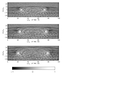
Figure 2.— The evolution of configuration of the inductive electric field during the reconnection process.

3. Electrons heating and acceleration in hot accretion flows

Magnetic reconnection is of course intrinsically a transient process. But in our paper we treat the electron heating/acceleration in reconnection as approximately steady. Specifically, from Figs. 1 & 2 we see that the electromagnetic field almost remains unchanged from t=75 to 125 and reaches a steady state. We investigate the heating/acceleration of electrons during this interval. This approximation is reasonable because the timescale of electron heating/acceleration is very short compared to the timescale of the reconnection process.

Electron dynamics in magnetic reconnection has been previously studied using analytical theories and test particle calculations in different magnetic- and electric-field configurations. (Litvinenko, 1996; Deeg et al., 1991; Browning & Vekstein, 2001; Wood & Neukirch, 2005; Birn & Hesse, 1994). In such studies, the electron orbits are calculated in given electromagnetic fields. Electrons are mainly accelerated by the $\textbf{v}\times\textbf{B}$ reconnection electric field. Liu et al. (2009) performed test-particle simulations of electron acceleration in a reconnecting magnetic field in the context of solar flares, and found that the accelerated electrons present a truncated power-law distribution with an exponential tail at high energies, which is analogous to the case of diffusive shock acceleration.

We use the test-electron method to investigate the acceleration. The electromagnetic fields obtained from 2.5D hybrid simulation of magnetic reconnection is used as the background. One advantage of this method is that it saves a lot of computation time and enables us to perform more calculations.

It is hard to study the electrons movement in the time scale $\Omega^{-1}_{0}$ and space scale $\lambda_{0}$ in hybrid simulation. So the cubic spline interpolation is used to get electric and magnetic fields with higher time resolution ( 0.001 $\Omega^{-1}_{0}$, one step is divided into 100 steps, the step in hybrid simulation is 0.1 $\Omega^{-1}_{0}$), suitable for the calculation for electron dynamics. And we also use the values of electric and magnetic fields on four grids around an electron to calculate the local electric and magnetic fields where the electron locates. The difference method has the following form.

$$F(x,z)=f_{11}(1-dx)(1-dz)+f_{21}(1-dx)dz$$

$$+f_{12}dx(1-dz)+f_{22}dxdz.$$

Here the function $F$ can be any component of the electric and magnetic fields; $f_{11,21,12,22}$ are their values on four grids around the electron; $dx$ and $dz$ are the distance from the electron to the nearest grid in $x$ and $z$ direction, respectively. Such a treatment will rule out artificial high frequency disturbance. The accuracy of such difference method is of second order and also satisfies the requirement of our simulation. The electron movement should satisfy the Newton equation (the relativistic effect is considered):

$$\frac{d\textbf{p}}{dt}=e[\textbf{E}+(\textbf{p}/\gamma)\times\textbf{B}].$$ (5)

Where p is the electron momentum and $\gamma$ is the Lorentz factor.

Figure 3.— The electrons energy distribution before and after acceleration in the case of $\beta_{e}=1.0$. The dotted line denotes the initial (Maxwellian) distribution. The solid line shows the distribution after acceleration. It can be fitted by a new Maxwellian distribution (shown by the dashed line) plus a hard tail.

The size of the simulation box is $[-50\lambda_{0},50\lambda_{0}]\times[-25\lambda_{0},25\lambda_{0}]$. Because of symmetry and in order to reduce the calculation, test electrons are added is in $[0,50\lambda_{0}]\times[0,25\lambda_{0}]$ the region only. The number of the test electrons is 65536. Their initial velocity distribution is Maxwellian and the spacial distribution is homogeneous. The motion of test electrons is controlled by the electric and the magnetic fields obtained in §2.

The resulted new distribution after the acceleration in the case of $\beta_{e}=1.0$ is shown in Figures 3 & 4. We see that the distribution can be described by a new Maxwellian one with higher temperature plus a hard tail which can be fitted by a broken power-law, i.e., the electrons are heated and accelerated after the magnetic reconnection. The temperature of heated electrons increases from $10^{9.30}K$ to $10^{9.65}K$. The broken power-law is described by $dN(E)\propto E^{-p}dE$, with $p=1.47$ between $1$ MeV and $10$ MeV and $p=4$ between $10$ and 40 MeV. Most electrons are heated rather than accelerated, and about $7.94\%$ of the total test electrons are accelerated above 1MeV and $0.93\%$ are accelerated above 10MeV.

Figure 4.— The distribution of accelerated electrons (“hard tail” in Fig. 3) when $\beta=1.0$. It is fitted by a broken power-law.

Figure 5.— The electrons energy distribution before (dot-dot-dot-dashed line) and after acceleration in the cases of $\beta=10.0$ (dashed line), $\beta=0.1$ (dotted line), and $\beta=0.01$ (solid line).

We have also calculated the cases of other values of $\beta_{e}$, density $n_{e}$, and initial electron temperature $T_{e}^{0}$. The results are shown in Figures 5 & 6 and Table 1. We can see that the results are qualitatively similar. Electrons are heated to a higher temperature, and some of them are accelerated. The accelerated electrons can be well described by a broken power-law distribution. When the magnetic field becomes stronger, i.e., $\beta_{e}$ becomes smaller, electrons are more effectively heated and accelerated, namely the “new” temperature becomes higher, and more electrons are accelerated. This implies that more magnetic energy is converted into the kinetic energy of electrons with the increase of the magnetic field. When $\beta$=0.1, some electrons can even be accelerated to more than 5000 MeV. When $\beta$=0.01, however, the magnetic field B is too strong. In this case, the accelerated electrons reaching a certain energy will be deflected by the strong magnetic field and run out of the acceleration region, thus further acceleration is restrained. Although more electrons can be heated to higher temperature and accelerated to higher energy when $\beta$ decreases from 0.1 to 0.01, the highest energy that the electrons can reach when $\beta=0.01$ is smaller than that when $\beta$=0.1. Another interesting result is that the “low-energy” part of the broken power-law, where most accelerated electrons locate, becomes softer with decreasing $\beta_{e}$, with the spectral index $p\sim 0.63,1.47,1.46$ and $1.91$ for $\beta_{e}=10.0,1.0,0.1,$ and $0.01$, respectively.

Table 1Results of electrons acceleration for different initial temperature, density and $\beta e$

$T_{e}^{0}({\rm K})$	$n_{e}({\rm cm}^{-3})$	$\beta_{e}$	$T_{e}$(K)	power-law form		acceleration ratio
$10^{9.3}$	$10^{6}$	10	$10^{9.55}$	$dN(E)\propto E^{-0.63}$(1 -14 MeV)		$2.24\%$(E$\geq$1 MeV)
				$dN(E)\propto E^{-7.59}$(14-23 MeV)		$0.50\%$(E$\geq$10 MeV)
$10^{9.3}$	$10^{6}$	0.1	$10^{9.85}$	$dN(E)\propto E^{-1.46}$(1-17 MeV)		$44\%$(E$\geq$1 MeV)
				$dN(E)\propto E^{-5.05}$(17-46 MeV)		$3.2\%$(E$\geq$10 MeV)
						$0.5\%$(E$\geq$1000 MeV)
$10^{9.3}$	$10^{6}$	0.01	$10^{10.5}$	$dN(E)\propto E^{-1.91}$(5-20 MeV)		$63.1\%$(E$\geq$5 MeV)
				$dN(E)\propto E^{-3.80}$(20-100 MeV)		$28.8\%$(E$\geq$10 MeV)
$10^{9.3}$	$10^{6}$	1	$10^{9.65}$	$dN(E)\propto E^{-1.47}$(1 -10 MeV)		$7.94\%$(E$\geq$1 MeV)
				$dN(E)\propto E^{-4.03}$(10-40 MeV)		$0.93\%$(E$\geq$10 MeV)
$10^{9.3}$	$10^{7}$	1	$10^{9.75}$	$dN(E)\propto E^{-1.63}$(1-10 MeV)		$17.3\%$(E$\geq$1 MeV)
				$dN(E)\propto E^{-3.25}$(10-35 MeV)		$1.1\%$(E$\geq$10 MeV)
$10^{8.5}$	$10^{6}$	1	$10^{9.25}$	$dN(E)\propto E^{-1.69}$(0.5-2.1 MeV)		$5.0\%$(E$\geq$0.5 MeV)
				$dN(E)\propto E^{-4.84}$(2.1-4.5 MeV)		$1.6\%$(E$\geq$1 MeV)

Figure 6.— The distribution of accelerated electrons in the cases of $\beta=10.0$ (solid line), $\beta=0.1$ (dotted line), and $\beta=0.01$ (dash-dotted line). All of them can be fitted by a broken power-law (dashed line).

When the density $n_{e}$ increases (but $\beta_{e}$ and $T_{e}^{0}$ remain the same), the effect is similar to the case of decreasing $\beta_{e}$, namely the electrons are more effectively heated and accelerated. This is because larger density implies stronger magnetic field which is the dominant factor determining the heating and acceleration. When the initial temperature $T_{e}^{0}$ decreases (from $10^{9.3}$K to $10^{8.5}$K) but density and $\beta_{e}$ remain unchanged, we find that the heating and acceleration become less efficient. The “heated” temperature is lower, and less electrons are accelerated. Only a fraction $\sim 5\%$ of electrons can be accelerated to more than 0.5 MeV. This is because a lower $T_{e}^{0}$ corresponds to a weaker magnetic field. But surprisingly, the low-energy part of the power-law distribution becomes softer which seems to indicate that magnetic field is not the only factor determining the acceleration.

4. Summary and Discussion

In this paper we use hybrid simulation code of magnetic reconnection plus test-electron method to study the electrons heating and acceleration by magnetic reconnection process in hot accretion flows. The self-consistent electromagnetic fields are obtained from the hybrid simulation and they are then used in the test-electron calculation. The fiducial parameters of the background accretion flows we adopt are density $n_{e}=10^{6}{\rm cm}^{-3}$ and electron temperature $T_{e}^{0}=2\times 10^{9.3}$K (ions temperature $T_{i}=10T_{e}^{0}$). These values are taken from the accretion flow in Sgr A*, the supermassive black hole in our Galactic center (ref. Yuan et al., 2003). For the strength of the magnetic field in the accretion flow, we set $\beta_{e}(\equiv P_{e}/P_{\rm mag})=1.0$. This is the typical value according to the MHD numerical simulation of hot accretion flow. We find that the electrons are heated and accelerated by the reconnection. The new distribution can be fitted by a Maxwellian distribution plus a broken power-law. The temperature is increased to $10^{9.65}$K and the power-law is described by $dN(E)\propto E^{-1.47}$ between 1 and 10 MeV and $dN(E)\propto E^{-4}$ between 10 MeV and 40 MeV. The fraction of electrons with energy above 1 MeV is $\sim 8\%$. Given that the magnetic field and density in accretion flow are inhomogeneous, we also consider $\beta_{e}=10,0.1$, and $0.01$ and $n_{e}=10^{7}{\rm cm}^{-3}$. We find that the results are qualitatively similar, namely the distribution of electrons can be fitted by a Maxwellian one with a higher “heated” temperature plus a broken power-law. When the magnetic field is stronger ($\beta_{e}$ is smaller or $n_{e}$ is larger), the heating and acceleration become more efficient. The “heated” temperature is higher and more electrons are accelerated. In addition, the “low-energy” part of the broken power-law becomes softer (refer to Table 1).

In our work we assume ideal MHD for the hybrid simulation, thus the Joule heating to the accretion flow is neglected. Obviously the electrons will be heated to a higher temperature when this effect is considered.

References

- Baganoff et al. (2001) Baganoff, F. K., et al. 2001, Nature, 413, 45
- Baker et al. (2002) Baker, D. N. 2002, Geophys. Res. Lett., 29, 43
- Balbus & Hawley (1991) Balbus, S.A., & Hawley, J.F. 1991, ApJ, 376, 214
- Bieber et al. (1982) Bieber, J. W., Stone, E. C., Hones, E. W., Baker, D. N., & Bame, S. J. 1982, Geophys. Res. Lett., 9, 664
- Birn & Hesse (1994) Birn, J., & Hesse, M. 1994, J. Geophys. Res., 99, 109
- Bisnovatyi-Kogan & Lovelace (1998) Bisnovatyi-Kogan, G.S. & Lovelace, R.V.E. 1998, ApJ, 486, L43
- Browning & Vekstein (2001) Browning, K., & Vekstein, G. E. 2001, J. Geophys. Res., 106, 18677
- Cargill & Klimchuk (1997) Cargill, P. A., & Klimchuk, J. A. 1997, ApJ, 478, 799
- Deeg et al. (1991) Deeg, H. J., Borovsky, J., & Duric, N. 1991, Phys. Fluids B, 3, 2660
- Dodds-Eden et al. (2009) Dodds-Eden, K., et al. 2009, ApJ, 698, 676
- Drake et al. (2005) Drake, E. N., Shay, M. A., Thongthai, W. 2005, Phys. Rev. Lett., 94, 095001
- Eckart et al. (2006) Eckart, A., et al. 2006, A&A, 455, 1
- Eckart et al. (2009) Eckart, A., et al. 2009, A&A, 500, 935
- Goodman & Uzdensky (2008) Goodman, J., & Uzdensky, D. 2008, ApJ, 688, 555
- Hawley & Balbus (2002) Hawley, J. F., & Balbus, S. A. 2002, ApJ, 573, 738
- Heyvaerts et al. (1988) Heyvaerts, J., Norman, C., & Pudritz, R. E. 1988, ApJ, 330, 718
- Hirose et al. (2004) Hirose, S., Krolik, J., De Villiers, J-P., & Hawley, J. 2004, ApJ, 606, 1083
- Hornstein et al. (2007) Hornstein, S. D., et al. 2007, ApJ, 667, 900
- Karlicky (2008) Marian Karlicky, 2008, ApJ, 674, 1211
- Larrabee et al. (2003) Larrabee, D. A., Lovelace, R. V. E., & Romanova, M. M. 2003, ApJ, 586, 72
- Litvinenko (1996) Litvinenko, Y. E. 1996, ApJ, 462, 997
- Liu et al. (2009) Liu, W. J., Chen, P. F., Ding, M. D., & Fang, C. 2009, ApJ, 690, 1633
- Lyutikov (2003) Lyutikov, M. 2003, New Astronomy Review, 47, 513
- Machida & Matsumoto (2003) Machida, M., & Matsumoto, R. 2003, ApJ, 585, 429
- Michel (1994) Michel, F. C. 1994, ApJ, 431, 397
- Parker (1958) Parker, E. N. 1958, J. Geophys. Res., 62, 509
- Parker (1963) Parker, E. N. 1963, ApJ, 8, 177
- Quataert & Gruzinov (1999) Quataert, E., & Gruzinov, A. 1999, ApJ, 520, 248
- Schopper et al. (1998) Schopper, R., Lesch, H., & Birk, G. T. 1998, A&A, 335, 26
- Somov & Kosugi (1997) Smov, B. V., & Kosugi, T. 1997, ApJ, 485, 859
- Swift (1995) Swift, D. W. 1995, Geophys. Res. Lett., 22, 311
- Swift (1996) Swift, D. W. 1996, J. comput. phys., 126, 109
- Tsiklauri & Haruki (2007) Tsiklauri, D., & Haruki, T. 2007, Physics of Plasmas, Volume 14, Issue 11, pp. 112905-112905-10
- Uzdensky & Goodman (2008) Uzdensky, D., & Goodman, J. 2008, ApJ, 682, 608
- Wood & Neukirch (2005) Wood, P., & Neukirch, T. 2005, Sol. Phys., 226, 73
- Yuan et al. (2009) Yuan, F., Lin, J., Wu, K. & Ho, L. 2009, MNRAS, 395, 2183
- Yuan et al. (2003) Yuan, F., Quataert, E., & Narayan, R. 2003, ApJ, 598, 301
- Yuan et al. (2004) Yuan, F., Quataert, E., & Narayan, R. 2004, ApJ, 606, 894
- Zenitani & Hoshino (2007) Zenitani, S., & Hoshino, M. 2007, ApJ, 670, 702