Bosonization of one dimensional fermions out of equilibrium

Abstract

Bosonization technique for one-dimensional fermions out of equilibrium is developed in the framework of the Keldysh action formalism. We first demonstrate how this approach is implemented for free fermions and for the problem of non-equilibrium Fermi edge singularity. We then employ the technique to study an interacting quantum wire attached to two electrodes with arbitrary energy distributions. The non-equilibrium electron Green functions, which can be measured via tunneling spectroscopy technique and carry the information about energy distribution, zero-bias anomaly, and dephasing, are expressed in terms of functional determinants of single-particle “counting” operators. The corresponding time-dependent scattering phase is found to be intrinsically related to “fractionalization” of electron-hole excitations in the tunneling process and at boundaries with leads. Results are generalized to the case of spinful particles as well to Green functions at different spatial points (relevant to the problem of dephasing in Luttinger liquid interferometers). For double-step distributions, the dephasing rates are oscillatory functions of the interaction strength.

I Introduction

One-dimensional (1D) interacting fermionic systems show remarkable physical properties. The electron-electron interaction manifests itself in a particularly dramatic way in 1D systems, inducing a strongly correlated electronic state – Luttinger liquid (LL) Gogolin ; stone ; giamarchi ; maslov-lectures ; Delft . A paradigmatic experimental realization of quantum wires are carbon nanotubes zba-carbon-nanotubes ; for a recent review see Ref. nanotubes, . Further realizations encompass semiconductorsemiconductor , metallic metallic and polymer nanowirespolymer , as well as quantum Hall edgesHall ; MachZehnder .

While equilibrium LL have been extensively explored, there is currently a growing interest in non-equilibrium phenomena on nanoscale and, in particular, in non-equilibrium properties of quantum wires. In a recent experiment Chen09 the tunneling spectroscopy of a biased LL conductor has been performed (see also a related work on carbon nanotube quantum dots dirks09 ). A similar approach was used to study experimentally non-equilibrium quantum Hall edges altimiras09 . Quite generally, the tunneling spectroscopy technique allows one to measure the non-equilibrium Green functions $G^{\gtrless}(\tau)$. Analogous experiments Pothier have been carried out earlier in order to study energy distribution function and inelastic relaxation processes in quasi-one-dimensional diffusive metallic samples. The interpretation of the results for a metallic sample is based on the Fermi liquid theory, and, in particular, on a kinetic equation for a quasi-particle distribution function. In fact, even in that case, careful analysis requires taking into account non-equilibrium dephasing processes GGM which lead to additional broadening of the measured Fermi-edge structures in the tunneling current. In the case of strongly correlated, non-Fermi-liquid systems (such as LL) out of equilibrium, the situation is much more complex. In this situation not only a quantitative theoretical analysis of $G^{\gtrless}$, but even the very notions of quasiparticle energy distribution and dephasing, become highly non-trivial. The goal of the presented work is to construct a corresponding theory. To achieve this goal, we develop a formalism of non-equilibrium (Keldysh) bosonization. While we consider systems of 1D interacting electrons in this work, we expect that it will be an important step in understanding the properties of a broader class of systems—non-equilibrium quantum fluids in low-dimensions. This includes, in particular, systems of cold atoms, with either fermionic or bosonic statistics.

The structure of the present paper is as follows:

In Sec. II we discuss possible experimental realizations of a non-equilibrium LL.

In Sec. III we develop a bosonization technique for non-interacting electrons away from equilibrium. Working within the Keldysh non-equilibrium formalism, we derive the action of the bosonized theory. While this action is quadratic at equilibrium (which is the essence of conventional bosonization), it now includes arbitrary powers in the bosonic fields. We demonstrate how this action can be used to express the Green function of non-interacting fermions in terms of a Fredholm functional determinant of a single-particle “counting” operator (which is of Toeplitz type). We further discuss the relation between this problem and that of counting statistics. Specifically, our result is expressed in terms of the determinant at the value of the phase (“counting field”) $\lambda=2\pi$. On the other hand, the counting statistics at this point is trivial, in view of charge quantization. We show that the difference between the determinants used for expressing the Green functions and those used for counting statistics results from different continuations (analytic vs. periodic) of the functional determinant beyond the non-analyticity point $\lambda=\pi$.

In Sec. IV we apply our technique to the problem of Fermi edge singularity (FES) out of equilibrium. We show that non-equilibrium FES Green function is expressed in terms of the same functional determinant but with a shifted value of the argument, $\lambda=2(\pi-\delta_{0})$ , where $\delta_{0}$ is the scattering phase on the core hole. Comparing our results for this problem with those obtained earlierAbanin , we establish useful identities between Fredholm determinants of counting operator at values of the counting field $\lambda$ differing by $2\pi$.

In Sec.V our formalism is extended to interacting fermions in a quantum wire. First, we analyze the problem of tunneling spectroscopy of a non-equilibrium LL in the case of spinless fermions. We demonstrate that the non-equilibrium Green functions are expressed in terms of products of single-particle Fredholm determinants. The corresponding values of the counting fields are shown to be related to “fractionalization” of particle-hole excitations created during the tunneling process, as well as at the boundaries with non-interacting leads. Our results for $G^{\gtrless}$ contain all information about single-particle properties of the system, including tunneling density of states, energy distribution, and dephasing. We find, in particular, that the dephasing rate oscillates as a function of the interaction strength (LL parameter $K$), vanishing at certain values of $K$. At the end of the section we generalize the consideration to the case of spinful fermions, as well to Green functions at different spatial points (which is relevant to the problem of dephasing in LL interferometers).

Section VI includes a summary of our results as well as prospects for future work.

Some of results of this work were presented in a Letter, Ref. GGM_2009_short, .

II Nonequilibrium Luttinger liquid: Setups

In this section we specify the class of problems to be considered and discuss possible experimental setups. We assume that electrons with distributions functions $n_{\eta}(\epsilon)$ ($\eta=R,L$ labels right- and left-movers) are injected into a LL wire from two non-interacting electrodes. It is convenient to model the electrodes as non-interacting 1D systems, so that the whole structure is a wire with spatially dependent interaction that switches on near the points $x=\pm L/2$, see Sec. V for detail.

It is worth noting that we assume the absence of electron backscattering due to impurities inside the LL wire. When present in sufficient amount (so that one can speak about a disordered LL), such impurities strongly affect the electronic properties of a LL wire. Specifically, they induce diffusive dynamics at sufficiently high temperature $T$ and localization phenomena proliferating with lowering $T$ (Ref. Apel82, ; Giamarchi, ; GMP, ), as well as inelastic processes Bagrets1 . We also neglect the nonlinearity of the electron dispersion whose influence on spectral and kinetic properties of 1D electrons was recently studied in Refs. khodas, , Matveev, .

We discuss now possible experimental realizations of the problem. The simplest way to take the system out of equilibrium is to apply a voltage between two electrodes, so that the incoming distribution functions have different chemical potentials, $\mu_{L}-\mu_{R}=eV$, but equal temperatures, $T_{R}=T_{L}=T$, see e.g. Ref. Chudnovsky, . However, in the case of a LL this situation is almost identical to the equilibrium one, in view of the absence of electron backscattering. Indeed, the bosons remain at equilibrium, so that the usual bosonization technique (within Matsubara formalism) can be applied. The only non-equilibrium effect will be a simple shift of the chemical potential of left- movers as compared to that of the right-movers.

A generalization of this setup that does yield a non-trivially non-equilibrium LL is shown in Fig. 1a. A long clean LL is adiabatically coupled to two electrodes with different potentials, $\mu_{L}-\mu_{R}=eV$ and different temperatures $T_{L}$, $T_{R}$. (A particularly interesting situation arises when one of temperatures is much larger than the other, e.g., $T_{L}=0$ and $T_{R}$ finite, so that non-equilibrium effects are most pronounced.) This model has been investigated in our previous works, Refs. GGM2008, ; GGM_2009, . While showing genuinely non-equilibrium effects (in particular, energy redistribution of electrons), this model, when treated in the framework of Keldysh bosonization formalism, is characterized by a Gaussian action. For this reason, we termed this setup “partially non-equilibrium” in Ref. GGM2008, . We will verify in Sec.V that the results of the present work (pertaining to full non-equilibrium) reduce to those obtained earlier (partial non-equilibrium) in the case when both $n_{R}$ and $n_{L}$ are taken to be Fermi-Dirac functions.

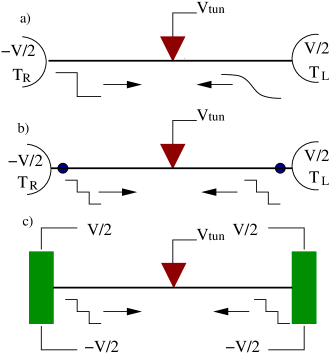
Figure 1: Schematic view of experimental setups for tunneling spectroscopy of a LL out of equilibrium: (a) “partially non-equilibrium” setup, with distribution functions $n_{\eta}(\epsilon)$ of Fermi-Dirac form but with different temperatures; (b), (c) “fully non-equilibrium” setups characterized by double-step distribution functions $n_{\eta}(\epsilon)$ of electrons injected into the LL wire.

The focus of this work is generic non-equilibrium situations, when at least one of the functions $n_{\eta}$ is not of the Fermi-Dirac form. Such situations naturally arise when electrons injected into a LL wire represent juxtaposition of particles originating from reservoirs with different chemical potentials and mixed by impurity scattering. Two possible realizations of such devices are shown in Fig. 1b,c. In the first case, Fig. 1b, the mixture of left and right movers coming from reservoirs with $\mu_{L}\neq\mu_{R}$ is caused by impurities which are located in the non-interacting part of the wires Ngo . In the second setup, Fig. 1c, the LL wire is attached to two thick metallic wires which are themselves biased. We assume that those electrodes are diffusive but sufficiently short, so that energy equilibration there can be neglected. As a result, a double-step energy distribution is formed in the electrodes Pothier and “injected” into the LL conductor. Such double-step distributions are of particular interest for our problem, as they are of the “maximally non-equilibrium” form. The existence of multiple Fermi edges in the distribution functions “injected” from the electrodes renders the electron-electron scattering processes GGM ; Altland which govern the non-equilibrium dephasing rate $\tau_{\phi}$ (and thus the broadening of tunneling spectroscopy characteristics) particularly important.

The question of non-equilibrium dephasing induced by electron-electron scattering is particularly intriguing in the case of a 1D system. First, energy relaxation is absent in a homogeneous LL system. Second, recent analysis of dephasing in the context of weak localization and Aharonov-Bohm oscillations has given qualitatively different results: while the weak-localization dephasing rate vanishes in the limit of vanishing disorder GMP , the Aharonov-Bohm dephasing rate is finite in a clean LL GMP ; lehur . In the case of a partially non-equilibrium setup the tunneling spectroscopy dephasing rate has a form similar to the equilibrium Aharonov-Bohm dephasing rate GGM2008 ; GGM_2009 . As we show here, in the case of double-step distributions dephasing acquires qualitatively distinct features; in particular, the dephasing rate becomes an oscillatory function of the interaction strength.

Having described the problems to be addressed, we turn to the corresponding formalism. It is instructive to develop it first for the case of non-interacting fermions and then “turn on” the interaction.

III Free fermions

In this section we develop a bosonization formalism for the case of free fermions out of equilibrium. Specifically, we consider non-interacting fermions with a given distribution function $n(\epsilon)$ and derive the corresponding bosonic action. Using the latter, we calculate the fermionic Green function. Clearly, the Green function of non-interacting fermions is trivially obtained within the fermionic formalism. However, the results of this section are not just a complicated way to calculate a simple quantity. Rather, they will play a crucial role for developing the bosonic formalism for interacting systems studied in the remainder of the paper.

III.1 Keldysh action: From fermions to bosons

Bosonization has been proved to be a very efficient tool for tackling one dimensional problems at equilibriumGogolin ; stone ; giamarchi ; maslov-lectures ; Delft , as it maps a system of interacting fermions (LL) onto that of non-interacting bosons. One can thus hope for similar advantages of this approach for non-equilibrium problems as well. The question though is whether the bosonization procedure can be generalized to systems out of equilibrium? As we show below, the answer is affirmative, yet substantial modifications are required.

Quite generally, operator bosonization procedure consists of the following steps: (i) mapping between the Hilbert space of fermions and bosons; (ii) construction of the bosonic Hamiltonian $H_{B}$ representing the original fermionic Hamiltonian $H_{F}$ in terms of bosonic (particle-hole) excitations, i.e. density fields; (iii) expressing fermionic operators in the bosonic language; (iv) calculation of observables (Green functions) within the bosonized formalism by averaging with respect to the many body bosonic density matrix (${\rho}_{B}$). Neither the Hilbert space nor the operators (including the Hamiltonian) contain an information regarding a state of the many-body system. Therefore, the first three steps remain unchanged for a non-equilibrium situation. The major modifications occur in the step (iv). Indeed, at equilibrium the fermionic density matrix is expressed through the corresponding Hamiltonian as $\rho_{F}=\exp(-H_{F}/T)$, implying that the same relation holds in the bosonized theory, $\rho_{B}=\exp(-H_{B}/T)$, which makes averaging with respect to $\rho_{B}$ straightforward. Out of equilibrium this is not so anymore: a one-particle density matrix corresponding to a non-equilibrium occupation $n(\epsilon)$ of fermionic states translates into a complicated density matrix of bosons, which does not allow the application of Wick theorem. This poses a major difficulty in bosonizing fermionic problems away from equilibrium and, as we see below, results in a non-gaussian action of the bosonized theory.

To construct the effective bosonic theory, we start with the fermionic description. Within the LL model, the electron field is decoupled into a sum of left- and right-moving terms,

$$\psi(x,t)=\psi_{R}(x,t)e^{ip_{F}x}+\psi_{L}(x,t)e^{-ip_{F}x}\,,$$ (1)

where $p_{F}$ is the Fermi momentum. The Hamiltonian of the system reads

$$H_{0}=-iv\int dx\left(\psi_{R}^{\dagger}\partial_{x}\psi_{R}-\psi^{\dagger}_{L}\partial_{x}\psi_{L}\right)\,,$$ (2)

where $v$ is the electron velocity. The bosonic representation for fermionic operators has the form Gogolin ; stone ; giamarchi ; maslov-lectures ; Delft ; Klein_factors

$$\psi_{\eta}(x)\simeq\left(\frac{\Lambda}{2\pi v}\right)^{1/2}e^{\eta ip_{F}x}e^{i\phi_{\eta}(x)}\,,$$ (3)

where $\Lambda$ is an ultraviolet cut-off. The bosonic fields $\phi_{\eta}(x)$ are related to the density of electrons (given by $\rho_{\eta}(x)=\psi_{\eta}^{\dagger}(x)\psi_{\eta}(x)$ in the fermionic language) as

$$\rho_{\eta}(x)=\frac{\eta}{2\pi}\partial_{x}\phi_{\eta}\,,$$ (4)

and obey the commutation relations

$$[\phi_{R}(x),\phi_{R}(x^{\prime})]=-[\phi_{L}(x),\phi_{L}(x^{\prime})]=i\pi{\operatorname{sgn}}(x-x^{\prime})\,.$$ (5)

We use the convention that in formulas $\eta$ should be understood as $\eta=\pm 1$ for right/left moving electrons. The bosonized Hamiltonian is expressed in terms of density fields in the following way:

$$H_{0}=\pi v\int dx\left(\rho_{R}^{2}+\rho_{L}^{2}\right)\,.$$ (6)

We turn now to the Lagrangian formalism. Since we deal with a non-equilibrium situation, the system is characterized by an action defined on the Keldysh contourKamenev ,

$$S_{0}[\psi]=\int_{c}dt\int dx\sum_{\eta=R,L}\psi^{\dagger}_{\eta}i\partial_{\eta}\psi_{\eta}$$ (7)

where $\psi,\psi^{\dagger}(t,x)$ are fermionic fields, and $\partial_{R,L}=\partial_{t}\pm v\partial_{x}$. To generate correlation functions, it is convenient to introduce a source term.

$$S_{V}[\psi]=\int_{c}dt\int dxV_{\eta}(x,t)\psi_{\eta}^{\dagger}(x,t)\psi_{\eta}(x,t)\,.$$ (8)

The field components on the upper branch and lower are denoted by $+$ and $-$ respectively. It is convenient to perform a rotation in Keldysh spaceKamenev , thus decomposing fields into classical and quantum components (the latter being denoted by a bar),

$$V_{\eta},\bar{V}_{\eta}=(V_{+,\eta}\pm V_{-,\eta})/\sqrt{2}\,,$$ (9)

$$\rho_{\eta},\bar{\rho}_{\eta}=(\rho_{+,\eta}\pm\rho_{-,\eta})/\sqrt{2}\,,$$ (10)

$$\psi_{\eta},\bar{\psi}_{\eta}=(\psi_{+,\eta}\pm\psi_{-,\eta})/\sqrt{2}\,,$$ (11)

$$\psi^{\dagger}_{\eta},\bar{\psi}_{\eta}^{\dagger}=(\psi^{\dagger}_{+,\eta}\mp\psi^{\dagger}_{-,\eta})/\sqrt{2}\,.$$ (12)

In these notations, the density correlation functions are encoded in the generating function

$${Z}_{\eta}[V_{\eta},\bar{V}_{\eta}]=\langle\exp\{iV_{\eta}\bar{\rho}_{\eta}+i\bar{V}_{\eta}\rho_{\eta}\}\rangle_{S_{0}}\,.$$ (13)

The calculation of the partition function can be performed in either the fermionic or the bosonic description. In the fermionic language it can be readily done by evaluating a Gaussian integral over the Grassman variables,

$${Z}_{\eta}[V,\bar{V}]={\mathrm{det}}[1+G_{\eta 0}(\sigma_{0}V+\sigma_{1}\bar{V})/\sqrt{2}]\,,$$ (14)

where $\sigma_{0}$ and $\sigma_{1}$ are the unit matrix and the first Pauli matrix in the Keldysh space, and $G_{\eta 0}$ is the Keldysh Green function of free chiral fermions, which has the following matrix structure:

$$G_{\eta 0}=\begin{pmatrix}G^{r}_{\eta 0}&G^{K}_{\eta 0}\\ 0&G^{a}_{\eta 0}\end{pmatrix}\>\!.$$ (15)

Here $G^{a}_{\eta,0}$, $G^{r}_{\eta,0}$ and $G^{K}_{\eta,0}$ are advanced, retarded and Keldysh components,

$$G_{\eta 0}^{r,a}(\epsilon,p)=1/(\epsilon-\eta vp\pm i0)\,;$$ (16)

$$G_{\eta 0}^{K}(\epsilon,p)=[1-2n_{\eta}(\epsilon)][G_{\eta 0}^{r}(\epsilon,p)-G_{\eta 0}^{a}(\epsilon,p)]\,.$$ (17)

We expand now the generating functional (14) in powers of the source fields $V_{\eta}$, $\bar{V}_{\eta}$. For higher-dimensional systems this would generate all terms of the type $V_{\eta}^{n}\bar{V}_{\eta}^{m}$. In 1D the situation is different. Specifically, in an equilibrium 1D system only terms up to second order ($V_{\eta}\bar{V}_{\eta}$ and $\bar{V}_{\eta}^{2}$) are generated, which forms the basis of conventional bosonization. Out of equilibrium, this is not true anymore: terms of higher orders are generated as well, and the theory becomes non-gaussian. What is crucial, however, is that all higher-order terms are of the type $\bar{V_{\eta}}^{n}$, i.e. they do not depend on $V_{\eta}$. We will prove this statement in Sec. III.2 and III.3 below.

The generating functional has thus the structure

$${Z}_{\eta}[V,\bar{V}]=\exp\left(-iV_{\eta}\Pi^{a}_{\eta}\bar{V}_{\eta}+\sum_{n=2}^{\infty}\frac{i^{n}}{n!}\bar{V}_{\eta}^{n}{\cal S}_{n,\eta}\right)\,,$$ (18)

where ${\cal S}_{n,\eta}$ is the $n$-th order irreducible vertex function,

$${\cal S}_{n,\eta}(x_{1},t_{1};\ldots;x_{n},t_{n})$$

$$\qquad=-i^{n}\sum_{\rm perm.}{\mathrm{Tr}}_{K}G_{\eta 0}(x_{1},t_{1};x_{i_{2}},t_{i_{2}}){\sigma_{1}\over\sqrt{2}}$$

$$\qquad\times G_{\eta 0}(x_{i_{2}},t_{i_{2}};x_{i_{3}},t_{i_{3}}){\sigma_{1}\over\sqrt{2}}\times\ldots$$

$$\qquad\times G_{\eta 0}(x_{i_{n}},t_{i_{n}};x_{1},t_{1}){\sigma_{1}\over\sqrt{2}}\,.$$ (19)

The multiplication in Eq. (18) and analogous formulas below should be understood in the matrix sense with respect to the coordinates,

$$V_{\eta}\Pi^{a}_{\eta}\bar{V}_{\eta} = \int[dx][dt]V_{\eta}(x_{1},t_{1})$$

$$\times \Pi^{a}_{\eta}(x_{1},t_{1};x_{2},t_{2})\bar{V}_{\eta}(x_{2},t_{2})\,,$$

$$\bar{V}_{\eta}^{n}{\cal S}_{n,\eta} = \int[dx][dt]\bar{V}_{\eta}(x_{1},t_{1})\dots\bar{V}_{\eta}(x_{n},t_{n})$$ (21)

$$\times {\cal S}_{n,\eta}(x_{1},t_{1};\dots;x_{n},t_{n})\,,$$

where $\int[dx][dt]$ implies integration over all spatial and time coordinates. The summation in Eq. (III.1) goes over $(n-1)!$ permutations $\{i_{2},i_{3},\ldots,i_{n}\}$ of the set of indices $\{2,\ldots,n\}$ (labeling the space-time coordinates), and ${\rm Tr}_{K}$ denotes the trace over Keldysh indices. Clearly, after integration with $\bar{V}_{\eta}$ fields in Eq. (18) all the $(n-1)!$ terms of the sum in Eq. (III.1) yield equal contributions, so that the total combinatorial factor is $(n-1)!/n!=1/n$, as should be in the expansion of the logarithm. We have chosen to define the vertex function in the symmetrized form (III.1) [and to introduce the corresponding factor $1/(n-1)!$ in Eq. (18)], since ${\cal S}_{n,\eta}(x_{1},t_{1};\ldots;x_{n},t_{n})$ are then equal to irreducible density correlation functions $\langle\langle\rho(x_{1},t_{1})\ldots\rho(x_{n},t_{n})\rangle\rangle$.

The quadratic part of the generating functional (18) is determined by the polarization operator of fermions,

$$\Pi_{\eta}=\begin{pmatrix}0&\Pi^{a}_{\eta}\\ \Pi^{r}_{\eta}&\Pi^{K}_{\eta}\end{pmatrix},$$ (22)

with the retarded, advanced, and Keldysh components given by

$$\Pi^{r,a}_{\eta}(\omega,q)=\frac{1}{2\pi}\frac{\eta q}{\eta vq-\omega\mp i0},$$ (23)

$$\Pi^{K}_{\eta}(\omega,q)=[\Pi^{r}_{\eta}(\omega,q)-\Pi^{a}_{\eta}(\omega,q)]B_{\eta}(\omega)\,.$$ (24)

Here the function

$$B_{\eta}(\omega)=\frac{1}{\omega}\int_{-\infty}^{\infty}d\epsilon\>n_{\eta}(\epsilon)\>[2-n_{\eta}(\epsilon-\omega)-n_{\eta}(\epsilon+\omega)],$$ (25)

governs the distribution function $N_{\eta}(\omega)$ of electron-hole excitations moving with velocity $v$ in direction $\eta$, $B_{\eta}(\omega)=1+2N_{\eta}(\omega)$. At equilibrium,

$$B_{\eta}(\omega)=B_{\rm eq}(\omega)=1+2N_{\rm eq}(\omega)=\coth\left(\frac{\omega}{2T}\right)\,,$$ (26)

where $N_{\rm eq}(\omega)$ is the Bose distribution. By construction, the second order density-correlation function ${\cal S}_{\eta,n=2}$ in Eq. (18) is equal to the Keldysh component $\Pi_{\eta}^{K}$ of the polarization operator (times $-i$).

In order to bosonize the theory, we should find a bosonic counterpart of the action $S_{0\eta}$ that reproduces the generating functional (18). According to Eq. (13), we have

$$\exp\left(iS_{0\eta}[\bar{\rho}_{\eta},\rho_{\eta}]\right)=\int{\cal D}V_{\eta}{\cal D}\bar{V}_{\eta}{Z}_{\eta}[V_{\eta},\bar{V}_{\eta}]e^{-iV_{\eta}\bar{\rho}_{\eta}-i\bar{V}_{\eta}\rho_{\eta}}\,.$$ (27)

Substituting Eq. (18) into Eq. (27), we obtain the bosonized action

$$S_{0\eta}[\rho_{\eta},\bar{\rho}_{\eta}]=\rho_{\eta}\Pi^{a^{-1}}_{\eta}\bar{\rho}_{\eta}-i\ln Z_{\eta}[\bar{\chi}].$$ (28)

Here $Z_{\eta}[\bar{\chi}]\equiv Z_{\eta}[\chi=0,\bar{\chi}]$ is a partition function (18) of free fermions,

$$i\ln Z_{\eta}[\bar{\chi}]=\sum_{n=2}^{\infty}i^{n+1}\bar{\chi_{\eta}}^{n}{\cal S}_{n,\eta}/n!\,,$$ (29)

subject to the external quantum field

$$\bar{\chi}_{\eta}=\Pi_{\eta}^{a^{-1}}\bar{\rho}_{\eta}\,.$$ (30)

The combined action of left- and right-moving electrons is simply given by a sum of the corresponding chiral actions,

$$S_{0}[\rho,\bar{\rho}]=\sum_{\eta}S_{0\eta}[\rho_{\eta},\bar{\rho}_{\eta}]\,.$$ (31)

Thus we have described a system of non-equilibrium free fermions by a bosonic theory, Eq.(31). In this approach information on the non-equilibrium state of the system is encoded in the vertices (${\cal S}_{n\eta}$), schematically depicted in Fig.2. In Sec. III.2 we discuss the status and implications of the Dzyaloshinskii-Larkin theorem concerning these vertices.

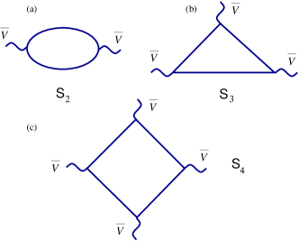
Figure 2: Vacuum loops for free fermions in an external field $\bar{V}$. At equilibrium only ${\cal S}_{2}$ is non-zero, according to the Dzyaloshinskii-Larkin theorem. Away from equilibrium, all vertices appear. For details see Sec. III.2.

III.2 Dzyaloshinskii-Larkin theorem

The appearance of higher-order ($n>2$) fermionic vertices may seem to contradict the Dzyaloshinskii-Larkin theoremDzLar:73 . The latter states that diagrams containing closed loops with more than two fermionic lines vanish. Although the theorem was formulated for the equilibrium case, its proof, given in Ref. DzLar:73, , ostensibly relies solely on particle conservation. Since the latter remains valid out of equilibrium, one might expect the theorem to hold under non-equilibrium conditions as well. To understand why Dzyaloshinskii-Larkin theorem is in fact restricted to the equilibrium case only, and what its implications for a non-equilibrium situation are, we carefully re-examine the arguments of Ref. DzLar:73, .

One starts with the continuity equation for the chiral current and density operators,

$$\omega{\rho}_{\eta}-\eta q{j}_{\eta}=0\,.$$ (32)

Since within the LL model these operators are related to each other through $j_{\eta}=\eta v\rho_{\eta}$, the continuity equation can be rewritten in terms of the density field only,

$$(\omega-\eta vq){\rho}_{\eta}=0\,.$$ (33)

As a consequence, correlation functions of densities satisfy

$$(\omega_{i}-\eta vq_{i})\langle{\rho}_{\eta}(\omega_{1},q_{1}){\rho}_{\eta}(\omega_{2},q_{2})\dots\rho_{\eta}(\omega_{n},q_{n})\rangle=0$$ (34)

for any $i=1,\ldots,n$. Therefore, the irreducible density correlation functions ${\cal S}_{n\eta}(\omega_{1},q_{1};\omega_{2},q_{2};\dots\omega_{n},q_{n})$ with $n>2$ should be zero everywhere, except possibly for the mass shell with respect to all argumentsnote-DL ,

$${\cal S}_{n\eta}(\omega_{1},q_{1};\omega_{2},q_{2};\dots\omega_{n},q_{n})=$$

$$=\delta(\omega_{1}-\eta vq_{1})\delta(\omega_{2}-\eta vq_{2})\ldots\delta(\omega_{n}-\eta vq_{n})$$

$$\times{\cal S}_{\eta}(\omega_{1},\omega_{2},\dots,\omega_{n})\delta(\omega_{1}+\ldots+\omega_{n}).$$ (35)

In the case $n=2$ the argument is not applicable in view of the Schwinger anomaly, yielding the first term in the exponent on the r.h.s. of Eq. (18). When translated into the coordinate-time space, the mass-shell condition (III.2) implies that the correlation function depends in fact only on the world line to which each of the points $(t_{i},x_{i})$ belongs but not on the position of this point on the line:

$${\cal S}_{n\eta}(t_{1},x_{1};\ldots;t_{n},x_{n}) \equiv \langle\langle{\rho}_{\eta}(t_{1},x_{1})\ldots{\rho}_{\eta}(t_{n},x_{n})\rangle\rangle$$

$$= \langle\langle{\rho}_{\eta}(0,\xi_{1})\ldots{\rho}_{\eta}(0,\xi_{n})\rangle\rangle,$$

where $\xi_{i}=x-\eta vt_{i}$. In the Keldysh formalism language, the only non-zero irreducible density correlation function in any order $n>2$ arises when one considers the correlator with all $n$ fields being the classical components $\rho$. (This follows from the fact that the operators $\rho$ commute to a c-number.) These correlation functions are the noise cumulants in the system.

The behavior of the correlation functions ${\cal S}_{n\eta}$ on the “light cone” (III.2) can not be determined from particle conservation law and requires an additional calculation. While at equilibrium all ${\cal S}_{n\eta}$ with $n>2$ do vanish (which reconciles our theory with the Larkin-Dzyaloshinskii theorem), out of equilibrium they are in general non-zero. We consider this general situation in Sec. III.3 where we show that the bosonized action can be presented in a compact form of a functional determinant.

III.3 Bosonized action as functional determinant

As we have shown, the bosonic action, Eq. (31), is expressed through the partition function $Z[V,\bar{V}]$ of free fermions in an external field $V(x,t)$ defined on the Keldysh contour. In one dimension the partition function can be cast in a relatively simple form. To achieve this, we first present the partition function

$$Z[V,\bar{V}]={\mathrm{tr}}\{\rho_{F}S_{c}\}\,.$$ (37)

Here $S_{c}$ is an evolution operator along Keldysh contour,

$$Z[V,\bar{V}] = \lim_{t\rightarrow\infty}{\mathrm{tr}}\{\rho_{F}e^{-iH[V_{+}(-t)]\Delta t}e^{-iH[V_{+}(-t+\Delta t)]\Delta t}$$ (38)

$$\times \ldots\times e^{-iH[V_{+}(t)]\Delta t}e^{iH[V_{-}(t)]\Delta t}e^{iH[V_{-}(t-\Delta t)]\Delta t}$$

$$\times \ldots\times e^{iH[V_{-}(-t)]\Delta t}\}\,,$$

and the trace is taken over the many-body fermionic Fock space. Equation (38) can be further simplified by means of the following identityKlich

$${\mathrm{tr}}\{e^{H_{1}}e^{H_{2}}\dots e^{H_{N}}\}={\mathrm{det}}(1+e^{h_{1}}e^{h_{2}}\dots e^{h_{N}})\,.$$ (39)

Here $h_{n}$ is a matrix in the single particle Hilbert space, and

$$H_{n}=\sum_{i,j}h_{n}^{i,j}a^{\dagger}_{i}a_{j}$$ (40)

is the corresponding operator quadratic in fermionic creation/annihilation operators ($a^{\dagger},a$). The trace in the l.h.s. of Eq.(39) is taken in the many-body Fock space, while the determinant on the r.h.s. is taken in the single-particle space.

Applying Eq.(39) in the continuum limit, we express the partition function in the following form

$$Z_{\eta}[V_{\eta},\bar{V}_{\eta}]={\mathrm{det}}[1-{n}_{\eta}+{n}_{\eta}U_{+,\eta}^{-1}U_{-,\eta}]\,.$$ (41)

Here

$$U_{+,\eta}(t)=\mathrm{Texp}\left(-i\int_{0}^{t}dt{h}_{+,\eta}\right)\,,$$

$$U_{-,\eta}^{-1}(t)=\mathrm{\tilde{T}exp}\left(i\int_{0}^{t}dt{h}_{-,\eta}\right)\,$$ (42)

are evolution operators that correspond to the single-particle Hamiltonians

$${h}_{+,\eta}=-i\eta v\frac{\partial}{\partial x}+V_{+}(x,t)\,,$$

$${h}_{-,\eta}=-i\eta v\frac{\partial}{\partial x}+V_{-}(x,t)\,.$$ (43)

Thus the many-body problem of summing all vacuum loops has been reduced to a calculation of a functional determinant of an operator in a single-particle Hilbert space. To simplify it further, we analyze the properties of the evolution operator $U$ in one dimension. Its action on a wave function $\psi(x)$ can be described as

$$\psi(x,t)=\mathrm{Texp}\left(-i\int_{0}^{t}dt{h}_{+}\right)\psi(x,0)\,,$$ (44)

where $\psi(x,0)\equiv\psi(x)$. One can easily show that the resulting wave function $\psi(x,t)$ satisfies the Schrödinger equation

$$i\frac{\partial}{\partial t}\psi(x,t)=h_{+}\psi(x,t)\,.$$ (45)

Solving Eq.(45) explicitly one finds

$$\psi(x,t)=\psi(x-\eta vt,0)e^{-i\int_{0}^{t}d\tau V_{+}(x+\eta v(\tau-t),\tau)}\,.$$ (46)

Therefore, the action on a wave function of the evolution operator forward and backward in time results in the phase factor

$$(U^{-1}_{-}U_{+}\psi)(x)=\psi(x)e^{-i\int_{0}^{t}d\tau(V_{+}-V_{-})(x+v\tau,\tau)}\,.$$ (47)

Consequently, the partition function of the 1D fermions can be cast asanomalous

$$Z_{\eta}[V_{\eta},\bar{V}_{\eta}]=e^{-iV_{\eta}\Pi^{a}_{\eta}\bar{V}_{\eta}}\Delta_{\eta}[\delta_{\eta}(t)]\,,$$ (48)

where we introduced a determinant

$$\Delta_{\eta}[\delta_{\eta}(t)]={\mathrm{det}}[1+(e^{-i{\delta_{\eta}}}-1){n}_{\eta}]\,,$$ (49)

and

$$\delta_{\eta}(t)=\sqrt{2}\int_{-\infty}^{\infty}d\tau\bar{V}_{\eta}(\eta v(\tau+t),\tau)$$ (50)

is the scattering phase accumulated by an electron moving along a “light-cone” trajectory. Thus, according to Eq. (48) the problem of summing up the vacuum loops is reduced to evaluation of a one-dimensional functional determinant (49).

The determinant (49) is defined by the function $\delta_{\eta}(t)$ in the time space and $n_{\eta}(\epsilon)$ in the energy space, with $\epsilon$ and $t$ understood as canonically conjugate variables. It belongs to the class of Fredholm determinants. For a specific case (that will be particularly important for us below) when $\delta_{\eta}(t)$ is different from zero within a limited interval of time only, the determinant acquires the Toeplitz form. Such determinants have been considered in the context of counting statistics Levitov-noise ; counting-statistics ; see a more detailed discussion in Sec. III.4. It is also worth mentioning that there is a vast literature on the connection of Fredholm determinants to quantum integrable models, classical integrable differential equations (with soliton solutions), and free-fermion problems; we refer the reader to Refs. Jimbo80 ; Izergin98 ; bettelheim06 ; Zvonarev and references therein.

At equilibrium the Taylor expansion of $\ln Z$ in $\delta$ terminates at the second order (${\cal S}_{n}=0$ for $n>2$), in agreement with Dzyaloshinskii-Larkin theorem, Ref. DzLar:73, . In that case the action (31) is quadratic, reproducing the standard LL model. Away from thermal equilibrium, high-order density correlations are finite Levitov-noise . For this reason, we obtain a non-Gaussian bosonized theory, despite the fact that the Hamiltonian (6) is quadratic. The higher-order terms ${\cal S}_{n}$ with $n>2$ appear in the bosonic action due to a non-diagonal structure of the density matrix in the bosonic Fock space, which leads to a breakdown of Wick theorem for the bosonic fields.

III.4 Green functions

We have thus shown that non-interacting fermions can be equivalently described by the bosonic theory with the action given by Eqs. (31), (28), (48). We apply now this formalism to calculate the free-fermion Green functions (GFs),

$$G^{<}_{\eta}(x_{1},t_{1};x_{2},t_{2})=i\langle\psi_{\eta}^{\dagger}(x_{2},t_{2})\psi_{\eta}(x_{1},t_{1})\rangle,$$

$$G^{>}_{\eta}(x_{1},t_{1};x_{2},t_{2})=-i\langle\psi_{\eta}(x_{1},t_{1})\psi^{\dagger}_{\eta}(x_{2},t_{2})\rangle\,.$$ (51)

At equilibrium these GF’s are related to the advanced and retarded GFs via

$$G_{\eta}^{>}(x,\epsilon)=[G^{r}_{\eta}(x,\epsilon)-G^{a}_{\eta}(x,\epsilon)](1-n_{\eta}(\epsilon))\,,$$

$$G_{\eta}^{<}(x,\epsilon)=-[G^{r}_{\eta}(x,\epsilon)-G^{a}_{\eta}(x,\epsilon)]n_{\eta}(\epsilon)\,.$$ (52)

For free fermions, Eq. (III.4) is valid for an arbitrary distribution function $n_{\eta}$ determining the filling of single-particle states.

Due to Galilean invariance the GFs depend only on $\tau_{\eta}=t_{1}-t_{2}-\eta(x_{1}-x_{2})/v$, so we may set $x_{1}=x_{2}=vt_{2}=0$ in the argument of GF. Using Eqs. (3), (III.4), we obtain

$$G^{>}_{0,\eta}(\tau_{\eta})=-\frac{i\Lambda}{2\pi v}\langle T_{K}e^{i{\phi}_{\eta,-}(0,\tau_{\eta})}e^{-i{\phi}_{\eta,+}(0,0)}\rangle\,,$$ (53)

and a similar result for the function $G^{<}_{0,\eta}$. At thermal equilibrium $G^{\gtrless}_{0,\eta}$ can be readily calculated. A standard calculation (presented for completeness in Appendix A) yields

$$G^{\gtrless}_{\eta}(\tau_{\eta})=\mp\frac{i\Lambda}{2v}\frac{T\tau_{\eta}}{\sinh\pi T\tau_{\eta}}\frac{1}{1\pm i\Lambda\tau_{\eta}}\,.$$ (54)

Away from equilibrium the calculation of GF’s, rather simple within a fermionic framework, turns out to be quite complicated within a bosonic one. Nevertheless, this effort pays off, since the bosonic formalism will later allow us to extend the analysis to the interacting case.

Within the bosonic description the GF can be represented as a functional integral over the density fields. Since calculations of $G_{0,\eta}^{>}$ and $G_{0,\eta}^{<}$ are quite similar to each other we focus here on

$$G^{>}_{0,\eta}(\tau_{\eta}) = -\frac{i\Lambda}{2\pi v}\int{\cal D}\rho{\cal D}\bar{\rho}e^{iS[\rho,\bar{\rho}]}$$ (55)

$$\times e^{{i\over\sqrt{2}}[\phi(0,\tau_{\eta})-\phi(0,0)-\bar{\phi}(0,\tau_{\eta})-\bar{\phi}(0,0)]}.$$

In a generic non-equilibrium situation the bosonic action, Eq. (31), contains terms of all orders with no small parameter; the idea to proceed analytically in a controlled manner may seem hopeless. This, however, is not the case: non-equilibrium bosonization is an efficient framework in which the functional integration can be performed exactly. Indeed, $Z_{\eta}$ in Eq. (28) depends only on the quantum component $\bar{\rho}$, so that the action, Eq. (31), is linear with respect to the classical component $\rho$ of the density field. Hence the integration with respect to $\rho$ can be performed exactly

$$G^{>}_{0,\eta}(\tau) = -\frac{i\Lambda}{2\pi v}\int{\cal D}\bar{\rho}Z_{\eta}[\bar{\chi}_{\eta}]\delta(\partial_{t}\bar{\rho}+\eta v\partial_{x}\bar{\rho}-j)$$ (56)

$$\times e^{{-i\over\sqrt{2}}[\bar{\phi}(0,\tau)+\bar{\phi}(0,0)]}\,,$$

where the source term is

$$j(x,t)=\delta(x)[\delta(t-\tau)-\delta(t)]/\sqrt{2}.$$ (57)

Resolving the $\delta$-function, we obtain an equation that determines the quantum component of the density field,

$$\partial_{t}\bar{\rho}_{\eta}+\eta v\partial_{x}\bar{\rho}_{\eta}=j(x,t)\,.$$ (58)

According to the structure of the first term in the action (28), we should look for the advanced solution of Eq. (58) which is zero at times larger than those at which the source $j(x,t)$ acts. In other words, in the asymptotic regions $|x|>L/2$ the solution $\bar{\rho}(x,t)$ should contain incoming waves only. Solving Eq. (58) with this asymptotic conditions, we find the quantum density component

$$\bar{\rho}_{\eta}(x,t) = \frac{\theta(-\eta x)}{\sqrt{2}}\bigg{[}\delta(x-\eta vt)-\delta(x-\eta v(t-\tau))\bigg{]}\,.$$

To find the Green function, we need to evaluate the factors multiplying the delta-function in Eq. (56), subjected to the $\delta$-function constraint. The most non-trivial factor (which carries the information about the distribution function) is $Z_{\eta}[\bar{\chi}_{\eta}]$, where $\bar{\chi}_{\eta}$ is related to $\bar{\rho}_{\eta}$ via Eq. (30). According to Eq. (48), $Z_{\eta}[\bar{\chi}_{\eta}]$ is expressed as a functional determinant of the form (49). We thus obtain

$$G_{0,\eta}^{\gtrless}(\tau)=-\frac{1}{2\pi v}\frac{1}{\tau\mp i/\Lambda}\overline{\Delta}_{\eta}[\delta_{\eta}(t)]\>.$$ (60)

Here we have denoted by $\overline{\Delta}_{\eta}$ the determinant normalized to its value for zero-temperature equilibrium distribution, see Appendix A. It is convenient to use this definition since the determinant ${\Delta}_{\eta}$ requires in fact an ultraviolet regularization. On the other hand, the normalized determinant $\overline{\Delta}_{\eta}$ (which is equal to unity for the equilibrium, $T=0$ case) is uniquely defined. The prefactor in Eq. (60) that does not depend on the distribution function is immediately determined from the equilibrium result.

According to Eqs.(48), (50), the mass-shell nature of $S_{\eta n}$ implies that $Z_{\eta}[\bar{\chi}_{\eta}]$ depends only on the world-line integral

$$\delta_{\eta}(t)=\sqrt{2}\int_{-\infty}^{\infty}d\tilde{t}\>\bar{\chi}_{\eta}(\eta v\tilde{t},\tilde{t}-t).$$ (61)

Using Eq. (30), we find an explicit solution for the “counting field” $\bar{\chi}_{\eta}$,

$$\bar{\chi}_{\eta}(x,t)=2\pi[v\bar{\rho}_{\eta}(x,t)+\eta\int_{0}^{x}d\tilde{x}\bar{\rho}_{\eta}(\tilde{x},t)].$$ (62)

Next we calculate the value of $\delta(t)$ for our non-interacting problem. Substitution of Eq. (62) into Eq. (61) allows us to cast the result for the phases $\delta_{\eta}(t)$ into the following form:

$$\delta_{\eta}(t)=-2\pi\sqrt{2}\>\eta\lim_{\tilde{t}\rightarrow-\infty}\int_{0}^{\eta v(\tilde{t}+t)}d\tilde{x}\>\bar{\rho}_{\eta}(\tilde{x},\tilde{t})\,.$$ (63)

For the free-fermion problem the phase $\delta_{\eta}(t)=\lambda\omega_{\tau}(t,0)$ where

$$w_{\tau}(t,\tilde{t})=\theta(\tilde{t}-t)-\theta(\tilde{t}-t-\tau)$$ (64)

is a “window function” and $\lambda=2\pi$. Thus, $Z_{\eta}[\bar{\chi}_{\eta}]={\overline{\Delta}}_{\eta\tau}(2\pi)$, where ${\overline{\Delta}}_{\eta\tau}(\lambda)$ is the determinant (49) (normalized to its $T=0$ value) for a rectangular pulse.

$$G_{0,\eta}^{\gtrless}(\tau)=-\frac{1}{2\pi v}\frac{{\overline{\Delta}}_{\eta\tau}(2\pi)}{\tau\mp i/\Lambda}\>.$$ (65)

Determinants of the type (49) have appeared in a theory of counting statistics Levitov-noise ; counting-statistics . Specifically, the generating function of current fluctuations $\kappa(\lambda)=\sum_{n=-\infty}^{\infty}e^{in\lambda}p_{n}$ (where $p_{n}$ is the probability of $n$ electrons being transferred through the system in a given time window $\tau$) has the same structure as $\Delta_{\eta\tau}(\lambda)$. Taylor expansion of $\ln\kappa(\lambda)$ around $\lambda=0$ defines cumulants of current fluctuations.

According to its definition, $\kappa(\lambda)$ is $2\pi$-periodic, which is a manifestation of charge quantization that should show up in measurements of the transfered electric charge Levitov-noise ; counting-statistics ; Klich ; Reznikov ; Glattli ; Devoret ; Prober . Thus, $\kappa(2\pi)=1$ is trivial. On the other hand, we have found that the free electron GF is determined by the non-trivial value of the functional determinant exactly at $\lambda=2\pi$. A resolution of this apparent paradox is as follows: the determinant $\Delta_{\eta\tau}(\lambda)$ should be understood as an analytic function of $\lambda$ increasing from 0 to $2\pi$. On the other hand, $\kappa(\lambda)$ is non-analytic at the branching points $\lambda=\pm\pi,\pm 3\pi,\ldots$. To demonstrate this, it is instructive to consider the equilibrium case that is treated in Appendix A. Then the expansion of $\ln\Delta_{\eta\tau}(\lambda)$ in $\lambda$ is restricted to the $\lambda^{2}$ term (since RPA is exact). It is easy to check that the $\lambda=2\pi$ point on this parabolic dependence correctly reproduces the fermion GF via Eqs. (60), (49). As to the counting statistics $\ln\kappa(\lambda)$, it is quadratic only in the interval $[-\pi,\pi]$ and is periodically continued beyond this interval, see Fig. 3.

The difference in the analytical properties of $\kappa(\lambda)$ and $\Delta_{\eta\tau}(\lambda)$ becomes especially transparent if one studies the semiclassical (long-$\tau$) limit,

$$\ln\bar{\Delta}_{\eta\tau}(\lambda)=\frac{\tau}{2\pi}\int_{-\infty}^{\infty}d\epsilon\bigg{\{}\ln[1+(e^{-i\lambda}-1)n_{\eta}(\epsilon)]+i\lambda\theta(-\epsilon)\bigg{\}}\,.$$ (66)

For small positive $\lambda$ the singularity of the integrand closest to the real axis is located at $\epsilon=i(\pi-\lambda)T$, i.e. near $\epsilon=i\pi T$. As $\lambda$ increases, the singularity moves towards the real axis, crosses it at $\lambda=\pi$ and finally approaches $\epsilon=-i\pi T$ as $\lambda\to 2\pi$ (see inset of Fig. 3). The integral for $\ln\kappa(\lambda)$ is taken along the real axis, resulting in non-analyticity at $\lambda=\pi$ and in zero value at $\lambda=2\pi$. On the other hand, the contour of energy integration for $\ln\bar{\Delta}_{\eta\tau}(\lambda)$ with $\lambda>\pi$ is deformed in the complex plane to preserve analyticity, as shown in Fig. 3. Specifically, the contour consists of the integration along the real axis a part along the branch cut on the imaginary axis. The integration along the real axis yields

$$\int_{-\infty}^{\infty}d\epsilon\bigg{[}\ln\left(\frac{e^{\frac{\epsilon}{T}}+e^{-i\lambda}}{1+e^{\frac{\epsilon}{T}}}\right)+i\lambda\theta(-\epsilon)\bigg{]}=-\frac{T\tilde{\lambda}^{2}}{2}\,,$$ (67)

where $N\equiv[\lambda/2\pi]$, $\lambda=\tilde{\lambda}+2\pi N$. The integration along the branch cut of the logarithm yields $-(T/2)[(2\pi N)^{2}+4\pi N\tilde{\lambda}]$, resulting in the long-$\tau$ asymptotics

$$\ln{\overline{\Delta}}_{\eta\tau}=-\tau T\lambda^{2}/4\pi.$$ (68)

Substituting this in Eq. (65), we correctly reproduce the long-time asymptotics of the Green function $G^{>}_{0}$ at equilibrium, Eq. (54).

Let us now turn to the non-equilibrium situation and consider the double step function

$$n_{\eta}(\epsilon)=a_{\eta}n_{0}(\epsilon_{-})+(1-a_{\eta})n_{0}(\epsilon_{+})\,,$$ (69)

where $n_{0}(\epsilon)=\theta(-\epsilon)$ is the zero-temperature Fermi-Dirac distribution function, $\epsilon_{\pm}=\epsilon-\mu\pm V/2$, and $0<a_{\eta}<1$. The value of $\mu$ is fixed by demanding that the total number of electrons is the same as for the equilibrium distribution $n_{0}(\epsilon)$ (which we use for normalization), yielding $\epsilon_{-}=\epsilon-(1-a)eV$, $\epsilon_{+}=\epsilon+aeV$. The distribution function in the time domain

$$n_{\eta}(\tau)=\int_{-\infty}^{\infty}\frac{d\epsilon}{2\pi}e^{-i\epsilon\tau+0\epsilon}n_{\eta}(\epsilon)$$ (70)

can be straightforwardly calculated, and is given by a sum of oscillating terms

$$n_{\eta}(\tau) = (1-a_{\eta})e^{ia_{\eta}eV\tau}n_{0}(\tau)$$ (71)

$$+ a_{\eta}e^{-ieV\tau(1-a_{\eta})}n_{0}(\tau)\,,$$

where

$$n_{0}(\tau)=\frac{i}{2\pi}\frac{1}{\tau+i0}$$ (72)

is the $T=0$ Fermi-Dirac distribution function in time representation.

On the other hand, we can find the time dependence of the fermionic distribution function by using our non-equilibrium bosonization approach, leading to the identity (65). In the long-time limit we need to evaluate the integral (66), yielding

$$\ln{\overline{\Delta}}_{\eta\tau}(\lambda)\simeq\frac{eV\tau}{2\pi}\bigg{(}\ln\left(1-a_{\eta}+a_{\eta}e^{-i\lambda}\right)+ai\lambda\!\bigg{)}\,.$$ (73)

Analytically continuing in $\lambda$ we get

$$\ln{\overline{\Delta}}_{\eta\tau}(2\pi)\simeq ieV\tau\left\{\!\!\begin{array}[]{l}a_{\eta}-1\,,\,\,\,a_{\eta}>1/2\\ \\ a_{\eta}\,,\hskip 14.22636pta_{\eta}<1/2\,,\end{array}\right.$$ (77)

which reproduces the long-time time limit of the Green function of free fermions with the distribution function (71). We have just demonstrated how the identity (65) works for a double-step non-equilibrium distribution.

Equation (65) is a remarkable identity, as it connects two seemingly unrelated objects: the distribution function of free fermions and a Fredholm determinant of the counting operator. The value of $\lambda=2\pi$ appearing in the bosonic representation of the free-fermion GF $G_{0,\eta}(\tau)$ has a clear physical meaning: a fermion is a $2\pi$-soliton in the bosonic formalism.

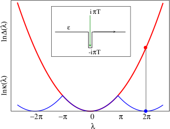
Figure 3: Analytic ${\overline{\Delta}}_{\eta\tau}(\lambda)$ vs. periodic $\kappa(\lambda)$ continuation of the functional determinant. The value of ${\overline{\Delta}}_{\eta\tau}$ at $\lambda=2\pi$ determines the free-electron GF, while $\ln\kappa(2\pi)=0$ in view of charge quantization. As an example, the equilibrium case is shown. Inset: contour of integration for the quasiclassical limit, Eq. (66), of ${\overline{\Delta}}_{\eta\tau}(\lambda)$ is deformed, since a singularity of the integrand crosses the real axis at $\lambda=\pi$.

IV Fermi Edge Singularity

A natural question to ask is whether values of $\Delta_{\eta\tau}(\lambda)$ away from $\lambda=2\pi$ are physically important. To see that this is indeed the case, consider the Fermi edge singularity (FES) problem. In this problem, an electron excited into the conduction band, leaves behind a localized hole, resulting in an $s$-wave scattering phase shift, $\delta_{0}$, of the conducting electrons Nozieres . In the mesoscopic contextMatveevLarkin , the FES manifests itself in resonant tunneling experiments Geim . On a formal level it is described by the following Hamiltonian

$$H=\sum_{k}\epsilon_{k}a_{k}^{\dagger}a_{k}+E_{0}b^{\dagger}b+\sum_{k,k^{\prime}}V_{k,k^{\prime}}a^{\dagger}_{k}a_{k^{\prime}}bb^{\dagger}\,.$$ (78)

While in the FES problem there is no interaction between electrons in the conducting band, it has many features characteristic of genuine many-body physics. Historically, the FES problem was first solved by an exact summation of an infinite diagrammatic series Nozieres . Despite the fact that conventional experimental realizations of FES are three-dimensional, the problem can be reduced (due to the local character of the interaction with the core hole) to that of one-dimensional chiral fermions. For this reason, bosonization technique can be effectively applied, leading to an alternative and very elegant solution Schotte .

Away from equilibrium, the FES has been addressed in Ref. Abanin, where the canonical (fermionic) FES theory was combined with the scattering matrix approach. Below, we apply the non-equilibrium bosonization technique to the same problem.

As mentioned above, the FES problem is effectively described by chiral 1D electrons interacting with a core hole that is instantly “switched on”. As was shown in Schotte , taking into account the core hole in the bosonization approach amounts to replacement of $e^{i{\phi}}$ by $e^{i(1-\delta_{0}/\pi){\phi}}$ in the boson representation of the fermionic operator. Using Eqs. (3), (III.4), one gets

$$G^{>}(\tau)=-\frac{i\Lambda}{2\pi v}\langle T_{K}e^{i\left(1-\frac{\delta_{0}}{\pi}\right){\phi}_{-}(0,\tau)}e^{-i\left(1-\frac{\delta_{0}}{\pi}\right){\phi}_{+}(0,0)}\rangle\,$$ (79)

and similarly for the function $G^{<}$. Within our non-equilibrium formalism, this implies a replacement $j\rightarrow(1-\delta_{0}/\pi)j$ in Eq. (58). Performing the derivation as in the free-fermion case, we thus obtain the non-equilibrium FES GF for electrons with an arbitrary distribution $n(\epsilon)$,

$$G^{\gtrless}(\tau)=\mp i\Lambda{\overline{\Delta}}_{\tau}(2\pi-2\delta_{0})/2\pi v(1\pm i\Lambda\tau)^{(1-\delta_{0}/\pi)^{2}}.$$ (80)

At equilibrium Eq. (80) can be further simplified (see Appendix A),

$$G^{\gtrless}(\tau)=\left(\frac{\pi T\tau}{\sinh\pi T\tau}\right)^{(1-\frac{\delta_{0}}{\pi})^{2}}\frac{\mp i\Lambda}{2\pi v(1\pm i\Lambda\tau)^{(1-\frac{\delta_{0}}{\pi})^{2}}}\,,$$ (81)

reproducing the known results Nozieres ; Schotte .

For a double-step distribution, Eq. (69), the long-time limit is obtained as

$$\Delta_{\tau}(2\pi-2\delta_{0})\simeq e^{-\tau/2\tau_{\phi}(2\delta_{0})}\,,$$ (82)

where the dephasing rate $\tau_{\phi}^{-1}$ is given by

$$\tau^{-1}_{\phi}(\lambda)=-\frac{eV}{2\pi}\ln\left(1-4a(1-a)\sin^{2}\frac{\lambda}{2}\right)\,.$$ (83)

In the energy representation $\tau_{\phi}^{-1}$ determines the broadening of the split FES singularities. The same result for the broadening of FES has been obtained by Abanin and Levitov in Ref. Abanin, within the fermionic framework. It is instructive to compare their result with our analysis. In the bosonization technique we have expressed the GF of the FES problem in terms of a functional determinant (80). On the other hand, within the fermionic approach Abanin the GF splits into a product of an open line $L(\tau)$ (i.e. single particle Green function of fermions in the presence of external time dependent field) and closed loop $e^{C}$ (i.e. vacuum loops of fermions in an external field),

$$G^{\gtrless}(\tau)=L^{\gtrless}(\tau)e^{C}\,,$$ (84)

with the closed-loop part given by

$$e^{C}=\Delta_{\tau}(-2\delta_{0})\,.$$ (85)

This representation of the Green function is similar to the functional bosonization approach Fogedby:76 ; LeeChen:88 ; Naon ; Yur , that employs both fermionic and bosonic variables. While functional and full bosonization approaches yield equivalent results, this equivalence is highly non-trivial. Indeed, comparing Eq. (84) with (80) and employing Eq. (85), we establish the identity

$$\mp\frac{i\Lambda}{2\pi v}\left(\frac{1\mp i\tau\Lambda}{1\pm i\Lambda\tau}\right)^{(1-\delta_{0}/\pi)^{2}}\Delta_{\tau}(2\pi-2\delta_{0})$$

$$=L^{\gtrless}(\tau){\Delta}_{\tau}(-2\delta_{0})\,$$ (86)

relating the functional determinants $\overline{\Delta}_{\tau}(2\pi-2\delta_{0})$ and $\overline{\Delta}_{\tau}(-2\delta_{0})$ through the single-particle Green function $L(\tau)$.

Since ${n}_{\eta}$ is diagonal in energy space, while ${\delta_{\eta}}$ is diagonal in time space, they do not commute, making the determinant non-trivial. It is worth noting that the functional determinants ${\overline{\Delta}}_{\tau}(\lambda)$ for $|\lambda|<\pi$ have been efficiently studied by numerical means Nazarov ; Marquardt . The identity (IV) can be useful for the numerical evaluation of ${\overline{\Delta}}_{\tau}(\lambda)$ at larger values of $\lambda$.

V interacting electrons

So far we have been dealing with non-interacting electrons. Now we focus on the main subject of this work: bosonization of interacting fermions, both for spinless and for spinful cases. We begin by showing in Sec. V.1 how the interaction can be incorporated into the non-equilibrium bosonization scheme developed above.

V.1 Keldysh action

For the problem of spinless interacting fermions the Hamiltonian reads

$$H=H_{0}+H_{\rm ee}\,,$$ (87)

where $H_{0}$ is given by Eq. (2) and

$$H_{\rm ee}=\frac{1}{2}\int dxg(x)\left(\rho_{L}(x)+\rho_{R}(x)\right)^{2}\,,$$ (88)

where $g(x)$ is a spatially dependent interaction strength. To model the coupling with non-interacting leads, we will assume that $g(x)$ is constant within the interacting part of the wire and “switches off” near the end points, $x=\pm L/2$, see Fig. 4. This way of modeling leads was introduced in Refs. Maslov, ; Ponomarenko, ; Safi, to study the conductance of a LL wire; it was also exploited in Refs. Ponomarenko96, ; Trauzettel04, to analyze the shot noise. In the Lagrangian formulation, Eqs. (87), (87) correspond to the action

$$S[\psi]=S_{0}[\psi]+S_{\rm ee}[\psi]\,,$$

$$S[\psi]=\int_{c}dt\int dx\sum_{\eta}\bigg{[}\psi^{\dagger}_{\eta}i\partial_{\eta}\psi_{\eta}-\frac{g(x)}{2}\rho^{2}(x,t)\bigg{]}\,,$$

where $\rho(x)=\rho_{R}(x)+\rho_{L}(x)$. Decoupling the interaction term via a bosonic field $\varphi$ by means of a Hubbard-Stratonovich transformation, we obtain the action

$$S[\psi,\varphi] = \int_{c}dt\int dx\bigg{[}\sum_{\eta=R,L}\psi^{\dagger}_{\eta}(i\partial_{\eta}-\varphi)\psi_{\eta}$$ (89)

$$- \frac{1}{2}\varphi g^{-1}(x)\varphi\bigg{]}\,.$$

The theory of fermions in an arbitrary field $\varphi(x,t)$ (on the Keldysh contour) can be bosonized using the results of Sec. III. Introducing, as before, notations with (without) bar for the quantum (classical) components, we obtain the action

$$S[\varphi,\bar{\varphi},\rho,\bar{\rho}]=S_{0}[\rho,\bar{\rho}]+S_{ee}[\rho,\varphi]\,,$$ (90)

where $S_{0}[\rho,\bar{\rho}]$ is the bosonized action of non-equilibrium free fermions, Eq.(31) and

$$S_{ee}[\rho,\varphi]=-\int dtdx[\varphi\bar{\rho}+\bar{\varphi}\rho+\varphi g^{-1}(x)\bar{\varphi}]\,.$$ (91)

Integrating out the auxiliary Hubbard-Stratonovich field $\varphi$, we derive a theory written solely in terms of density fields,

$$S[\rho,\bar{\rho}]=S_{0}[\rho,\bar{\rho}]-\int dtdxg(x)\rho\bar{\rho}\,.$$ (92)

Equation (92) constitutes a bosonic description for interacting electrons out of equilibrium.

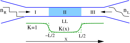
Figure 4: Schematic view of a LL conductor connected to leads with two different incoming fermionic distributions. The LL interaction parameter $K(x)$ is also shown; the dashed line corresponds to its sharp variation at the boundaries.

V.2 Tunneling spectroscopy of interacting fermions, spinless case

We are now prepared to address the problem formulated in the beginning of the paper: an interacting quantum wire out of equilibrium, Fig.4. We will first calculate the GFs at coinciding spatial points, which corresponds to tunneling spectroscopy measurements. In Sec. V.3 we will generalize this analysis to GFs at different spatial points which are, in particular, relevant to experiments on LL interferometers.

V.2.1 Tunneling into the interacting part of the wire

We consider $G_{R}^{\gtrless}(\tau)$ for the tunneling point ($x=0$) located inside the interacting part of the wire (region II in Fig. 4); generalization to tunneling into one of non-interacting leads (regions I and III in Fig. 4) is straightforward and will be presented in Sec. V.2.3.

Proceeding in the same way as for the non-interacting case, we come to a representation of the GF in the form of an integral over the density fields $\rho$ and $\bar{\rho}$, Eq. (55). The only difference as compared to the non-interacting case is that the bosonic action (92) now contains also the second term induced by the interaction. Since this term is linear in the classical component $\rho_{\eta}$, we can perform the integration over it in the same way as we did in the non-interacting case. As a result, we obtain equations satisfied by the quantum components $\bar{\rho}_{\eta}$ of the density fields,

$$\partial_{t}\bar{\rho}_{R}+\partial_{x}\left[(v+{g\over 2\pi})\bar{\rho}_{R}+\frac{g}{2\pi}\bar{\rho}_{L}\right]=j\,,$$

$$\partial_{t}\bar{\rho}_{L}-\partial_{x}\left[(v+\frac{g}{2\pi})\bar{\rho}_{L}+\frac{g}{2\pi}\bar{\rho}_{R}\right]=0\,,$$ (93)

where the source term $j(x,t)$ is defined by Eq.(57). The solution of Eq. (V.2.1) determines the phases $\delta_{\eta}(t)$ according to Eqs. (61), (63). Remarkably, Eq. (63) expresses the phase $\delta_{\eta}(t)$ affected by the electron-electron interaction, through the asymptotic behavior of $\bar{\rho}(x,t)$ in the non-interacting parts of the wire (regions I and III in Fig. 4). The phases $\delta_{\eta}(t)$ determine the GFs viafootnote_Yuval

$$G^{\gtrless}_{R}(\tau)=\mp\frac{i\Lambda}{2\pi u}\frac{\overline{\Delta}_{R}[\delta_{R}(t)]\overline{\Delta}_{L}[\delta_{L}(t)]}{(1\pm i\Lambda\tau)^{1+\gamma}},$$ (94)

where

$$\gamma=(1-K)^{2}/2K\,,$$ (95)

and

$$K=(1+g/\pi v)^{-1/2}$$ (96)

is the standard LL parameter in the interacting region.

To explicitly evaluate $\delta_{\eta}(t)$ for the structure of Fig. 4, it is convenient to rewrite Eqs. (V.2.1) as a second-order differential equation for the current

$$\bar{J}=v(\bar{\rho}_{R}-\bar{\rho}_{L}),$$ (97)

$$(\omega^{2}+\partial_{x}u^{2}(x)\partial_{x})\bar{J}(\omega,x)=0\,,\ \ x\neq 0,$$ (98)

where

$$u(x)=v(1+g(x)/\pi v)^{1/2}=\frac{v}{K(x)}\,$$ (99)

is a spatially dependent plasmon velocity. Reflection and transmission of plasmons on both boundaries is characterized by the coefficients $r_{\eta}$, $t_{\eta}$ ($r_{\eta}^{2}+t_{\eta}^{2}=1$); here the subscripts $\eta$ refer to the boundaries between regions I/II and II/III. For simplicity, we assume them to be constant over a characteristic frequency rangefootnote_tau $\omega\sim\tau^{-1}$. The scattering matrices on the left and right boundaries have the form

$$S_{L}=\left(\begin{array}[]{cc}t_{L}&-r_{L}\\ r_{L}&t_{L}\end{array}\right),\qquad S_{R}=\left(\begin{array}[]{cc}t_{R}&r_{R}\\ -r_{R}&t_{R}\end{array}\right),$$ (100)

where the first component corresponds to the left mover and the second one to the right mover.

Solution of Eq. (98) is quite straightforward. The boundary points $x=\pm L/2$ and the observation point $x=0$ divide the $x$ axis into four regions (I, II_-, II₊, and III). In each of the regions the function $\bar{J}(\omega,x)$ satisfies the homogeneous wave equation, with the velocity $v$ (in regions I and III) or $u$ (in regions II_- and II₊). The solution in each of the regions is thus a sum of two waves propagating left and right. As discussed after Eq. (58), we need an advanced solution, which imposes the condition that in the leads (regions I and III) only incoming waves are present. There remain six coefficients that are fixed by the boundary conditions at the sample/lead boundaries [see Eq. (100)] and by the matching condition at the observation point ($x=0$). The latter condition is generated by the source term in Eq. (V.2.1).

Solving Eq. (98) and using Eq. (97), we find the quantum density components $\bar{\rho}_{\eta}$. In accordance with Eq. (63) the scattering phases $\delta_{\eta}(t)$ are determined by the behavior of $\bar{\rho}_{\eta}$ in the asymptotic regions ($x<-L/2$ for $\bar{\rho}_{R}$ and $x>L/2$ for $\bar{\rho}_{L}$). We find

$$\bar{\rho}_{R}(\omega,x) = \frac{(1+K)t_{L}}{2\sqrt{2K}v}\frac{e^{ikx+i(k-\kappa)L/2}}{1-r_{R}r_{L}e^{-2i\kappa L}}\left(1-e^{i\omega\tau}\right)$$ (101)

$$\times \left(1-r_{R}re^{-i\kappa L}\right),\qquad x<-\frac{L}{2}\,;$$

$$\bar{\rho}_{L}(\omega,x) = \frac{(1+K)t_{R}}{2\sqrt{2K}v}\frac{e^{-ikx+i(k-\kappa)L/2}}{1-r_{R}r_{L}e^{-2i\kappa L}}\left(1-e^{i\omega\tau}\right)$$ (102)

$$\times \left(r+r_{L}e^{-i\kappa L}\right),\qquad x>\frac{L}{2}\,.$$

Here we use the notations $k=\omega/v$, $\kappa=\omega/u$, and $r=(1-K)/(1+K)$. Substituting this in Eq. (63), we obtain $\delta_{\eta}(t)$ in the form of a superposition of rectangular pulses,

$$\delta_{\eta}(t)=\sum_{n=0}^{\infty}\delta_{\eta,n}w_{\tau}(t,t_{n})\,,$$ (103)

where

$$t_{n}=(n+1/2-1/2K)L/u\,$$ (104)

and

$$\delta_{\eta,2m}=\pi t_{-\eta}r_{L}^{m}r_{R}^{m}(1+\eta K)/\sqrt{K}\,,$$

$$\delta_{\eta,2m+1}=-\pi t_{-\eta}r_{\eta}^{m+1}r_{-\eta}^{m}(1-\eta K)/\sqrt{K}\,.$$ (105)

For the “partial equilibrium” state (where $n_{R}(t)$ and $n_{L}(t)$ are of Fermi-Dirac form but with different temperatures and chemical potentials) the functional determinants are Gaussian functions of phases, reproducing earlier results of functional bosonization GGM_2009 . Indeed, using Eq. (176), we find

$$G^{\gtrless}_{R}(\tau) = \mp\frac{i\Lambda}{2\pi u}\frac{1}{(1\pm i\Lambda\tau)^{1+\gamma}}$$ (106)

$$\times \left(\frac{\pi T_{R}\tau}{\sinh\pi T_{R}\tau}\right)^{1+\alpha}\left(\frac{\pi T_{L}\tau}{\sinh\pi T_{L}\tau}\right)^{\beta}\,,$$

where the exponents $1+\alpha$ and $\beta$ are given by the sums

$$1+\alpha \equiv \sum_{n=0}^{\infty}\left(\frac{\delta_{R,n}}{2\pi}\right)^{2}\,,$$

$$\beta \equiv \sum_{n=0}^{\infty}\left(\frac{\delta_{L,n}}{2\pi}\right)^{2}\,.$$ (107)

Substituting here the results (V.2.1) for the phases $\delta_{\eta,n}$, we obtain

$$1+\alpha=\frac{{\cal T}_{L}}{1-{\cal R}_{L}{\cal R}_{R}}\bigg{[}1+\frac{\gamma}{2}(1+{\cal R}_{R})\bigg{]}\,,$$

$$\beta=\frac{{\cal T}_{R}}{1-{\cal R}_{L}{\cal R}_{R}}\bigg{[}{\cal R}_{L}+\frac{\gamma}{2}(1+{\cal R}_{L})\bigg{]}\,,$$ (108)

in agreement with Ref. GGM_2009, . One may check that, due to the sum rule

$$\alpha+\beta=\gamma\,,$$ (109)

at thermal equilibrium ($T_{R}=T_{L}$) the GFs $G^{\gtrless}$ are independent of plasmon transmission/reflection amplitudes.

The phases $\delta_{\eta}(t)$ are shown in Fig. 5 for two limits of adiabatic ($r_{\eta}=0$) and sharp,

$$r_{\eta}=(1-K)/(1+K)\,,$$

boundaries. Let us stress that when we speak here about sharp boundaries, we mean that the extension of the contact regions is small compared to the characteristic plasmon wave length $\sim u/\omega$. It is assumed throughout the paper that the structure is always smooth on the scale of the electron wave length, so that no electron backscattering takes place.

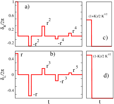
Figure 5: Phases $\delta_{\eta}(t)$ entering Eq. (94) for the GFs for sharp [a),b); $r=(1-K)/(1+K)$] and adiabatic [c),d)] boundaries.

In physical terms $\delta_{\eta}(t)$ characterizes phase fluctuations in the leads that arrive at the measurement point $x=0$ during the time interval $[0,\tau]$. These fluctuations govern the dephasing and the energy distribution of electrons encoded in the GFs $G^{\gtrless}_{\eta}(\tau)$. Up to inversion of time, one can think of $\delta_{\eta}(t)$ as describing the fractionalization of a phase pulse (electron-hole pair) injected into the wire at point $x$ during the time interval $[0,\tau]$. This is closely related to the physics of charge fractionalization discussed earlier Safi ; Oreg_Finkelstein ; safi97 ; lehur ; steinberg08 ; berg09 . At the first step, the pulse splits into two with relative amplitudes $(1+K)/2$ and $(1-K)/2$ carried by plasmons in opposite directions, cf. Refs. safi97, ; lehur, ; steinberg08, . As each of these pulses reaches the corresponding boundary, another fractionalization process takes place: a part of the pulse is transmitted into a lead, while the rest is reflected. The reflected pulse reaches the other boundary, is again fractionalized there, etc. Let us stress an important difference between boundary fractionalization of transmitted charge Safi ; berg09 and that of dipole pulses discussed here. While in the former case the boundaries can always be thought of as sharp (one is dealing with the small q limit), in the present problem the way $K(x)$ is turned on is crucially important for reflection coefficients $r_{\eta}$ at $\omega\sim\tau^{-1}$.

For $\tau\ll L/u$ the coherence of plasmon scattering may be neglected and the result splits into a product

$$\overline{\Delta}_{\eta}[\delta_{\eta}(t)]\simeq\prod_{n=0}^{\infty}\overline{\Delta}_{\eta\tau}(\delta_{\eta,n})\,,$$ (110)

with each factor representing a contribution of a single phase pulse $\delta_{\eta,n}(t)=\delta_{\eta,n}w_{\tau}(t,0)$.

We now apply our general result (94), (110) to the “full non-equilibrium” case, when $n_{\eta}(\epsilon)$ have a double step form, Eq. (69). To obtain the exact form of the Green function $G_{\eta}(\tau)$, one has to evaluate the Toeplitz determinants numerically. Here we restrict ourselves to the evaluation of the long-time asymptotics of $G_{\eta}(\tau)$ that can be found analytically employing Eq. (66) and governs the broadening of the split zero-bias-anomaly dipsGGM2008 ; GGM_2009 . We focus on the adiabatic limit when the distribution function remains unchanged and the broadening is solely due the non-equilibrium dephasing rateGGM2008 ; GGM_2009 , $1/\tau_{\phi}^{\eta}$. We obtain

$$1/\tau_{\phi}^{R}=1/\tau_{\phi}^{RR}+1/\tau_{\phi}^{RL}\,,$$ (111)

where $1/\tau_{\phi}^{\eta\eta^{\prime}}$ is the contribution to dephasing of the $\eta$ fermions governed by the distribution of the $\eta^{\prime}$ fermions. These dephasing rates are found to be

$$1/\tau_{\phi}^{R\eta}=-\frac{eV_{\eta}}{2\pi}\ln\left(1-4a_{\eta}(1-a_{\eta})\sin^{2}\frac{\pi(1+\eta K}{2\sqrt{K}}\right),$$ (112)

see Fig. 6.

Two remarkable features of this result should be pointed out. First, let us compare our results with the results of RPA approximation. Consider the weak-interaction regime, $\gamma\ll 1$. We then obtain

$$1/\tau_{\phi}^{RL}\simeq\pi\gamma eV_{L}a_{L}(1-a_{L})\,,$$ (113)

$$1/\tau_{\phi}^{RR}\simeq\pi(\gamma^{2}/8)eV_{R}a_{R}(1-a_{R})\,.$$ (114)

This should be contrasted with RPA which predicts equal $1/\tau_{\phi}^{RL}$ and $1/\tau_{\phi}^{RR}$, see Ref. GGM2008, . While $1/\tau_{\phi}^{RL}$ agrees with the RPA result, $1/\tau_{\phi}^{RR}$ is parametrically smaller (suppressed by an extra factor of $\gamma$). The reason for this failure of RPA is clear from our analysis. For a weak interaction the contributions of R and L movers to $G_{R}$ are given by the functional determinants $\Delta_{\eta\tau}(\delta_{\eta})$ with phases (for adiabatic boundaries) $\delta_{L}\simeq(1-K)\pi$ and $\delta_{R}\simeq\pi(1+K)$. While the contribution of the small phase $\delta_{L}$ is captured correctly by RPA, a small-$\delta$ expansion of $\ln\Delta_{R\tau}(\delta_{R})$ fails for large $\delta_{R}$ (apart from equilibrium and “partial equilibrium” where $\ln\Delta_{\eta\tau}(\delta)\propto\delta^{2}$.)

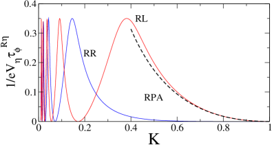
Figure 6: Dephasing rates $1/\tau_{\phi}^{RR}$ and $1/\tau_{\phi}^{RL}$ as function of LL parameter $K$ for the adiabatic case and double step distributions with $a_{R}=a_{L}=1/3$.

Another important observation is that for certain values of the interaction parameter $K$ (different for $\eta=R$ and $L$) the dephasing rates $1/\tau_{\phi}^{R\eta}$ vanish. This implies that, for these values of $K$, the GF does not decay exponentially in time, so that the power-law ZBA anomaly is not smeared. The absence of dephasing indicates that for these values of interaction the system reduces in some sense to a non-interacting model. As we are going to show, at these points the functional determinant can be calculated exactly.

V.2.2 Refermionization

The points of no-dephasing correspond to the value of the phase $\delta$ (argument of the functional determinant) equal to $\delta=2\pi n$ with an integer $n$. We will demonstrate that at these points the functional determinant $\overline{\Delta}_{\tau}(\delta)$ can be calculated exactly by “refermionization”. The case $\delta=2\pi$ corresponds to the non-interacting ($K=1$) single-particle GF and has been already analyzed in Sec. III. To study the case $\delta=4\pi$, we consider a two-fermion GF

$$G_{2}=\langle T\psi^{\dagger}(1)\psi^{\dagger}(2)\psi(3)\psi(4)\rangle\,.$$ (115)

We focus on the limit of merging points, $t_{1}=t_{2}=0$, $t_{3}=t_{4}=\tau$; $x_{1},x_{2},x_{3},x_{4}\to x$, which corresponds to simultaneous creation and annihilation of two fermions, and thus should generate $\overline{\Delta}_{\tau}(4\pi)$. For non-interacting electrons the GF $G_{2}$ can be readily calculated. Using Wick’s theorem, we find

$$G_{2}=G(3,1)G(4,2)-G(4,1)G(3,2)\,.$$ (116)

If the spatial points strictly coincide, $x_{1}=x_{2}=x_{3}=x_{4}=x$, the function $G_{2}$ vanishes. A finite result is obtained after splitting the points by distances of the order of Fermi length, $s_{i}\sim v/\Lambda$. We thus find

$$G_{2}(\tau) = \frac{1}{2}(s_{1}-s_{2})(s_{4}-s_{3})$$ (117)

$$\times (\partial_{\tilde{s}_{1}}-\partial_{\tilde{s}_{2}})^{2}G(\tau,\tilde{s}_{1})G(\tau,\tilde{s}_{2})\mid_{\tilde{s}_{1}=\tilde{s}_{2}=0}\,,$$

where $x_{i}=x+s_{i}$. In the bosonic description this corresponds to

$$G_{2}(\tau)=\left(\frac{\Lambda}{2\pi v}\right)^{2}\big{\langle}T_{K}e^{2i\phi(\tau)-2i\phi(0)}\big{\rangle}.$$ (118)

As was shown above, this correlation function can be evaluated, with the result expressed in terms of a functional determinant,

$$G_{2}(\tau)=\left(\frac{\Lambda}{2\pi v}\right)^{2}\frac{\overline{\Delta}_{\tau}(4\pi)}{(\Lambda\tau)^{4}}\,,$$ (119)

where we used $\tau\gg\Lambda^{-1}$.

Comparing Eqs. (117) and (119), we express $\overline{\Delta}_{\tau}(4\pi)$ through the free-electron GFs,

$$\overline{\Delta}_{\tau}(4\pi)=(2\pi)^{2}(v\tau)^{4}(\partial_{s_{1}}-\partial_{s_{2}})^{2}G(s_{1},\tau)G(s_{2},\tau)\,.$$ (120)

The numerical coefficient $(2\pi)^{2}$ was restored by comparison with equilibrium case. For a double-step distribution function, Eq. (69), we find from Eq. (120):

$$\!\!\!\!\!\!\!\!\overline{\Delta}_{\tau}(4\pi) = e^{2i(a-1)V\tau}\left(\frac{\pi T_{\eta}\tau}{\sinh\pi T_{\eta}\tau}\right)^{2}$$ (121)

$$\times \bigg{[}a_{\eta}(a_{\eta}-1)(V\tau)^{2}e^{iV\tau}$$

$$+ \left(a+(1-a)e^{iV\tau}\right)^{2}\left(\frac{\pi T_{\eta}\tau}{\sinh\pi T_{\eta}\tau}\right)^{2}\bigg{]}.$$

We see that $\overline{\Delta}_{\tau}(4\pi)$ shows oscillations in $\tau$. At zero temperature there is no exponential damping. The absence of damping is a manifestation of the vanishing dephasing rate, see the discussion above. Another interesting property of the result (121) is the emergence of oscillations with three frequencies: $-2aeV$, $(1-2a)eV$, and $(2-2a)eV$, implying three points of singular behavior in the energy space. Let us recall that the input double-step distribution had two such points: $-aeV$ and $(1-a)eV$. With increasing interaction strength the corresponding twofold singularity gets progressively more smeared [see Eq. (83)], but then as $\delta$ approaches $\delta=4\pi$, a threefold singularity emerges at the new positions, see Fig. 7.

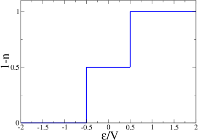
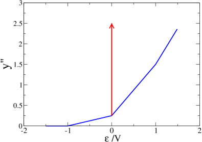
Figure 7: Refermionization at a no-dephasing point. Upper plot: double-step distribution function $1-n(\epsilon)$. Lower plot: function $y^{\prime\prime}(\epsilon/V)$, where $G^{>}_{\delta_{0}=-\pi}(\epsilon)=-i/(2v)(V/\Lambda)^{3}y(\epsilon/V)$ is the FES Green function (80) proportional to the determinant ${\overline{\Delta}}_{\tau}(4\pi)$ with the argument $\delta=4\pi$ being integer multiple of $2\pi$. The second derivative is plotted in order to emphasize singularities. The arrow at $\epsilon=0$ denotes a delta-function contribution to $y^{\prime\prime}$.

This procedure can be extended to a more general case of $\delta=2\pi n$. Indeed, the simultaneous creation and annihilation of $n$ non-interacting fermions is described by

$$G_{n}(\tau)=\langle(\psi^{\dagger}(\tau))^{n}(\psi(0))^{n}\rangle\,,$$ (122)

where we again imply a point splitting on a distance of the order of Fermi wave length, i.e. $\sim v/\Lambda$. (One can check that the relation resulting from this consideration does not depend on details of the point-splitting procedure). The function $G_{n}$ can be expressed in terms of single-particle GFs as follows:

$$G_{n}(\tau) = C_{n}s^{n(n-1)}\prod_{i\neq j}^{n}(\partial_{s_{i}}-\partial_{s_{j}})G(s_{1},\tau)$$ (123)

$$\times G(s_{2},\tau)\dots G(s_{n},\tau)\mid_{s_{i}=0}\,.$$

Here $C_{n}$ are numerical coefficients of the order of unity. On the other hand, in the bosonic framework we have

$$G_{n}(\tau)=\left(\frac{\Lambda}{2\pi v}\right)^{n}\frac{\overline{\Delta}_{\tau}(2\pi n)}{(\Lambda\tau)^{n^{2}}}\,.$$ (124)

Demanding the equivalence of Eqs. (123) and (124), we establish the identity

$$\overline{\Delta}_{\tau}(2\pi n) = C_{n}(v\tau)^{n^{2}}\prod_{i\neq j}^{n}(\partial_{s_{i}}-\partial_{s_{j}})$$ (125)

$$\times G(s_{1},\tau)\dots G(s_{n},\tau))\mid_{s=0}\,,$$

expressing the functional determinant $\overline{\Delta}_{\tau}(\delta)$ through free fermionic GFs $G(\tau)$ for $\delta=2\pi n$. The numerical coefficients $C_{n}$ can be restored by comparison with the known result for $\overline{\Delta}_{\tau}(2\pi n)$ at equilibrium. The explicit form of $\overline{\Delta}_{\tau}(\delta=2\pi n)$ can be readily found by substituting in Eq. (125) an explicit expression for the GF for a given distribution function.

V.2.3 Tunneling into non-interacting regions

Next we discuss the tunneling spectroscopy for the non-interacting parts of the wire. Let us focus on the right-moving electrons; the analysis of left-moving ones can be done in the same way. For $x_{1},x_{2}<-L/2$ (region I in Fig. 4) the GF is the one of free fermions, as the right-moving particles emerging from the left reservoir are not yet aware of the interacting region they are about to enter. The situation is less trivial for $x_{1},x_{2}>L/2$ (region III). Indeed, while the strength of the interaction in this region is zero, right-moving electrons there have passed through the interacting part of the wire, which modifies their Green function. We will show below that the GFs $G^{\gtrless}_{R}(x_{1},t_{1};x_{2},t_{2})$ in the non-interacting region satisfy Galilean invariance: they depend on $(x_{1}-vt_{1})-(x_{2}-vt_{2})$ only. For this reason, it is sufficient to consider $x_{1}=x_{2}$ to obtain the full information about the GF.

The evaluation of the GF is performed in the same way as in the interacting region, yielding the result (94). The phases $\delta_{\eta}(t)$ are now given by

$$\delta_{R}(t) = \sum_{n=0}^{\infty}\delta_{R,n}w_{\tau}(t,x_{1}/v+2t_{n})\,,$$ (126)

$$\delta_{L}(t) = 2\pi r_{R}w_{\tau}\left(t,\frac{x_{1}-L}{v}\right)$$ (127)

$$+ \sum_{n=0}^{\infty}\delta_{L,n}w_{\tau}\left(t,\frac{x_{1}}{v}+\frac{L}{u}+2t_{n}\right)\,,$$

with the following amplitudes of rectangular pulses:

$$\delta_{R,n} = 2\pi t_{L}t_{R}(r_{L}r_{R})^{n}\,,$$

$$\delta_{L,n} = -2\pi(r_{L}r_{R})^{n}r_{L}t_{R}\,.$$ (128)

In the case of smooth boundaries only one pulse is created, $\delta_{R,0}=2\pi$, reproducing the free fermion GF. Thus, in the adiabatic case, the interaction has no influence on GFs in the non-interacting parts of the wire, as expected. If the transition between non-interacting and interacting parts of the wire is not smooth, plasmon scattering takes place. This process leads to a redistribution of electrons over energies GGM_2009 and thus affects GFs in the non-interacting region.

V.3 Green functions at different points and Aharonov-Bohm interferometry

So far we have discussed GFs at coinciding spatial points, having in mind tunneling spectroscopy experiments. We now consider GFs at different spatial coordinates. Such GFs are relevant to various physical quantities, in particular, in the context of Aharonov-Bohm interferometry. The similar problem in the context of chiral edge state has been considered in Refs. Chalker, ; Sukhorukov, . Let us consider a four-terminal setup formed by two quantum wires coupled by tunneling at two points, as schematically shown in Fig. 8. Each one of the quantum wires is assumed to be a LL conductor connected to two non-interacting electrodes with arbitrary (in general, non-equilibrium) distribution functions, as shown in Fig.4. We are interested in the Aharonov-Bohm effect, i.e. the dependence on the magnetic flux $\Phi$ of the electric current flowing from wire 1 into wire 2. Consider the situation where the tunnel coupling between the wires 1 and 2 is weak. We also assume that both arms of the AB-interferometer have equal length $d$ and tunneling occurs at points located inside the interacting part of the wire. The flux dependent part of the electric current is given by

$$I_{\phi} = |t_{12}|^{2}\int_{-\infty}^{\infty}dte^{-i\phi}[G_{2}^{<}(d,t)G^{>}_{1}(-d,-t)$$ (129)

$$- G_{2}^{>}(d,t)G_{1}^{<}(-d,-t)]+{\rm h.c.}\,,$$

where the subscripts 1 and 2 label the wire and $t_{12}$ is the tunneling matrix element between the wires. Separating the GF into left and right moving part, one gets

$$I_{\phi} = |t_{12}|^{2}\sum_{\eta}\int_{-\infty}^{\infty}dte^{-i\phi}[G_{2,\eta}^{<}(d,t)G^{>}_{1,\eta}(-d,-t)$$ (130)

$$- G_{2,\eta}^{>}(d,t)G_{1,\eta}^{<}(-d,-t)]+{\rm h.c.}\,$$

where we have neglected terms that oscillate fast with the interferometer size $d$.

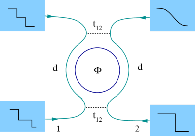
Figure 8: Aharonov-Bohm setup in a four terminal geometry, with tunnel coupling (dashed lines) at two points. Both interferometer arms have length d.

To analyze the GF $G_{\eta}^{\gtrless}(x_{1},x_{2},\tau)$ between two different points of a wire, we proceed in the same way as in the case $x_{1}=x_{2}$ above. Integration over the classical component of the density field leads to equations of motion for its quantum component (we choose $\eta=R$ for definiteness),

$$(-i\omega+v\partial_{x})\bar{\rho}_{R,\omega}+\partial_{x}\left(\frac{g}{2\pi}\bar{\rho}_{\omega}\right)=j(\omega,x;x_{1},x_{2},\tau)\,,$$

$$(i\omega+v\partial_{x})\bar{\rho}_{L,\omega}+\partial_{x}\left(\frac{g}{2\pi}\bar{\rho}_{\omega}\right)=0\,,$$ (131)

where we have used the $(\omega,x)$ representation; $\bar{\rho}_{\omega}=\bar{\rho}_{R,\omega}+\bar{\rho}_{L,\omega}$. Equations (V.3) differ from the earlier Eq. (V.2.1) only by the source term, which now reads

$$j(\omega,x;x_{1},x_{2},\tau)=\frac{1}{\sqrt{2}}\bigg{[}\delta(x-x_{1})e^{i\omega\tau}-\delta(x-x_{2})\bigg{]}\,.$$ (132)

Solving Eq. (V.3), we find for $x<-L/2$

$$\bar{\rho}_{R}(\omega,x) = \frac{(1+K)t_{L}}{2\sqrt{2K}v}\frac{e^{ikx+i(k-\kappa)L/2}}{1-e^{-2i\kappa L}r_{R}r_{L}}$$ (133)

$$\times \bigg{[}e^{-i\kappa x_{2}}-e^{i(\omega\tau-\kappa x_{1})}-r_{R}re^{i(x_{2}-L)\kappa}$$

$$+ r_{R}re^{i\omega\tau+i(x_{1}-L)\kappa}\bigg{]}\,.$$

Similarly, we find for $x>L/2$

$$\bar{\rho}_{L}(\omega,x)=\frac{(1+K)t_{R}}{2\sqrt{2K}v}\frac{e^{-ikx+i(k-\kappa)L/2}}{1-e^{-2i\kappa L}r_{R}r_{L}}$$

$$\bigg{[}re^{i\kappa x_{2}}-re^{i(\omega\tau+\kappa x_{1})}$$

$$+r_{L}e^{i\omega\tau-(x_{1}+L)\kappa}-r_{L}e^{-i(x_{2}+L)\kappa}\bigg{]}\,.$$ (134)

Employing Eqs. (63), (133) and (V.3), we obtain the following result for the GF:

$$G^{\gtrless}_{R}(x_{1},x_{2},\tau)=-\frac{1}{2\pi u(\pm i\Lambda)^{\gamma}}$$

$$\times\frac{\overline{\Delta}_{R}[\delta_{R}(t)]\overline{\Delta}_{L}[\delta_{L}(t)]}{(\tau-\frac{x_{1}-x_{2}}{u}\mp\frac{i}{\Lambda})^{1+\alpha}(\tau+\frac{x_{1}-x_{2}}{u}\mp\frac{i}{\Lambda})^{\beta}}\,.$$ (135)

It is interesting to note that for spatially separated points the scaling of GF with time (and consequently with energy) is affected by plasmon scattering at the boundaries between wire and the leads. Surprisingly, even at equilibrium the GF inside interacting region is affected by the way interaction is turned on. For coinciding spatial points the universal LL exponents, characteristic of an infinite wire, are restored due to the sum rule (109).

In the long wire limit the functional determinant splits, as before, into a product

$$\overline{\Delta}_{R}[\delta_{R}(t)]\simeq\prod_{n=0}^{\infty}\overline{\Delta}_{R,\tau-\frac{x_{1}-x_{2}}{u}}(\delta_{R,2n})\overline{\Delta}_{R,\tau+\frac{x_{1}-x_{2}}{u}}(\delta_{R,2n+1})\,.$$ (136)

Here $\delta_{\eta,n}$ are given by Eq. (V.2.1). The calculation of $\overline{\Delta}_{L}$ is performed in a similar way, yielding

$$\overline{\Delta}_{L}[\delta_{L}(t)]\simeq\prod_{n=0}^{\infty}\overline{\Delta}_{L,\tau+\frac{x_{1}-x_{2}}{u}}(\delta_{L,2n})\overline{\Delta}_{L,\tau-\frac{x_{1}-x_{2}}{u}}(\delta_{L,2n+1})\,.$$ (137)

We see that in the case of a GF at different spatial points the time argument of $\overline{\Delta}_{\eta,\tau}(\delta_{\eta})$ (determining the duration of the pulses) is replaced as compared to the case of $x_{1}=x_{2}$ by

$$\tau\rightarrow\tau\mp\eta\frac{x_{1}-x_{2}}{u}\,,$$ (138)

with the $-$ ($+$) sign corresponding to even (respectively, odd) pulses. It is easy to understand the reason for these alternating signs. The even pulses are those that experience an even number of reflections, thus preserving their chirality, while the odd pulses experience an odd number of reflections and thus invert their chirality. We note that in the case when both points are located in one of the non-interacting regions ($x_{1},x_{2}>L/2$ or $x_{1},x_{2}<-L/2$), the same consideration leads to an analogous replacement of the time argument but with the bare velocity $v$,

$$\tau\rightarrow\tau-\frac{x_{1}-x_{2}}{v}$$ (139)

in the phases $\delta_{\eta}(t)$, Eqs. (126) and (127), entering $\overline{\Delta}_{\eta,\tau}(\delta_{\eta})$ and, correspondingly, in GFs. Since there is no fractionalization at the tunneling processes into a non-interacting region, only half of the pulses survives and no sign alternation arises.

Of particular interest is the value of GF at the interaction-renormalized “light cone”, $x_{1}-x_{2}=\pm ut$. The value of the GF at these points determines the integral for the interference current in Eq. (130), see also Refs. lehur, ; GMP, . Let us consider for simplicity the case of adiabatic barrier ($r_{L}=r_{R}=0$) when each of the products (136), (137) reduces to the first factor. Compared to the limit of coinciding spatial points, the duration of pulse in the functional determinant has changed. The contribution associated with ($x_{1}-x_{2}=\eta ut$) leads to a doubling of pulse duration in $\overline{\Delta}_{-\eta}$ , while $\overline{\Delta}_{\eta}$ has disappeared altogether. As we see now, the dephasing rate governing the exponential damping of the GF $G_{\eta}^{\gtrless}$ at $x_{1}-x_{2}=\eta^{\prime}u\tau$ is

$$1/\tau_{\phi(\eta^{\prime})}^{AB;\eta}=2/\tau_{\phi}^{\eta,-\eta^{\prime}}\,,$$ (140)

where $1/\tau_{\phi}^{\eta\eta^{\prime}}$ are the partial dephasing rates for the tunneling spectroscopy problem (coinciding spatial points), as introduced in Sec. V.2.1. The dephasing rates (140) manifest themselves in the interferometry measurements by inducing an exponential damping of the corresponding contributions to the Aharonov-Bohm oscillations (thus the superscript “AB”). In the limit of large interferometer size $d$, the contribution with the lowest dephasing rate will dominate,

$$1/\tau_{\phi}^{AB}=\min_{\eta,\eta^{\prime}=R,L}2/\tau_{\phi}^{\eta\eta^{\prime}}\,.$$ (141)

For double step distributions, the dephasing rates (140) are given (up to a factor of 2) by Eq. (112). With increasing interaction the dephasing rate $1/\tau_{\phi}^{AB}$ begins to oscillate as a function of interaction parameter $K$, as illustrated (for the case of adiabatic contacts with leads) in Fig. 6. This leads to a remarkable prediction: the visibility of Aharonov-Bohm oscillations should be a strongly oscillating function of the interaction strength.

V.4 Spinful Luttinger liquid

We now consider the problem of tunneling spectroscopy for spinful electrons. The analysis is a straightforward extension of the spinless case, analyzed in Sec. V.2. We begin with a fermionic Hamiltonian, which, in the spinful case, is given by

$$H = H_{0}+H_{\rm ee}\,,$$ (142)

$$H_{0} = -iv\sum_{\sigma}\left(\psi_{R,\sigma}^{\dagger}\partial_{x}\psi_{R,\sigma}-\psi^{\dagger}_{L,\sigma}\partial_{x}\psi_{L,\sigma}\right)\,,$$ (143)

$$H_{ee} = \frac{1}{2}\sum_{\eta,\eta^{\prime};\sigma,\sigma^{\prime}}\int dxg(x)\rho_{\eta,\sigma}\rho_{\eta^{\prime},\sigma^{\prime}}\,.$$ (144)

where the index $\sigma=\uparrow,\downarrow$ labels the spin projection. We now switch to a Lagrangian description. To construct the free part of the action on the Keldysh contour we repeat the steps described in detail in Sec. III and find

$$S_{0}=\sum_{\eta=R,L;\sigma=\uparrow,\downarrow}\bar{\rho}_{\eta,\sigma}\Pi^{a^{-1}}_{\eta}\rho_{\eta,\sigma}-i\ln Z[\bar{\chi}_{\eta,\sigma}]\,,$$ (145)

where

$$\bar{\chi}_{\eta,\sigma}=\Pi_{\eta}^{a^{-1}}\bar{\rho}_{\eta,\sigma}\,.$$ (146)

The interacting part of the action reads

$$S_{ee}=-\sum_{\eta,\eta^{\prime},\sigma,\sigma^{\prime}}\int dxg(x)\rho_{\eta,\sigma}\bar{\rho}_{\eta^{\prime},\sigma^{\prime}}\,.$$ (147)

To describe the tunneling spectroscopy measurements, we need to find the single-particle GFs

$$G^{<}_{0,\eta,\sigma}(x,t)=i\langle\psi^{\dagger}_{\eta,\sigma}(0,0)\psi_{\eta,\sigma}(x,t)\rangle\,,$$

$$G^{>}_{0,\eta,\sigma}(x,t)=-i\langle\psi_{\eta,\sigma}(x,t)\psi^{\dagger}_{\eta,\sigma}(0,0)\rangle\,.$$ (148)

The fermionic operators are expressed in terms of bosonic fields (which now also carry the spin label) in the usual way,

$${\psi}_{\eta,\sigma}(x)\simeq\left(\frac{\Lambda}{2\pi v}\right)^{1/2}e^{i\eta p_{F}x}e^{i{\phi}_{\eta,\sigma}(x)}\,.$$ (149)

Substituting Eq. (149) into Eq. (V.4), representing the GF as a bosonic functional integral with the action $S_{0}+S_{ee}$, and performing the integration over the classical component of the density field, we find the equation of motion satisfied by the quantum components of the field,

$$(\partial_{t}+v\partial_{x})\bar{\rho}_{R}+\partial_{x}\frac{g}{2\pi}(\bar{\rho}_{R}+\bar{\rho}_{L})=j(x,t)\,,$$

$$(-\partial_{t}+v\partial_{x})\bar{\rho}_{L}+\partial_{x}\frac{g}{2\pi}\left(\bar{\rho}_{R}+\bar{\rho}_{L}\right)=0\,,$$ (150)

and

$$(\partial_{t}+v\partial_{x})\bar{s}_{R}=j(x,t)\,,$$

$$(-\partial_{t}+v\partial_{x})\bar{s}_{L}=0\,.$$ (151)

Here we have passed to new variables that describe the spin and charge sectors of excitations,

$$\bar{\rho}_{R}=\bar{\rho}_{R,\uparrow}+\bar{\rho}_{R,\downarrow}\,,\ \ \bar{\rho}_{L}=\bar{\rho}_{L,\uparrow}+\bar{\rho}_{L,\downarrow}$$

$$\bar{s}_{R}=\bar{\rho}_{R,\uparrow}-\bar{\rho}_{R,\downarrow}\,,\ \ \bar{s}_{L}=\bar{\rho}_{L,\uparrow}-\bar{\rho}_{L,\downarrow}\,.$$ (152)

As one sees, the equations for the charge and spin degrees of freedom are decoupled, which is a manifestation of spin-charge separation. The spin-density component obeys the same equation as the density of free fermions, Eq. (58). Therefore, the spin sector is characterized by a LL parameter $K_{s}=1$. As follows from Eq.(V.4), the spin component $s_{\eta}$ propagates through the wire without any reflection.

To find the charge component, we define the charge density current

$$\bar{J}=v(\bar{\rho}_{R}-\bar{\rho}_{L})\,.$$ (153)

In terms of $\bar{J}$, equations (V.4) are reduced to a second order differential equation,

$$(\omega^{2}+\partial_{x}u^{2}_{c}\partial_{x})\bar{J}=0\qquad{\rm for}\,\,x\neq 0,$$ (154)

where

$$u_{c}^{2}(x) = v^{2}/K^{2}_{c}(x)\,,$$

$$K_{c} = \left(1+\frac{2g}{\pi v}\right)^{-1/2}.$$ (155)

Equation (154) coincides with Eq. (98) up to a different definition of the LL parameter. The interaction parameter $\gamma=(1-K_{c})^{2}/2K_{c}$ and the transmission and reflection amplitudes are determined as for spinless fermions, with the replacement $K\rightarrow K_{c}$.

The resulting expression for the Green function of spinful fermions within the non-equilibrium bosonization approach reads

$$G^{\gtrless}_{R,\uparrow}(\tau)=\mp\frac{i\Lambda}{2\pi\sqrt{uv}}\frac{\prod_{\eta,\sigma}\overline{\Delta}_{\eta,\sigma}[\delta_{\eta,\sigma}(t)]}{(1\pm i\Lambda\tau)^{1+\gamma/2}}.$$ (156)

Here we have assumed for generality that distribution functions of spin-up and spin-down particles may be different. Therefore, the distribution function is labeled by two indices (chirality and spin projection); these indices are inherited by the functional determinant. The time-dependent phases of the spinful fermions $\delta_{\eta,\sigma}(t)$ are expressed in terms of the scattering phases $\delta_{\eta}(t)$ of spinless fermions, Eq. (103), in the following way:

$$\delta_{L,\uparrow}(t)=\delta_{L,\downarrow}(t)=\frac{1}{2}\delta_{L}(t)\,,$$ (157)

$$\delta_{R,\uparrow}(t)=\frac{1}{2}\left(\delta_{R}(t)+\delta^{0}_{R}(t)\right)\,,$$ (158)

$$\delta_{R,\downarrow}(t)=\frac{1}{2}\left(\delta_{R}(t)-\delta^{0}_{R}(t)\right)\,,$$ (159)

where $\delta^{0}_{R}(t)$ corresponds to non-interacting fermions and consists of a single pulse with an amplitude $2\pi$, $\delta^{0}_{R}(t)=2\pi w_{\tau}(t,0)$.

We conclude that the inclusion of spin changes the scattering phases in an essential way. This is most importantly seen when considering the first pulse propagating to the right. Let us assume that there is no reflection at the boundaries with non-interacting leads. The corresponding scattering phases are each a superposition of the spin and charge modes, see Eqs. (158), (159). Since the velocities of these modes are different ($v$ and $u$, respectively), then for sufficiently long wires, $L(v^{-1}-u^{-1})/\tau\gg 1$, the first pulse splits into a charge and a spin parts. For a short wire, the spin pulse and the first charge pulse overlap. In this case one has to deal with the general formula (156) and with time-dependent phase containing both, spin and, charge contributions. Hence, if the wire is sufficiently short (or, in other words, for a given length of the wire the interaction is sufficiently weak) the spin-charge separation does not have enough time to develop. For sufficiently long wires, spin-charge separation does take place, in which case the respective determinants can be written as products of spin and charge contributions. This decomposition is not valid for short wires (or, for a given length of the wire, for sufficiently weak interaction). Note that at equilibrium there is significant simplification. The GFs depend only on the sum of the scattering phases squared, see Eq. (106). Due to the sum rule (109) this combination remains unchanged, regardless of whether spin and charge pulses overlap or not. Thus, at equilibrium one can always think about these two modes separately and additively. Out of equilibrium, the dependence of the GF on scattering phases is more subtle, and the results for overlapping and separated pulses are different. Therefore, the spin-charge separation occurs in this case only for sufficiently long wires. Focusing on this regime, we find

$$\overline{\Delta}_{R,\uparrow}[\delta_{R,\uparrow}] = \overline{\Delta}_{R,\tau,\uparrow}(\pi)\prod_{n=0}^{\infty}\overline{\Delta}_{R,\tau,\uparrow}\bigg{(}\frac{\delta_{R,n}}{2}\bigg{)},$$ (160)

$$\overline{\Delta}_{R,\downarrow}[\delta_{R,\downarrow}] = \overline{\Delta}_{R,\tau,\downarrow}(-\pi)\prod_{n=0}^{\infty}\overline{\Delta}_{R,\tau,\downarrow}\bigg{(}\frac{\delta_{R,n}}{2}\bigg{)},$$ (161)

$$\overline{\Delta}_{L,\sigma}[\delta_{L,\sigma}] = \prod_{n=0}^{\infty}\overline{\Delta}_{L,\tau,\sigma}\bigg{(}\frac{\delta_{L,n}}{2}\bigg{)}.$$ (162)

The first factor in each of Eqs. (160) and (161) originate from the spin mode yielding the phase $\pi$, i.e. a half of the free-fermion phase value. The scattering phases of other pulses (originating from the charge mode) have a half of their values for spinless electrons.

Let us analyze this result. Consider the case of smooth (adiabatic) contacts with leads, so that only one pulse passes in each direction (all $\delta_{\eta,n}$ with $n\geq 1$ are zero). For the case of partial equilibrium, the determinants can be evaluated explicitly, yielding

$$\prod_{\sigma=\uparrow,\downarrow}\overline{\Delta}_{R,\sigma}[\delta_{R,\sigma}(t)]=\left(\frac{\pi T_{R}\tau}{\sinh\pi T_{R}\tau}\right)^{1+\alpha/2}\,,$$

$$\prod_{\sigma=\uparrow,\downarrow}\overline{\Delta}_{L,\sigma}[\delta_{L,\sigma}(t)]=\left(\frac{\pi T_{L}\tau}{\sinh\pi T_{L}\tau}\right)^{\beta/2}\,,$$ (163)

where $\alpha,\beta$ are given by Eq. (V.2.1). For a double-step distribution function, a semiclassical limit of the determinants (160), (161), (162) can be readily evaluated. In the large-time limit the behavior of the r.h.s. of Eqs. (160), (161), (162) is exponential, yielding the partial decay rates

$$\Gamma^{RR} = -\frac{eV}{\pi}\bigg{[}\ln\left(1-4a(1-a)\right)$$

$$+ \sum_{n=0}^{\infty}\ln\left(1-4a(1-a)\sin^{2}\frac{\delta_{R,n}}{4}\right)\bigg{]}\,,$$

$$\Gamma^{RL} = -\frac{eV}{\pi}\sum_{n=0}^{\infty}\ln\left(1-4a(1-a)\sin^{2}\frac{\delta_{L,n}}{4}\right)\bigg{]}\,,$$

and the total rate $\Gamma^{R}=\Gamma^{RR}+\Gamma^{RL}$. Let us stress an important difference with the spinless case. There, for smooth boundaries, the distribution function was not affected, and the decay rate (inducing the smearing of singularities in tunneling spectroscopy) was solely due to dephasing. In the spinful case the situation is different: independently of the shape of the boundary the spin-charge separation affects the distribution function of electrons. Indeed, imagine that we perform the tunneling spectroscopy of right-movers in the right lead (non-interacting region III of Fig. 4) for the case of adiabatic boundaries. Then the phases are $\delta_{L,n}=\delta_{R,n\neq 0}=0$ and $\delta_{R,0}=2\pi$. In the spinless case this implied that the distribution function remained unchanged. This is not so in the spinful situation, however: according to Eqs. (160), (161) we get now a product of four determinants with arguments $\pm\pi$,

$$[\overline{\Delta}_{R,\tau,\uparrow}(\pi)]^{2}\overline{\Delta}_{R,\tau,\downarrow}(-\pi)\overline{\Delta}_{R,\tau,\downarrow}(\pi)\,,$$ (165)

implying that the distribution function has changed. This effect remains finite even in the limit of vanishing interaction ($K\to 1$) as long as the long-wire condition, $LT(u^{-1}-v^{-1})\gg 1$, is satisfied. Returning to the spectroscopy of the interacting region, we conclude that both effects—dephasing and change of the distribution function—are necessarily present in the spinful LL case and cannot be easily “disentangled”. The decay rates $\Gamma$ presented in Eq. (LABEL:Gamma-spinful) and in Fig. 9 yield the combined effect of interaction on the GF $G^{\gtrless}_{R}(\tau)$ and determine the smearing of tunneling spectroscopy singularities in the energy space.

Figure 9: Decay rates $\Gamma^{RR}$ and $\Gamma^{RL}$ (governing smearing of tunneling spectroscopy singularities) as functions of LL parameter $K_{c}$ for spinful fermions. The adiabatic coupling to leads and the double-step distributions with $a_{R}=a_{L}=1/3$ are assumed.

Finally we discuss the extension of Eq. (156) to the case of GFs at different points. In this case we find

$$G^{\gtrless}_{R,\uparrow}(x_{1},x_{2},\tau)=\mp\frac{i\Lambda}{2\pi\sqrt{uv}}$$

$$\times\overline{\Delta}_{R,\uparrow,\tau-\frac{x}{v}}(\pi)\overline{\Delta}_{R,\downarrow,\tau-\frac{x}{v}}(-\pi)$$

$$\times\frac{\prod_{n=0}^{\infty}\overline{\Delta}_{R,\uparrow,\tau_{n}^{R}}\left(\frac{\delta_{R,n}}{2}\right)\prod_{n=0}^{\infty}\overline{\Delta}_{R,\downarrow,\tau_{n}^{R}}\left(\frac{\delta_{R,n}}{2}\right)}{\left(1\pm i\Lambda\left(\tau-\frac{x}{v}\right)\right)^{1/2}\left(1\pm i\Lambda\left(\tau-\frac{x}{u}\right)\right)^{1/2}}$$

$$\times\frac{\prod_{n=0}^{\infty}\overline{\Delta}_{L,\uparrow,\tau_{n}^{L}}\left(\frac{\delta_{L,n}}{2}\right)\prod_{n=0}^{\infty}\overline{\Delta}_{L,\downarrow,\tau_{n}^{L}}\left(\frac{\delta_{L,n}}{2}\right)}{\left(1\pm i\Lambda\left(\tau-\frac{x}{u}\right)\right)^{\alpha/2}\left(1\pm i\Lambda\left(\tau+\frac{x}{u}\right)\right)^{\beta/2}}\,,$$

(166)

where $x=x_{1}-x_{2}$ and $\tau_{n}^{\eta}=\tau+\eta(-1)^{n+1}x/u$. As for the spinless case, Eq. (V.3), the scaling of GFs with spatially separated points is affected by plasmon scattering at the boundaries between the interacting regions and the leads even at equilibrium.

Before concluding this section, we point out a connection between the spinful LL and the problem of the integer quantum Hall edge with two edge channels (corresponding to two Landau levels below the Fermi energy in the bulk). Non-equilibrium properties and quantum coherence of such a system are currently attracting large interest, in particular, in connection with experiments on quantum Hall Mach-Zehnder interferometers MachZehnder . In the quantum Hall setup the edge channel index plays a role of spin. The main difference is that, under conventional circumstances (if one does not make special efforts to couple counterpropagating edge modes), the quantum Hall system is chiral: there are, say, only right-moving modes and no left-movers. This leads to a number of essential simplifications: (i) the tunneling density of states becomes trivial (no ZBA); (ii) the charge fractionalization is absent (since plasmons can move only in one direction). What remains is the charge-spin separation. This implies that following simplifications with functional determinants (160), (161), (162) the product of which determined the tunneling spectroscopy Green function $G^{\gtrless}_{R,\uparrow}(\tau)$ within our analysis. First, the left-mover determinants (162) are now absent. Second, out of the set of phases $\delta_{R,n}$ only the $n=0$ phase remains, being equal to its free-fermion value, $\delta_{R,0}=2\pi$. Therefore, the product of determinants takes the form (165) (that has appeared above in the context of a GF in the non-interacting region of a non-chiral spinful wire with adiabatic contacts). The analogous statement holds for the Green function with different spatial points, Eq. (166). Specifically, for the case of the two-channel chiral setup (relevant in the quantum Hall Mach-Zehnder interferometry context MachZehnder ) the last fraction (having L determinants in the numerator) in Eq. (166) disappears, while in the preceding-to-it fraction one should keep only $n=0$ factor and set $\delta_{R,0}=2\pi$. An equivalent result was obtained by a different method in the recent work Sukhorukov .

VI Summary

Let us summarize the main results of this work, following the flow of our presentation in the paper.

1. We have developed a nonequilibrium bosonization approach and derived a bosonic theory describing the LL of interacting 1D electrons out of equilibrium. The theory is characterized by an action depending on density fields defined on the Keldysh time contour. In contrast to the equilibrium case, this theory is not Gaussian, which is a manifestation of the fact that the density matrix is non-diagonal in the bosonic Fock space. We have used this theory to calculate the electronic GFs governing various observables.

2. We have first calculated the GF of non-interacting fermions from our non-equlibrium bosonization approach. The GF is expressed in terms of a functional determinant of the Fredholm (more specifically, Toeplitz) type similar to those that have earlier appeared in the context of counting statistics. The key difference is that in the case of counting statistics the determinant is non-analytic and $2\pi$-periodic in the counting field (which reflects charge quantization), while in our theory the determinant should be understood as an analytically continued function. We have found that the free-fermion GF is described by the determinant exactly at the point $2\pi$, which is related to the fact that in the bosonic theory a fermion is represented by a $2\pi$-soliton.

3. We have next generalized the GF calculation to the problem of non-equilibrium Fermi edge singularity describing excitation of an electron into the conduction band within the process of photon absorption, accompanied by creation of a core hole. The result is obtained in terms of the same functional determinant as in the free-fermion case but the argument is now shifted from $2\pi$ by twice the scattering phase on the core hole.

4. We have then applied our formalism to the problem of interacting 1D fermions. We have considered a model of a LL wire coupled to non-interacting 1D leads, with the interaction strength “turned on” in specified fashion at the boundary between the wire and each of the leads. We have shown that the electron GFs—which describe tunneling spectroscopy measurements—are again expressed in terms of Fredholm determinants. The phases $\delta_{\eta}(t)$ entering the expressions for the corresponding operators have a physical interpretation in terms of fractionalization processes taking place during the tunneling event, near the boundaries. If the characteristic energy scales for the tunneling spectroscopy are large compared to the inverse flight time through the LL wire (Thouless energy)—which means that we are considering the truly 1D (rather than 0D) regime—the functions $\delta_{\eta}(t)$ represent a sequence of rectangular pulses separated by large intervals. As a result, the Fredholm determinant splits into a product of Toeplitz determinants of the same type as in the cases of non-interacting fermions and the Fermi edge singularity.

5. We have analyzed the long-time asymptotics of the determinant which yields the dephasing rate controlling the smearing of LL tunneling singularities (zero-bias anomaly). The dephasing rate for the GF of electrons with $\eta$ ($\pm 1$) chirality is a sum of two terms $\sum_{\eta^{\prime}=\pm 1}1/\tau_{\phi}^{\eta\eta^{\prime}}$ originating from functional determinants which depend on the distribution function of left- ($\eta^{\prime}=-1$) and right- ($\eta^{\prime}=1$) moving electrons, respectively. For the case of double-step distributions, there are two important findings:

   (i) At weak interaction, comparing our exact results with those of the RPA, we find that while $1/\tau_{\phi}^{\eta,-\eta}$ is correctly obtained (to leading order) within RPA, the RPA result for $1/\tau_{\phi}^{\eta,\eta}$ is parametrically wrong. This demonstrates that even for a weak interaction a naive perturbative expansion (leading to RPA) may be parametrically incorrect in LL out of equilibrium.

   (ii) Both $1/\tau_{\phi}^{\eta,\pm\eta}$ are oscillatory functions of the interaction strength (or, equivalently, LL parameter $K$). Furthermore, each of them vanishes at certain values of $K$. At these values the “counting phase” for the corresponding determinant becomes an integer multiple of $2\pi$. We have calculated the determinants at these no-dephasing points by a refermionization procedure.

6. We have generalized the above results to the case of a GF with two different spatial arguments. When considering the value of the GF $G_{\eta}$ at its main peak, $x_{1}-x_{2}=\eta ut$, the dephasing rate is $2/\tau_{\phi}^{\eta,-\eta}$, while $1/\tau_{\phi}^{\eta,\eta}$ does not contribute (and thus RPA is restored for weak interaction). The situation is reversed for the value of the $G_{\eta}$ at the other peak, $x_{1}-x_{2}=-\eta ut$, where the dephasing rate is $2/\tau_{\phi}^{\eta,\eta}$. Such GFs (with $x_{1}-x_{2}=\pm\eta ut$) enter the expression for the interference contribution to current in an Aharonov-Bohm interferometer formed by two LLs coupled by tunneling at two points. Our results imply that the dephasing rate in such a non-equilibrium LL interferometer (and thus the visibility of Aharonov-Bohm oscillations) is an oscillatory function of the interaction strength.

7. We have also considered the case of a spinful LL. The general structure of the results for the GFs is similar, with the key difference being that now we encounter products of determinants with phase arguments corresponding to the spin and charge sectors. This is a manifestation of the spin-charge separation. One important consequence is that the temporal decay rate of the Green function (and thus the smearing of singularities in the tunneling spectroscopy) remains finite in the limit of vanishing interaction strength, assuming the limit of the large system size is taken first. With increasing interaction strength, the dephasing rate oscillates, similarly to the case of spinless fermions.

The non-equilibrium bosonization formalism developed in this work has a variety of further applications. They include, in particular, counting statistics of charge transfer in an interacting 1D system away from equilibrium, analysis of many-body entanglement, quantum wires with several channels, etc. Generalizations or modifications of our formalism should be useful for a number of further prospective research directions, such as systems of cold atoms and fractional quantum Hall edges away from equilibrium.

VII Acknowledgments

We thank D. Abanin, D. Bagrets, L. Glazman, D. Ivanov, L. Levitov, Y. Nazarov, P. Ostrovsky, E. Sukhorukov, and P. Wiegmann for useful discussions. Financial support by German-Israeli Foundation, Einstein Minerva Center, US-Israel Binational Science Foundation, Israel Science Foundation, Minerva Foundation, SPP 1285 of the Deutsche Forschungsgemeinschaft, EU project GEOMDISS, and Rosnauka grant 02.740.11.5072 is gratefully acknowledged.

Appendix A Equilibrium: Green functions $G_{0}^{\gtrless}$, $G^{\gtrless}$ via bosonization and Fredholm determinants $\Delta_{\tau}$

GFs of free fermions at equilibrium can be readily found. Since at equilibrium the bosonic action is Gaussian, the functional integration over bosonic fields is straightforward. The fermionic GFs is thus expressed as

$$G^{\gtrless}_{0}(\tau)=\mp\frac{i\Lambda}{2\pi v}e^{J^{\gtrless}(\tau)}\,$$ (167)

in terms of the bosonic correlation functions

$$J^{>}(\tau)=-\frac{1}{2}\langle T_{K}[{\phi}_{+,\eta}(0,0)-{\phi}_{-,\eta}(0,\tau)]^{2}\rangle\,,$$

$$J^{<}(\tau)=-\frac{1}{2}\langle T_{K}[{\phi}_{-,\eta}(0,0)-{\phi}_{+,\eta}(0,\tau)]^{2}\rangle\,.$$ (168)

Explicitly calculating the correlations functions of the bosonic fields one finds

$$J^{\gtrless}(\tau) = -\int_{0}^{\infty}\frac{d\omega}{\omega}e^{-\omega/\Lambda}$$ (169)

$$\times \bigg{[}(1-\cos\omega\tau)\coth\frac{\omega}{2T}\pm i\sin\omega\tau\bigg{]}\,.$$

Next we calculate the integrals that appear on the r.h.s. of Eq.(169). The integral with $\sin\omega\tau$ yields

$$\int_{0}^{\infty}\frac{d\omega}{\omega}e^{-\omega/\Lambda}\sin\omega\tau=\arctan\Lambda\tau\,.$$ (170)

The remaining integral can be split into two parts:

$$\int_{0}^{\infty}\frac{\omega}{\omega}e^{-\omega/\Lambda}(1-\cos\omega\tau)=\frac{1}{2}\ln(1+\Lambda^{2}\tau^{2})\,$$ (171)

and

$$\int_{0}^{\infty}\frac{d\omega}{\omega}e^{-\omega/\Lambda}\bigg{(}\coth\frac{\omega}{2T}-1\bigg{)}(1-\cos\omega\tau)$$

$$\simeq\ln\frac{\sinh\pi T\tau}{\pi T\tau}\,;$$ (172)

in the second one we have dropped the convergence factor, $e^{-\omega/\Lambda}$, which is justified in view of $T\ll\Lambda$. Employing Eqs. (170), (171), and (A), one gets

$$J^{\gtrless}(\tau)=\ln\left(\frac{\pi T\tau}{\sinh\pi T\tau}\frac{1}{1\pm i\tau\Lambda}\right)\,.$$ (173)

Substituting Eq. (173) into Eq. (167), one recovers the result for the GF of free fermions, Eq. (54).

We proceed with GFs for FES at equilibrium,

$$G^{\gtrless}(\tau)=\mp\frac{i\Lambda}{2\pi v}\exp\left\{(1-\delta_{0}/\pi)^{2}J^{\gtrless}(\tau)\right\}\,.$$ (174)

Next we relate the GF and the functional determinant $\Delta_{\tau}(\delta)$. At equilibrium the latter can be evaluated as follows:

$$\ln\Delta_{\tau}(\delta) = -\left(\frac{\delta}{2\pi}\right)^{2}\int_{0}^{\infty}\frac{d\omega}{\omega}e^{-\omega/\Lambda}$$ (175)

$$\times (1-\cos\omega\tau)\coth\frac{\omega}{2T}\,.$$

Using Eq. (170), we find

$$\Delta_{\tau}(\delta)=\left(\frac{\pi\tau T}{\sinh\pi\tau T}\right)^{(\delta/2\pi)^{2}}\frac{1}{(1+\tau^{2}\Lambda^{2})^{\frac{1}{2}(\delta/2\pi)^{2}}}\,.$$ (176)

Comparing Eq. (176) with Eq. (173), we establish the exact relation (including the proportionality factor) between the GF and the functional determinant,

$$G^{\gtrless}(\tau)=\mp\frac{i\Lambda}{2\pi v}\left(\frac{1\mp i\Lambda\tau}{1\pm i\Lambda\tau}\right)^{\frac{1}{2}(1-\delta_{0}/\pi)^{2}}\Delta_{\tau}(2\pi-2\delta_{0})\,.$$ (177)

We notice that the determinant $\Delta_{\tau}(\delta)$ as given by Eq. (176) is a product of the temperature dependent and independent parts. It is convenient to normalize the result by its zero temperature value,

$$\Delta_{\tau,T=0}(\delta)=\frac{1}{(1+\tau^{2}\Lambda^{2})^{\frac{1}{2}(\delta/2\pi)^{2}}}\,.$$ (178)

We thus present Eq. (176) in the form

$$\Delta_{\tau}(\delta)=\frac{{\overline{\Delta}}_{\tau}(\delta)}{(1+\tau^{2}\Lambda^{2})^{\frac{1}{2}(\delta/2\pi)^{2}}}\,,$$ (179)

where ${\overline{\Delta}}_{\tau}(\delta)$ is the normalized determinant,

$${\overline{\Delta}}_{\tau}(\delta)=\left(\frac{\pi\tau T}{\sinh\pi\tau T}\right)^{(\delta/2\pi)^{2}}\,.$$ (180)

By construction, ${\overline{\Delta}}_{\tau}(\delta)=1$ for $T=0$. It turns out to be more convenient to deal with the normalized determinant, since all ultraviolet divergences ($\Lambda$-dependent factor) are excluded from this quantity.

Appendix B High-order vertices for 1D fermions: Diagrammatics

In this Appendix we briefly sketch an explicit calculation of third-order fermionic vertices by means of diagramatic fermionic approach. Consider the third-order vertex shown in Fig.2b,

$${\cal S}_{3,\eta}(1,2,3) = \langle T_{K}\rho_{\eta}(1)\rho_{\eta}(2)\rho_{\eta}(3)\rangle$$ (181)

$$= \langle\psi^{\dagger}_{1,\eta}\psi_{1,\eta}\psi^{\dagger}_{2,\eta}\psi_{2,\eta}\psi^{\dagger}_{3,\eta}\psi_{3,\eta}\rangle\,.$$

Here the index $i=1,2,3$ includes the corresponding spatial coordinate ($x_{i}$), time ($t_{i}$) and Keldysh index $s_{i}$ that labels upper and lower branches. Using Wick theorem, we find

$$-i{\cal S}_{\eta}(1,2,3) = G_{\eta}(1,3)G_{\eta}(3,2)G_{\eta}(2,1)$$

$$+ G_{\eta}(1,2)G_{\eta}(2,3)G_{\eta}(3,1)\,.$$

We choose first the following combination of Keldysh indices: $s_{1}=+,s_{2}=+,s_{3}=-$. Using Eq. (16) and passing into energy-momentum representation, we find

$${\cal S}_{3,\eta}(\omega_{1},q_{1},+;\omega_{2},q_{2},+;\omega_{3},q_{3},-)$$

$$\quad=-\frac{i}{v}(2\pi)^{2}\delta(A_{1})\delta(A_{2})$$

$$\quad\times\int\frac{d\epsilon}{2\pi}n_{\eta}(\epsilon)[1-n_{\eta}(\epsilon+\omega_{1}+\omega_{2})]$$

$$\quad\times[1-n_{\eta}(\epsilon+\omega_{1})-n_{\eta}(\epsilon+\omega_{2})]\,.$$ (182)

Here $A_{i}=\omega_{i}-\eta vq_{i}$ and $\omega_{3}=-\omega_{1}-\omega_{2}$, $q_{3}=-q_{1}-q_{2}$. Therefore, the third-order correlation function is restricted to the light-cone with respect to all its coordinates. At equilibrium the integration over energy yields zero, making the correlation function vanish. On the other hand, in the non-equilibrium situation the result is in general non-zero. Repeating the calculations for all possible choices of Keldysh indices $s_{1},s_{2},s_{3}$, we find that all third-order vertices are equal and given by Eq. (B). When transformed from $s=\pm$ to quantum and classical components, this means that the result is non-zero only when all indices are classical. Thus, the explicit diagrammatic calculations of the third-order vertex confirms that (i) it is restricted to the light-cone, and (ii) only correlations of classical fields are non-zero. We have checked this also for vertices of fourth order. These results are in full agreement with the general treatment (valid for vertices of all orders) performed in Sec. III.

References

- (1) A.O. Gogolin, A.A. Nersesyan, and A.M. Tsvelik, Bosonization in Strongly Correlated Systems, (University Press, Cambridge 1998).
- (2) M. Stone, Bosonization (World Scientific, 1994).
- (3) T. Giamarchi, Quantum Physics in One Dimension, (Claverdon Press Oxford, 2004).
- (4) D.L. Maslov, in Nanophysics: Coherence and Transport, edited by H. Bouchiat, Y. Gefen, G. Montambaux, and J. Dalibard (Elsevier, 2005), p.1.
- (5) J. von Delft and H. Schoeller, Annalen Phys. 7, 225 (1998).
- (6) M. Bockrath, D.H. Cobden, J. Lu, A.G. Rinzler, R.E. Smalley, L. Balents, and P.L. McEuen, Nature (London) 397, 598 (1999); Z. Yao, H.W.Ch. Postma, L. Balents, and C. Dekker, Nature (London) 402, 273 (1999).
- (7) C. Schönenberger, Semicond. Sci. Technol. 21, S1 (2006).
- (8) O.M. Auslaender, A. Yacoby, R. de Picciotto, K.W. Baldwin, L.N. Pfeiffer, and K.W. West, Science 295, 825 (2002); E. Levy, A. Tsukernik, M. Karpovski, A. Palevski, B. Dwir, E. Pelucchi, A. Rudra, E. Kapon, and Y. Oreg, Phys. Rev. Lett. 97, 196802 (2006).
- (9) E. Slot et al., M.A. Holst, H.S.J. van der Zant, and S.V. Zaitsev-Zotov, Phys. Rev. Lett. 93, 176602 (2004); L. Venkataraman, Y.S. Hong, and P. Kim, Phys. Rev. Lett. 96, 076601 (2006).
- (10) A.N. Aleshin, H.J. Lee, Y.W. Park, and K. Akagi, Phys. Rev. Lett. 93, 196601 (2004); A.N. Aleshin, Adv. Mat. 18, 17 (2006).
- (11) A.M.Chang, Rev. Mod. Phys. 75, 1449 (2003); R. de Picciotto, M. Reznikov, M. Heiblum, V. Umansky, G. Bunin, and D. Mahalu, Nature 389, 162 (1997); M. Dolev, M. Heiblum, V. Umansky, A. Stern, and D. Mahalu, Nature 452, 829 (2008); W. Kang, H.L. Stormer, L.N. Pfeiffer, K.W. Baldwin, K.W. West, Nature 403, 59 (2000); M. Grayson, L. Steinke, D. Schuh, M. Bichler, L. Hoeppel, J. Smet, K. von Klitzing, K.D. Maude, and G. Abstreiter, Phys. Rev. B 76, 201304 (2007).
- (12) Y. Ji, Y.C. Chung, D. Sprinzak, M. Heiblum, D. Mahalu, and H. Shtrikman, Nature 422, 415 (2003); I. Neder, M. Heiblum, Y. Levinson, D. Mahalu, and V. Umansky, Phys. Rev. Lett. 96, 016804 (2006); I. Neder, F. Marquardt, M. Heiblum, D. Mahalu, and V. Umansky, Nature Physics 3, 534 (2007); E. Bieri, M. Weiss, O. Goktas, M. Hauser, C. Schonenberger, and S. Oberholzer, Phys. Rev. B 79, 245324 (2009).
- (13) Y.-F. Chen, T. Dirks, G. Al-Zoubi, N. Birge, and N. Mason Phys. Rev. Lett. 102, 036804 (2009).
- (14) T. Dirks, Y.-F. Chen, N.-O. Birge, and N. Mason, arXiv:0907.2886.
- (15) C. Altimiras, H. le Sueur, U. Gennser, A. Cavanna, D. Mailly, F. Pierre, arXiv:0910.2683, to appear in Nature Physics.
- (16) H. Pothier, S. Gueron, N.O. Birge, D. Esteve, and M.H. Devoret, Phys. Rev. Lett. 79, 3490 (1997); A. Anthore, F. Pierre, H. Pothier, and D. Esteve, Phys. Rev. Lett. 90, 076806 (2003).
- (17) D.B. Gutman, Y. Gefen, and A.D. Mirlin, Phys. Rev. Lett. 100, 086801 (2008).
- (18) D. A. Abanin and L. S. Levitov, Phys. Rev. Lett. 94, 186803 (2005).
- (19) D.B. Gutman, Y. Gefen and A.D. Mirlin, arXiv:0906.4076.
- (20) W. Apel and T.M. Rice, Phys. Rev. B 26, 7063 (1982).
- (21) T. Giamarchi and H.J. Schulz, Phys. Rev. B 37, 325 (1988).
- (22) I.V. Gornyi, A.D. Mirlin, and D.G. Polyakov, Phys. Rev. Lett. 95, 046404 (2005); Phys. Rev. B 75, 085421 (2007); A.G. Yashenkin, I.V. Gornyi, A.D. Mirlin, and D.G. Polyakov, Phys. Rev. B 78, 205407 (2008).
- (23) D. A. Bagrets, I. V. Gornyi, A. D. Mirlin, D. G. Polyakov, Semiconductors 42, 994 (2008); D.A. Bagrets, I.V. Gornyi, and D.G. Polyakov, Phys. Rev. B, 80, 113403 (2009).
- (24) M. Khodas, M. Pustilnik, A. Kamenev, and L.I. Glazman, Phys. Rev. B 76, 155402 (2007); A.M. Lunde, K. Flensberg, and L.I. Glazman, Phys. Rev. B 75, 245418 (2007); M. Pustilnik, M. Khodas, A. Kamenev, and L.I. Glazman, Phys. Rev. Lett. 96, 196405 (2006).
- (25) J. Rech and K.A. Matveev, Phys. Rev. Lett. 100, 066407 (2008); J. Rech, T. Micklitz, and K.A. Matveev, Phys. Rev. Lett. 102, 116402 (2009).
- (26) M. Trushin and A. L. Chudnovskiy, Europhys. Lett. 82, 17008 (2008).
- (27) D.B. Gutman, Y. Gefen and A.D. Mirlin, Phys. Rev. Lett. 101, 126802 (2008)
- (28) D.B. Gutman, Y. Gefen, and A.D. Mirlin, Phys. Rev. B 80, 045106 (2009).
- (29) The tunneling spectroscopy problem in a non-equilibrium LL produced by an impurity located inside the interacting region was considered in S. Ngo Dinh, Diploma Thesis (Karslruhe, 2009); S. Ngo Dinh, D.A. Bagrets, and A.D. Mirlin, arXiv:0910.3917.
- (30) A. Altland and R. Egger, Phys. Rev. Lett. 102, 026805 (2009).
- (31) K. Le Hur, Phys. Rev. B 65, 233314 (2002); Phys. Rev. Lett. 95, 076801 (2005); Phys. Rev. B 74, 165104 (2006).
- (32) We omit Klein factors, as they are of no importance for our problem.
- (33) for review of the Keldysh technique see, e.g., J. Rammer and H. Smith, Rev. Mod. Phys. 58, 323 (1986); A. Kamenev, in Nanophysics: Coherence and Transport (Elsevier, 2005), edited by H. Bouchiat, Y. Gefen, G. Montambaux, and J. Dalibard, p. 177; A. Kamenev and A. Levchenko, Adv. Phys. 58, 197 (2009).
- (34) I. E. Dzyaloshinskii and A. I. Larkin, Sov. Phys. JETP 38, 202 (1973).
- (35) Equation (11) of Ref. DzLar:73, is different from our Eq. (34) in that the former contains a product of kinematic factors corresponding to all vertices. This would allow contributions that are of mass-shell type with respect to just one of the vertices. However, one can in fact derive a much stronger equation, Eq. (34), that imposes the mass-shell restriction with respect to all vertices simultaneously.
- (36) Due to the linearization of the electron spectrum special care needs to be taken in order to account for the anomalous contribution to the partition function (related to the Schwinger anomaly), as has been also mentioned in Sec. III.2. This contribution is given by the first term in the exponent on the r.h.s. of Eq. (18). This term does not depend on the fermionic distribution and can be straightforwardly obtained in the standard diagrammatic analysis performed at equilibrium. We restore it in the final result for , Eq. (48).
- (37) I. Klich, in Quantum Noise in Mesoscopic Systems, ed. by Yu. V. Nazarov (Kluwer, Dordrecht, 2003); cond-mat/0209642.
- (38) L.S. Levitov and G.B. Lesovik, JETP Lett. 58, 230 (1993); L.S. Levitov, H. Lee, and G.B. Lesovik, J. of Math. Phys. 37, 4845 (1996); D.A. Ivanov, H. Lee, and L.S. Levitov, Phys. Rev. B 56, 6839 (1997).
- (39) B.A. Muzykantskii and Y. Adamov, Phys. Rev. B 68, 155304 (2003); A. Shelankov and J. Rammer, Europhysics Letters 63, 485 (2003); K. Schoenhammer, Phys. Rev. B 75, 205329 (2007); J.E. Avron, S. Bachmann, G.M. Graf, and I. Klich, Commun. Math. Phys. 280, 807 (2008); F. Hassler, M.V. Suslov, G.M. Graf, M.V. Lebedev, G.B. Lesovik, and G. Blatter, Phys. Rev. B 78, 165330 (2008).
- (40) M. Jimbo, T. Miwa, Y. Môri, and M. Sato, Physica D 1, 80 (1980).
- (41) A.G. Izergin and A.G. Pronko, Nuclear Physics B 520 [FS], 594 (1998).
- (42) E. Bettelheim, A.G. Abanov, P. Wiegmann, Phys. Rev. Lett. 97, 246402 (2006).
- (43) M. B. Zvonarev, V. V. Cheianov, and T. Giamarchi, J. Stat. Mech. P07035 (2009).
- (44) R. de Picciotto, M. Reznikov, M. Heiblum, V. Umansky, G. Bunin, and D. Mahalu, Nature 389, 162 (1997); M. Reznikov, R. de Picciotto, T.G. Griffiths, M. Heiblum, and V. Umansky, Nature 399, 238 (1999); M. Reznikov, M. Heiblum, H. Shtrikman, and D. Mahalu, Phys. Rev. Lett. 75, 3340 (1995).
- (45) L. Saminadayar, D.C. Glattli, Y. Jin, B. Etienne, Phys. Rev. Lett. 79, 2526 (1997).
- (46) A.H. Steinbach, J.M. Martinis, and M.H. Devoret, Phys. Rev. Lett. 76, 3806 (1996).
- (47) R.J. Schoelkopf, P.J. Burke, A.A. Kozhevnikov, D.E. Prober, M.J. Rooks, Phys. Rev. Lett. 78 3370 (1997).
- (48) P. Nozières and C. T. De Dominicis, Phys. Rev. 178, 1097 (1969).
- (49) K. A. Matveev and A. I. Larkin, Phys. Rev. B 46, 15337 (1992).
- (50) A. K. Geim, P. C. Main, N. La Scala, Jr., L. Eaves, T. J. Foster, P. H. Beton, J. W. Sakai, F. W. Sheard, and M. Henini, Phys. Rev. Lett. 72, 2061 (1994).
- (51) K.D. Schotte and U. Schotte, Phys. Rev. 182, 479 (1969).
- (52) H. C. Fogedby, J. Phys. C 9, 3757 (1976).
- (53) D. K. Lee and Y. Chen, J. Phys. A 21, 4155 (1988).
- (54) C.M. Naon, M.C. von Reichenbach, and M.L. Trobo, Nucl. Phys. B 435, 567 (1995); C.M. Naon, M.J. Salvay, and M.L. Trobo, Int. J. Mod. Phys. A 19, 4953 (2004).
- (55) I. V. Yurkevich, in Strongly Correlated fermions and bosons in Low-Dimensional Disordered Systems, ed. by I. V. Lerner et al., (Kluwer,2002), p 69; A. Grishin, I.V. Yurkevich and I.V. Lerner, Phys. Rev. B. 69, 165108 (2004); I.V. Lerner and I.V. Yurkevich, in Nanophysics: Coherence and Transport, (Elsevier, 2005), p.109.
- (56) I. Snyman and Y.V. Nazarov, Phys. Rev. Lett. 99, 096802 (2007).
- (57) I. Nadar and F. Marquardt, New Journal of Physics 9, 112 (2007).
- (58) D.L. Maslov and M. Stone, Phys. Rev. B 52, R5539 (1995).
- (59) V.V. Ponomarenko, Phys. Rev. B 52, R8666 (1995).
- (60) I. Safi and H.J. Schulz, Phys. Rev. B 52, R17040 (1995); Phys. Rev. B 59, 3040 (1999).
- (61) V.V. Ponomarenko, Phys. Rev. B 54, 10328 (1996).
- (62) B. Trauzettel, I. Safi, F. Dolcini, and H. Grabert, Phys. Rev. Lett. 92, 226405 (2004).
- (63) The subscript in the notation for phases corresponds to the chirality of the corresponding component of the saddle-point solution and to the chiral index of the Fredholm determinant . Clearly, the saddle-point solution (and thus ) depends also on chirality of the Green function calculated. For definiteness we focus on and drop the additional index (which will be ”R” in this case).
- (64) thereafter we assume .
- (65) Y. Oreg and A. M. Finkelstein, Phys. Rev. Lett. 74, 3668 (1995).
- (66) I. Safi, Ann. Phys. 22, 463 (1997); K.-V.Pham, M. Gabay, and P. Lederer, Phys. Rev. B 61, 16397 (2000).
- (67) H. Steinberg, G. Barak, A. Yacoby, L.N. Pfeiffer, K.W. West, B.I. Halperin, and K. Le Hur, Nature Physics 4, 116 (2008).
- (68) E. Berg, Y. Oreg, E.-A. Kim, and F. von Oppen, Phys. Rev. Lett. 102, 236402 (2009).
- (69) I.P. Levkivskyi and E.V. Sukhorukov, Phys. Rev. Lett. 103 036801 (2009).
- (70) J.T. Chalker, Y. Gefen, and M.Y. Veillette, Phys. Rev. B 76, 085320 (2007).