Symmetry and $Z_{2}$-Orbifolding Approach in Five-dimensional Lattice Gauge Theory

Abstract

In the framework of a pure $SU(2)$ lattice gauge-Higgs unification scenario, we find a new global symmetry on a $Z_{2}$-orbifolded five-dimensional space. The global symmetry is consistently realized with the $Z_{2}$-orbifolding, independent of the bulk gauge symmetry. It is shown that the vacuum expectation value of a $Z_{2}$-projected Polyakov loop is a good order parameter for the new symmetry. The effective theory on lattice is also discussed.

1 Introduction

The standard model has made a great success and its prediction is consistent with all the precision electroweak measurements. The model is, however, considered to have potential shortcomings, which is related with the Higgs sector. Namely, the Higgs mass suffers from ultraviolet effects due to the quadratic dependence on the cutoff. The two enormously separated energy scales cannot coexist naturally. That is the gauge hierarchy problem in the standard model.

Higher dimensional gauge theories have been paid much attention as a new approach to overcome the problem without introducing supersymmetry. In particular, the gauge-Higgs unification [1, 2, 3, 4] is a very attractive idea. In the idea, the higher dimensional gauge symmetry plays a role to suppress the ultraviolet effect on the Higgs mass. Moreover, the Higgs self coupling is understood as a part of the original higher dimensional gauge interaction, so that the mass and the coupling can be predicted in the scheme. The gauge-Higgs unification has been studied extensively from various points of view [5, 6, 7].

In the scheme, the Higgs field corresponds to the Wilson line phase, which is a nonlocal quantity. The Higgs potential is generated at the one-loop level after the compactification. Because of the nonlocality, the Higgs potential never suffers from the ultraviolet effect [8], which is the genuine local effect, and it is believed that the Higgs mass calculated from the potential is finite as well. In other words, the Higgs mass and the potential are calculable in the gauge-Higgs unification. This is a remarkable feature which rarely happens in the usual quantum field theory. It is understood that the feature entirely comes from shift symmetry manifest through the Wilson line phase, which is a remnant of the higher dimensional gauge symmetry appeared in four dimensions. The Higgs mass does not depend on the cutoff at all, so that two tremendously separated energy scales can be stable in the gauge-Higgs unification.

The aforementioned attractive property in the gauge-Higgs unification is believed to hold in perturbation theory. It is natural to ask whether nonperturbative effects destroy the attractive feature or not. And we are also interested in genuine nonperturbative (and/or strong coupling) effects on the Higgs mass and the potential. Lattice approach to quantum field theories is one of the powerful tools to investigate theories nonperturbatively. If we construct an effective theory on lattice, we can read off low-energy modes and can understand the residual gauge symmetry and the relevant particle masses, including gauge and Higgs bosons. We believe that nonperturbative studies based on lattice approach of the gauge-Higgs unification shed some lights on important aspects such as finiteness of the Higgs mass, potential and the gauge symmetry breaking patterns.

The pioneering works of the lattice approach to the gauge-Higgs unification have been done by Irges and Knechtli[11, 12, 13]. But they are insufficient to consider the global symmetry related to the link variable for the fifth direction and the symmetry breaking. One must care a relation to the famous Elitzur’s theorem[14] and the gauge symmetry breaking on lattice. The theorem states that continuum picture and lattice one are much different from each other on gauge fields.

In this article, a new symmetry in lattice gauge theories with $Z_{2}$-orbifolding is presented. It is a discrete and global symmetry, independently of the gauge symmetry. Owing to the new symmetry, the associated theorem on physical quantities such as correlation functions of a Polyakov loop are proved. In the next section, we present the lattice version of a five-dimensional $SU(2)$ gauge-Higgs unification with an orbifold compactification $S^{1}/Z_{2}$, paying attention to the global symmetry which is essential in our lattice approach. We find a new symmetry and present a theorem led from the new symmetry in section $3$. In section $4$ we discuss an effective lattice theory using the new symmetry. In doing it, the Elitzur’s theorem comes into play. The final section is devoted to summary and discussions.

2 Formulation

2.1 Orbifolding on lattice

Let us present the lattice formulation of the $SU(2)$ gauge-Higgs unification compactified on the orbifold $S^{1}/Z_{2}$ in this section. The $S^{1}$ topology imposes a periodic boundary condition on a lattice field

$$\Phi_{n_{M}}=\Phi_{n_{M}+{N_{5}\hat{5}}}~{},$$ (1)

where lattice coordinates and the lattice size for the fifth direction are written as $n_{M}=\{n_{\mu},n_{5}\}$ and $N_{5}$, respectively. We also use a notation $M=(\mu,5)$ for directions and set the lattice constant $a$ unity. Here we consider our lattice model as a cutoff theory according to Irges and Knechtli[11, 12, 13]. The $S^{1}/Z_{2}$ compactification is implemented by a reflection operator $\cal{R}$ and a group conjugation operator ${\cal{T}}_{g_{0}}$

$$\frac{1-\Gamma}{2}U_{n_{M},N}=0,~{}~{}\Gamma\equiv{\cal{R}}{\cal{T}}_{g_{0}}~{}.$$ (2)

In order to insure $\Gamma^{2}=1$, the operators should satisfy $[{\cal{R}},{\cal{T}}_{g_{0}}]=0$ and ${\cal{R}}^{2}={\cal{T}}^{2}_{g_{0}}=1$. The reflection operator acts for the coordinate as

$${\cal{R}}n_{M}=\bar{n}_{M}\equiv\{n_{\mu},-n_{5}\}~{}.$$ (3)

Taking accounting of the periodicity by $N_{5}$ for the fifth coordinate, we find two fixed points, $n_{5}=0$ and $n_{5}=N_{5}/2\equiv L_{5}$ whose four-dimensional subspaces are invariant under $\cal{R}$. For link variables, $\cal{R}$ acts as

$${\cal{R}}U_{n_{M},\nu} = U_{\bar{n}_{M},\nu}~{},$$

$${\cal{R}}U_{n_{M},5} = U^{\dagger}_{\bar{n}_{M}-\hat{5},5}~{},$$

$${\cal{R}}U^{\dagger}_{n_{M},5} = U_{\bar{n}_{M}-\hat{5},5}~{},$$ (4)

and the group conjugation operator ${\cal T}_{g_{0}}$ acts as

$${\cal T}_{g_{0}}U_{n_{M},N}=g_{0}U_{n_{M},N}g_{0}^{\dagger}~{}.$$ (5)

Here $g_{0}^{2}$ must be an element of center group in $SU(2)$ by the condition ${\cal{T}}^{2}_{g_{0}}=1$ .

A nontrivial choice $g_{0}=i\sigma_{3}$ induces a breaking of $SU(2)$ symmetry to $U(1)$ symmetry at two fixed points $n_{5}=0$ and $L_{5}$, which are called as $FP(1)$ and $FP(2)$, respectively. This is a typical symmetry breaking mechanism by orbifolding.[10] By this $S^{1}/Z_{2}$ orbifold compactification, the starting action with $S^{1}$ compactification in five dimensions

$$S_{S^{1}}=\beta\sum_{P\in S^{1}}[1-\frac{1}{2}{\rm~{}Tr~{}}U_{P}]$$ (6)

becomes

$$S_{S^{1}/Z_{2}}=\beta\sum_{P\in{\rm bulk~{}in~{}}S^{1}/Z_{2}}[1-\frac{1}{2}{\rm~{}Tr~{}}U_{P}]+\frac{\beta}{2}\sum_{P\in FP(1),FP(2)}[1-\frac{1}{2}{\rm~{}Tr~{}}U_{P}]~{},$$ (7)

where the $U_{P}$ implies the product of link variables for a plaquette $P$. For the link variable $U_{{n_{\mu}},\nu}(I)$ on each fixed point $FP(I)(I=1,2)$, it is reminded of the condition

$$U_{n_{\mu},\nu}(I)=g_{0}U_{n_{\mu},\nu}(I)g_{0}^{\dagger}~{},$$ (8)

which is followed from the $Z_{2}$-projection (2). The condition (8) restricts $U_{n_{\mu},\nu}(I)$ to $U(1)$-values. The link variable is locally transformed under the $U(1)$ as

$$U^{\prime}_{n_{\mu},\nu}(I)=u(n_{\mu},I)U_{n_{\mu},\nu}(I)u^{\dagger}(n_{\mu}+\hat{\nu},I),~{}~{}I=1,2~{}.$$ (9)

Here $u(n_{\mu},I)$ is an $U(1)$ element that depends on a four-dimensional coordinate $n_{\mu}$ and $[g_{0},u(n_{\mu},I)]=0$. It is easy to see that (9) keeps the action (7) invariant and is consistent with (8). One can verify that the action (7) is invariant under a remained bulk $SU(2)$ gauge symmetry

$$U^{\prime}_{n_{M},N}=\left\{\begin{array}[]{lll}V_{n_{M}}U_{{n_{M}},\nu}V^{\dagger}_{{n_{M}}+\hat{\nu}}&{\rm~{}for~{}}N=\nu{\rm~{}and~{}}n_{5}\neq 0,L_{5}~{},&\\ U_{{n_{M}},\nu}&{\rm~{}for~{}}N=\nu{\rm~{}and~{}}n_{5}=0,L_{5}~{},&\\ V_{n_{M}}U_{{n_{M}},5}V^{\dagger}_{{n_{M}}+\hat{5}}&{\rm~{}for~{}}N=5{\rm~{}and~{}}n_{5}\neq-1,0,L_{5}-1,L_{5}~{},&\\ U_{{n_{M}},5}V^{\dagger}_{{n_{M}}+\hat{5}}&{\rm~{}for~{}}N=5{\rm~{}and~{}}n_{5}=0,L_{5}~{},&\\ V_{n_{M}}U_{{n_{M}},5}&{\rm~{}for~{}}N=5{\rm~{}and~{}}n_{5}=-1,L_{5}-1~{}.&\end{array}\right.$$ (15)

2.2 Order parameter of our model

The compactness of the five-dimension apparently indicates that a Polyakov loop

$$L(n_{\mu})\equiv{\rm~{}Tr~{}}U_{\{n_{\mu},0\},5}\cdots U_{\{n_{\mu},2L_{5}-1\},5}$$ (16)

is an order parameter for the center symmetry defined by

$$U^{\prime}_{{n_{M}},N}=\left\{\begin{array}[]{ll}U_{{n_{M}},\nu}&{\rm~{}for~{}}N=\nu~{},\\ zU_{{n_{M}},5}&{\rm~{}for~{}}N=5,~{}n_{5}=k~{},\\ U_{{n_{M}},5}&{\rm~{}for~{}}N=5,~{}n_{5}\neq k~{},\end{array}\right.$$ (17)

where an element $z$ is the center group. We must take into account of the $Z_{2}$-projection (2) in $(11)$ for the case of the orbifold $S^{1}/Z_{2}$. Then the loop is rewritten as

$$L_{2}(n_{\mu})\equiv{\rm~{}Tr~{}}U_{\{n_{\mu},0\},5}\cdots U_{\{n_{\mu},L_{5}-1\},5}g_{0}U^{\dagger}_{\{n_{\mu},L_{5}-1\},5}\cdots U^{\dagger}_{\{n_{\mu},0\},5}g_{0}^{\dagger}~{}.$$ (18)

This expression (18) is called as a $Z_{2}$-projected Polyakov loop. Contrary to the Polyakov loop $(11)$, the $Z_{2}$-projected Polyakov loop is invariant under (17) because it always has a pair of $U_{{n_{M}},5}$ and $U^{\dagger}_{{n_{M}},5}$ with $n_{5}=k$. Hence the loop (18) is not suitable for an order parameter of the center symmetry.

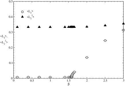
Figure 1: Vacuum expectation values of $L_{2}$ (gray circles) and $L_{2}^{2}$ (black triangles) at $8^{4}\times 8(L_{5}=4)$ lattice.

The $Z_{2}$-projected Polyakov loop (18) and its square have been computed on a $8^{4}\times 8$ lattice (namely, $L_{5}=4$) by using Monte-Carlo simulation with heatbath and overrelaxation algorithms (Fig. 1). Clearly, for $\beta<\beta_{c}\approx 1.6$, the vacuum expectation value (VEV) of the loop is vanishing and for $\beta>\beta_{c}$, it is increasing. $\beta_{c}$ is considered as a critical coupling. It is noted that not only the VEV of the loop but also that of square are very stable for $\beta<\beta_{c}$, whose coupling region implies the confining phase.

3 New symmetry and stick theorem

The argument of the previous section apparently leads to a conclusion that the $Z_{2}$-projected Polyakov loop is unsuitable for the order parameter of the center symmetry (17). The result of the Monte-Carlo simulation (Fig. 1), however, implies that there is a certain symmetry. We shall clarify the explicit form and the property of the symmetry in this section.

3.1 Stick transformation and new symmetry

At first, an expected transformation for link variables is independent of (15). The explicit form is

$$U^{\prime}_{{n_{M}},N}=\left\{\begin{array}[]{ll}\alpha(n_{\mu},I)U_{{n_{\mu}},\nu}(I)\alpha^{\dagger}(n_{\mu}+\hat{\nu},I)&{\rm for~{}links~{}on~{}}FP(I)~{},I=1,2~{},\\ \alpha(n_{\mu},1)U_{n_{M},5}&{\rm for~{}sticking~{}links~{}out~{}}FP(1)~{},\\ U_{{n_{M}},5}\alpha^{\dagger}(n_{\mu},2)&{\rm for~{}sticking~{}links~{}into~{}}FP(2)~{},\\ U_{{n_{M}},\nu}&{\rm for}~{}n_{5}=1,\cdots,L_{5}-1~{}{\rm with}~{}N=\nu~{},\\ U_{{n_{M}},5}&{\rm for}~{}n_{5}=1,\cdots,L_{5}-2~{}{\rm with}~{}N=5~{},\end{array}\right.$$ (19)

where $\alpha(n_{\mu},I)$ is an element of the $SU(2)$. Let us note that the above transformations are defined for the links on the orbifold $S^{1}/Z_{2}$, not on the $S^{1}$. The transformations for other links are determined by the $Z_{2}$ projection (2).

The first transformation of (19) must be careful in the consistency with (8),

$$g_{0}\alpha(n_{\mu},I)=\alpha(n_{\mu},I)g_{0}z(n_{\mu},I)~{}.$$ (20)

Here $z(n_{\mu},I)$ is an element of $SU(2)$ which commutes with any $U_{{n_{\mu}},\nu}(I)$ .

The action (7) is invariant under (19). This is because the plaquettes on the fixed points are invariant under the first transformation in (19) and the plaquette oriented for the fifth direction from the $FP(2)$

$$U_{P}=U_{\{n_{\mu},\,L_{5}-1\},\,5}U_{n_{\mu},\,\nu}(2)U^{\dagger}_{\{n_{\mu}+\hat{\nu},\,L_{5}-1\},\,5}U^{\dagger}_{\{n_{\mu},\,L_{5}-1\},\,\nu}$$ (21)

is also invariant under the first and the third transformations

$$U_{P}\rightarrow U_{P}^{\prime} = U_{\{n_{\mu},\,L_{5}-1\},\,5}\alpha^{\dagger}(n_{\mu},2)\alpha(n_{\mu},2)U_{n_{\mu},\,\nu}(2)\alpha^{\dagger}(n_{\mu}+\hat{\nu},\,2)$$ (22)

$$\qquad\times\alpha(n_{\mu}+\hat{\nu},\,2)U^{\dagger}_{\{n_{\mu}+\hat{\nu},\,L_{5}-1\},\,5}U^{\dagger}_{\{n_{\mu},\,L_{5}-1\},\,\nu}\,.$$

Hereafter we use the terminology, the FP gauge symmetry instead of the $U(1)$ gauge symmetry. It is important to note that the first transformation in (19) pulls the $U_{{n_{\mu}},\nu}(I)$ back to $U(1)$ of the FP gauge symmetry.

The explicit solutions for (20) are

$$\alpha(n_{\mu},I)=\left\{\begin{array}[]{ll}e^{i\theta(n_{\mu},I)\sigma_{3}}&{\rm~{}for~{}}z(I)=1{\rm~{}case}~{},\\ (i\sigma_{2})e^{i\theta(n_{\mu},I)\sigma_{3}}&{\rm~{}for~{}}z(I)=-1{\rm~{}case}~{},\\ {\rm no~{}solution}{}&{\rm~{}for~{}other~{}cases}~{}.\end{array}\right.$$ (23)

The first case in (23) just corresponds to the $U(1)$ gauge transformation (9). The second case is essentially a new global symmetry (up to the $U(1)$ gauge transformation). The consistency between (8) and (19) is confirmed as

$$g_{0}U^{\prime}_{n_{\mu},\nu}(I)g_{0}^{\dagger} = g_{0}\alpha(n_{\mu},I)U_{n_{\mu},\nu}(I)\alpha^{\dagger}(n_{\mu}+\hat{\nu},I)g_{0}^{\dagger}$$ (24)

$$= \alpha(n_{\mu},I)g_{0}z(n_{\mu},I)U_{n_{\mu},\nu}(I)z^{\dagger}(n_{\mu}+\hat{\nu},I)g_{0}^{\dagger}\alpha^{\dagger}(n_{\mu}+\hat{\nu},I)$$

$$= U^{\prime}_{n_{\mu},\nu}(I)~{},$$

where $[z(I),U_{n_{\mu},\nu}(I)]=[g_{0},U_{n_{\mu},\nu}(I)]=0$ has been used. This symmetry is global not local because the last equality in (24) holds only under the condition

$$z(n_{\mu},I)z^{\dagger}(n_{\mu}+\hat{\nu},I)=1~{}.$$ (25)

In order to obtain the nontrivial transformation for the $Z_{2}$-projected Polyakov loop $L_{2}(n_{\mu})$, we adopt $z(1)\neq z(2)$ as we will see below. Under our assignment of $z(1)=1$ and $z(2)=-1$, the transformation (19) (up to the $U(1)$ gauge transformation) becomes

$$U^{\prime}_{{n_{M}},N}=\left\{\begin{array}[]{ll}(i\sigma_{2})U_{n_{\mu},\nu}(2)(-i\sigma_{2})&{\rm for~{}links~{}on~{}}FP(2)~{},\\ U_{\{n_{\mu},0\},5}&{\rm for~{}sticking~{}links~{}out~{}}FP(1)~{},\\ U_{\{n_{\mu},L_{5}-1\},5}(-i\sigma_{2})&{\rm for~{}sticking~{}links~{}into~{}}FP(2)~{},\\ U_{{n_{M}},\nu}&{\rm for}~{}n_{5}=0,\cdots,L_{5}-1~{}{\rm with}~{}N=\nu~{},\\ U_{{n_{M}},5}&{\rm for}~{}n_{5}=1,\cdots,L_{5}-2~{}{\rm with}~{}N=5~{}.\end{array}\right.$$ (26)

Here link variables $U_{n_{\mu},\nu}(1)$ are transformed as the fourth case. This global transformation (26) is called as stick one, where we have defined a discrete transformation á la stick . Another assignment $z(1)=-1,z(2)=1$ is equivalent to (26) after the change of variable generating the exchange, $z(1)\leftrightarrow z(2)$.

The action (7) has four symmetries (9), (15), (17) and the new global symmetry (26) that we call the stick symmetry. With respected to the path-integral measure $dU_{{n_{\mu}},\nu}(2)$ for the stick transformation, we can understand the invariance from a fact that (26) induces an isomorphic map from a compact $U(1)$ into another compact $U(1)$ for link variables on $FP(2)$.

The $Z_{2}$-projected Polyakov loop is transformed nontrivially under (26) as

$$L^{\prime}_{2}(n_{\mu}) = {\rm Tr~{}}U_{\{n_{\mu},0\},5}\cdots U_{\{n_{\mu},L_{5}-1\},5}(-i\sigma_{2})g_{0}(i\sigma_{2})U^{\dagger}_{\{n_{\mu},L_{5}-1\},5}\cdots U^{\dagger}_{\{n_{\mu},0\},5}g_{0}^{\dagger}$$ (27)

$$= -L_{2}(n_{\mu}).$$

This means that the loop can be an order parameter for the stick symmetry. At first glance, the stick symmetry seems to be a subgroup of the bulk gauge symmetry, but it is never a gauge symmetry and is actually an independent global symmetry, as shown by (26) and (27). Here let us summarize the symmetry properties of the Polyakov loop in $S^{1},S^{1}/Z_{2}$ models under the center and stick transformations in Table I.

models	Polyakov loop	center symmetry	new (stick) symmetry
$S^{1}$	Tr $UUUU\cdots$	variant	not defined
$S^{1}/Z_{2}$	Tr $UU\cdots g_{0}U^{\dagger}U^{\dagger}\cdots g_{0}^{\dagger}$	invariant	variant

Table 1: Comparison between $S^{1}$ model and $S^{1}/Z_{2}$ model

3.2 Stick theorem and sticking operators

Correlation functions between two $Z_{2}$-projected Polyakov loops are important quantities since they may be related to Higgs fields and their masses. The new symmetry (26) controls not only the VEV of a single $Z_{2}$-projected Polyakov loop, but also the VEVs of the correlation function of the loops. The fundamental property of the VEVs of sticking operators into the $FP(2)$ (Fig. 2) is stated as a stick theorem:

A VEV of any product operators made from link variables sticking into the $FP(2)$ odd number of times vanishes unless the stick symmetry (26) is broken.

In order to prove this theorem, let us consider any operator $F(U)$ consisted of the link variables sticking into the $FP(2)$ odd number of times $N_{o}$

$$F(U)\equiv ({\rm Tr~{}}M_{1}U_{\{n_{\mu},L_{5}-1\},5}g_{0}U^{\dagger}_{\{n_{\mu},L_{5}-1\},5}M_{1}^{\dagger}g_{0}^{\dagger})\cdots$$ (28)

$$({\rm Tr~{}}M_{2}U_{\{n^{\prime}_{\mu},L_{5}-1\},5}g_{0}U^{\dagger}_{\{n^{\prime}_{\mu},L_{5}-1\},5}M_{2}^{\dagger}g_{0}^{\dagger})~{},$$

where $M_{1}$ and $M_{2}$ mean various product operators made from link variables detached from the $FP(2)$. We find by executing the change of variables with (26) that

$$<F(U)> = <F(U^{\prime})>$$ (29)

$$= \int\prod\limits_{n_{M},N}dU^{\prime}_{n_{M},N}e^{-S_{S^{1}/Z_{2}}(U^{\prime})}F(U^{\prime})\left/\int\prod\limits_{n_{M},N}dU^{\prime}_{n_{M},N}e^{-S_{S^{1}/Z_{2}}(U^{\prime})}\right.$$

$$= (-1)^{N_{o}}\int\prod\limits_{n_{M},N}dU_{n_{M},N}e^{-S_{S^{1}/Z_{2}}(U)}F(U)\left/\int\prod\limits_{n_{M},N}dU_{n_{M},N}e^{-S_{S^{1}/Z_{2}}(U)}\right.$$

$$= -<F(U)>~{},$$

where $S_{S^{1}/Z_{2}}(U)$ is an invariant plaquette action under (26). An equation (29) means that the VEV of the operator (28) vanishes if the stick symmetry (26) is unbroken.

q.e.d.

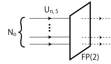
Figure 2: The $Z_{2}$-projected Polyakov loops sticking odd number of times into the fixed point $FP(2)$. The dashed arrows are related with $U_{n,5}$ by the $Z_{2}$ projection (2).

The simplest example of the sticking operator into the $FP(2)$ is the $Z_{2}$-projected Polyakov loop, which corresponds to the case with $N_{o}=1$ in Fig. $2$.

Furthermore, the sticking operators have some important properties for constructing the effective theory. The operators are stable against corrections in the strong coupling regime. The VEV of any product operator $F$ made from the link variables sticking into the $FP(2)$ locally odd number of times $N_{o}$ vanishes in the strong coupling limit owing to ${\rm~{}Tr~{}}g_{0}=0$ and $g_{0}^{2}=-1$. Here the locally  odd number of times means odd number of times sticking into a four-dimensional point on the $FP(2)$. But it admits the link variables to stick into the whole $FP(2)$ even number of times (Fig. 3). The typical example of such the operator is the correlation function of the $Z_{2}$-projected Polyakov loop. In the strong coupling limit, it is needless to consider any corrections for the plaquette.

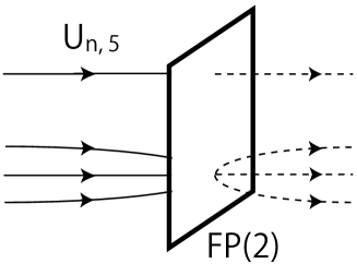
Figure 3: The $Z_{2}$-projected Polyakov loops sticking locally odd number of times into the fixed point $FP(2)$. The dashed arrows are related with $U_{n,5}$ by the $Z_{2}$ projection (2).

We also observe from Fig. 1 that $<L_{2}^{2}>$, which sticks locally even number of times into the $FP(2)$, seem to be very stable for $\beta<\beta_{c}$ . Before closing this section, it may be meaningful to state that the VEVs of the sticking operators into the $FP(2)$ always suppress any strong coupling corrections in the confining phase. This implies that the sticking operators are good candidates to describe the effective theory in the phase. These results are useful for constructing the effective theory, which will be discussed in the next section.

4 Effective theory and Elitzur’s theorem

Based on the new global symmetry (26), let us construct an effective theory from our lattice model in this section. Before proceeding with it, it may be instructive to mention the naive continuum (perturbative) limit of (2).

4.1 Naive continuum limit and an effective theory

If we write $U_{n_{M},N}={\rm exp}(iaA_{N}(n_{M}))$ in (2.1) and (5), then we find that boundary conditions for the gauge potential $A_{N}$,

$$A_{\nu}(n_{\mu},n_{5})=g_{0}A_{\nu}(n_{\mu},-n_{5})g_{0}^{\dagger}~{},\qquad A_{5}(n_{\mu},n_{5})=-g_{0}A_{5}(n_{\mu},-n_{5})g_{0}^{\dagger}~{}.$$ (30)

For $g_{0}=i\sigma_{3}$, the gauge symmetry is broken down to $U(1)$ by the orbifolding [10]. The zero modes in $A_{5}$, which are actually given by $A_{5}^{1}$ and $A_{5}^{2}$ from (30), play the role of the Higgs field in the gauge-Higgs unification. The Wilson line phase is an important quantity in the gauge-Higgs unification and can be written by the zero mode of the gauge potential $A_{5}$ (á la Higgs field). It is explicitly obtained by

$$W_{c}={\cal P}\mbox{exp}\left(ig_{5}\oint_{S^{1}/Z_{2}}dy\langle A_{5}\rangle\right)={\cal P}\mbox{exp}\left(ig_{5}\oint_{S^{1}/Z_{2}}dy\biggr{(}\langle A_{5}^{1}\rangle{\sigma_{1}\over 2}+\langle A_{5}^{2}\rangle{\sigma_{2}\over 2}\biggl{)}\right)~{},$$ (31)

where $g_{5}$ is the five-dimensional gauge coupling and ${\cal P}$ stands for the path-ordered product. We stress that the phase $W_{c}$ does not correspond to the loop (18), but to an operator $X(n_{\mu})$ defined below. As the result, the effective theory in the naive continuum limit can be expressed by $<A_{5}^{1}>,~{}<A_{5}^{2}>$ and $A_{\mu}^{3}$.

4.2 Elitzur’s theorem and its generalization

Since the notion of the gauge invariance is crucial on lattice, the physical picture based on the zero modes or the VEVs of gauge fields alone is useless because they are gauge variant quantities. The crucial point on lattice gauge theories is the existence of a theorem by Elitzur[14] on the VEV of a single link variable on lattice. The theorem precisely states that the VEV of the variable vanishes whenever the local symmetry is kept on lattice. For a composite operator made from link variables such as $U_{\{n_{\mu},L_{5}-1\},5}g_{0}U^{\dagger}_{\{n_{\mu},L_{5}-1\},5}g_{0}^{\dagger}$, a similar theorem holds except for the singlet component after the decomposition of the operator into irreducible representations, i.e., the VEV of the nontrivial components vanishes whenever the local symmetry is kept on lattice.

In our case, we need to generalize the Elitzur’s theorem to a five-dimensional lattice gauge theory with the FP gauge symmetries in the four-dimensional lattice spaces. A generalized statement on the Elitzur’s theorem follows as:

When we consider the lattice gauge transformation by the subgroup of an original gauge group, the VEVs of nontrivially gauge transformed operators are vanishing.

The proof of this generalization is essentially the same as Elitzur’s original one except for the consideration of the lattice gauge transformation corresponding to the subgroup.

From this generalization, we can understand that any FP gauge symmetry is always unbroken in the lattice gauge theory with the $Z_{2}$-orbifolding, because our FP gauge symmetry can be regarded as a subgroup of a bulk gauge transformation. The global stick symmetry is independent of the bulk gauge transformation and possible to be broken spontaneously.

4.3 Lattice effective theory

The effective theory must be constructed by gauge invariant operators such as a trace of the plaquette $U_{P}$ and a $Z_{2}$-projected Polyakov loop and by low-energy modes. Not only in a confining phase but also in a deconfining phase, these ’effective’ operators must be gauge invariant and/or must be the constituent parts of low-energy effective action with the gauge invariance on lattice. On the other hand, the zero modes of the component gauge fields for the fifth direction are important on the continuum theory. However, the zero mode is not gauge invariant, so that it cannot be consisted of a part of the low-energy effective action with the gauge invariance on lattice. Instead of the zero mode, we define an operator

$$X(n_{\mu})\equiv U_{\{n_{\mu},0\},5}U_{\{n_{\mu},1\},5}\cdots U_{\{n_{\mu},L_{5}-2\},5}U_{\{n_{\mu},L_{5}-1\},5}~{}.$$ (32)

It is noted that the $X(n_{\mu})$ is a bi-fundamental field for the FP gauge symmetry

$$X^{\prime}(n_{\mu})=e^{i\theta(n_{\mu},1)\sigma_{3}}X(n_{\mu})e^{-i\theta(n_{\mu},2)\sigma_{3}}~{},$$ (33)

and is transformed as

$$X^{\prime}(n_{\mu})=X(n_{\mu})(-i\sigma_{2})~{},$$ (34)

under the stick transformation. From (32), we can express the $Z_{2}$-projected Polyakov loop (18) as

$$L_{2}(n_{\mu})={\rm Tr~{}}X(n_{\mu})g_{0}X^{\dagger}(n_{\mu})g_{0}^{\dagger}~{},$$ (35)

which is clearly the FP gauge invariant and odd for the stick symmetry. From the discussion of the previous section including the stick theorem, the loop $L_{2}(n_{\mu})$ and the operator $X(n_{\mu})$ are very stable in the confining phase. And the effective potential for the loop should be an even function for the stick symmetry. For the pure $FP(I)$ gauge sector, the simplest FP gauge and stick symmetry invariant operators are traces of plaquette

$${\rm Tr~{}}U_{P}(I)\equiv{\rm Tr~{}}U_{n_{\mu},\nu}(I)U_{n_{\mu}+\hat{\nu},\rho}(I)U_{n_{\mu}+\hat{\rho},\nu}^{\dagger}(I)U_{n_{\mu},\rho}^{\dagger}(I)~{}{\rm~{}for~{}}I=1,2~{},$$ (36)

where the stick symmetry implies that

$$U^{\prime}_{n_{\mu},\nu}(1) = U_{n_{\mu},\nu}(1)~{},$$

$$U^{\prime}_{n_{\mu},\nu}(2) = (i\sigma_{2})U_{n_{\mu},\nu}(2)(-i\sigma_{2})=U^{*}_{n_{\mu},\nu}(2)~{}.$$ (37)

It is noted that the ${\rm Tr~{}}U_{P}(2)$ on the $FP(2)$ is real because the link variable $U_{n_{\mu},\nu}(2)$ belongs to the subgroup $U(1)$ of the $SU(2)$.

The first stage to construct the effective theory is to find massless or light modes. The massless modes are massless gauge fields associated with the FP gauge symmetry. The link variables which are variant under the $SU(2)$ bulk gauge symmetry (15) are path-integrated out. We assume that the variable $X(n_{\mu})$ defined by $(26)$, which is invariant under (15), is a fundamental operator in the effective theory. The second stage is to look for the form of the couplings among the modes. From the action (7), the link variable $U_{n_{\mu},\nu}(I)$ is coupled with staple products of the link variables which transform as the bi-fundamental representation of the FP gauge symmetry. Assuming that the staple products can be replaced by $X^{\dagger}(n_{\mu}+\hat{\nu})U^{\dagger}_{n_{\mu},\nu}(1)X(n_{\mu})$, the effective theory can be written as

$$S_{{\rm eff}} = \sum_{I=1,2}\beta_{I}{\rm Tr~{}}U_{n_{\mu},\nu}(I)U_{n_{\mu}+\hat{\nu},\rho}(I)U_{n_{\mu}+\hat{\rho},\nu}^{\dagger}(I)U_{n_{\mu},\rho}^{\dagger}(I)$$ (38)

$$+C\sum_{n_{\mu},\nu}{\rm Tr~{}}X^{\dagger}(n_{\mu}+\hat{\nu})U^{\dagger}_{n_{\mu},\nu}(1)X(n_{\mu})U_{n_{\mu},\nu}(2)+c.c$$

$$+\sum_{n_{\mu}\in FP{\rm s}}V\left({\rm Tr~{}}X(n_{\mu})(i\sigma_{3})X(n_{\mu})^{\dagger}(-i\sigma_{3})\right)~{},$$

where $c.c$ means the complex conjugation and $\beta_{I}$ and $C$ are coupling constants. The potential term $V(x)$ is an even function for the $Z_{2}$-projected Polyakov loop $X(n_{\mu})$ from the stick theorem.

The effective action (38) is invariant under the FP gauge and stick symmetries. The effective action suggests that the variable $X(n_{\mu})$ can be a candidate for the Higgs, which can play a role of a matter field in the fundamental representation of the FP gauge symmetry. Since $X(n_{\mu})$ belongs to the fundamental representation, the confinement phase is expected to be connected with a Higgs phase continuously from the Fradkin-Shenker’s discussion[15]. Contrary to the usual continuum theory, the effective theory has two sets of four-dimensional gauge fields. The gauge fields on the $FP(1)$ and $FP(2)$ interact with each other by mediating $X(n_{\mu})$. After solving the mixing, we may find a set of the four-dimensional gauge fields and of four-dimensional massive vector fields in the effective theory.

5 Summary and Discussions

In this paper, we have found a new symmetry (stick symmetry) on lattice gauge theory with $Z_{2}$-orbifolding. The symmetry and the associated theorem (stick theorem) control the behavior of an order parameter ($Z_{2}$-projected Polyakov loop) and restrict the form of the effective action. It is found that the operator $X(n_{\mu})$ behaves like the Higgs field in the effective action. The definition of a Higgs field on lattice is an important problem. The field should be the fundamental representation of the FP gauge symmetry. Although one of some candidates is $X(n_{\mu})$, better candidates should be determined by requirements: the simpler form and the smoothness for the continuum limit in calculating physical quantities such as Higgs mass.

When we consider an $SU(2)$ as the bulk gauge group, the stick symmetry belongs to a center in the $SU(2)$. One may wonder whether the stick symmetry is always the same as the center of a bulk gauge group or not. The answer is clearly no. When $SU(3)$ is considered as the bulk gauge symmetry, we need to adopt $g_{0}={\rm diag}(1,-1,-1)$ by $Z_{2}$-orbifolding, by which the bulk gauge symmetry is broken down to $SU(2)\times U(1)$ at the fixed points. In this case, we must generalize the new symmetry construction. We set a bulk gauge symmetry $G$. By $g_{0}\in G$, $G$ breaks down to a subgroup $H$ on the $FP(I)$

$$H\equiv\{g\in G|~{}g_{0}gg_{0}^{\dagger}=g\}~{}.$$ (39)

The normalizer $N_{G}(H)$ is defined as

$$N_{G}(H)\equiv\{g\in G|~{}ghg^{\dagger}=h^{\prime}\in H~{}{\rm for}~{}^{\forall}h\in H\}~{},$$ (40)

and $H$ is a normal subgroup of $N_{G}(H)$. It is clear that the stick transformation (26) is an element of $N_{G}(H)$ not $H$. More precisely, new symmetry up to the FP gauge symmetry is an element of the residual group $N_{G}(H)/H$. This residual group is discrete because $N_{G}(H)$ is isomorphic to $H$ as Lie groups. The $SU(3)$ case indicates that the residual group $N_{G}(H)/H$ is trivial not the center $Z_{3}$ of $SU(3)$. The change of the symmetry by $SU(3)$ has a serious influence on the role of the $Z_{2}$-projected Polyakov loop as an order parameter. With the $SU(N)$ bulk gauge symmetry, we find VEV of the loop,

$$<L_{2}>\rightarrow\frac{|{\rm~{}Tr~{}g_{0}}|^{2}}{N}~{},$$ (41)

in the strong coupling limit. Since ${\rm Tr~{}g_{0}}$ is $-1$ in the $SU(3)$ case, $<L_{2}>$ is non-vanishing in the limit. From this fact, it is difficult to treat $L_{2}(n_{\mu})$ as the order parameter for the stick symmetry generally. For general bulk gauge groups, the construction of its new symmetry is an open question.

In the relation of our lattice model to the continuum theory, we have to make a few comments. In this article, we have considered the lattice model as a cutoff theory following to Irges and Knechtli[11, 12, 13]. Although it is generally difficult to take the continuum limit of lattice models, the realization of the limit is expected by the 2nd order phase transition. The further analysis of the phase structure of the $S^{1}/Z_{2}$-orbifolded gauge theory may open its possibility.

References

- [1] N. S. Manton, \NPB158,1979,141.
- [2] D. B. Fairlie, \PLB82,1979,97.
- [3] Y. Hosotani, \PLB126,1983,309; \ANN190,1989,233.
- [4] N. V. Krasnikov, \PLB273,1991,731, H. Hatanaka, T. Inami and C. S. Lim, Mod. Phys. Lett. A13 (1998) 2601, G. R. Dvali, S. Randjbar-Daemi and R. Tabbash, \PRD65,2002,064021, N. Arkani-Hamed, A. G. Cohen and H. Georgi, \PLB513,2001,232, I. Antiniadis, K. Benakli and M. Quiros, New J. Phys. 3,(2001),20.
- [5] K. Takenaga, \PRD64,2001,066001; \PRD66,2002,085009, N. Haba and Y. Shimizu, \PRD67,2003,095001, C. Csaki, C. Grojean, H. Murayama, \PRD67,2003,085012, I. Gogoladze, Y. Mimura, S. Nandi and K. Tobe, \PLB575,2003,66, C. Csaki, C. Grojean, H. Murayama, L. Pilo and J. Terning, \PRD69,2004,055006, K. Choi, N. Haba, K. S. Jeong, K. Okumura, Y. Shimizu and M. Yamaguchi, \JHEP0402,2004,037, Y. Hosotani, S. Noda and K. Takenaga, \PRD69,2004,125014; \PLB607,2005,276, N. Haba, K. Takenaga and T. Yamashita, \PRD71,2005,025006, G. Panico, M. Serone and A. Wulzer, \NPB739,2006,186, G. Panico and M. Serone, \JHEP0505,2005,024, N. Maru and K. Takenaga, \PRD72,2006,046003; \PRD74,2006,015017.
- [6] Y. Hosotani, arXiv: 0809.2181[hep-ph], M. Carena, A. D. Medina, N. R. Shah and C. E. M. Wagner, arXiv:0901.0609[hep-ph], Y. Mimura, arXiv:0903.1875[hep-ph], F. Brümmer, S. Fichet, A. Hebecker and S. Kraml, arXiv:0906.2957[hep-ph].
- [7] A. T. Davies and A. McLachlan, \PLB200,1988,305; \NPB317,1989,237, J. E. Hetrick and C. L. Ho, \PRD40,1989,4085, A. Higuchi and L. Parker, \PRD37,1988,2853, C. L. Ho and Y. Hosotani, \NPB345,1990,445, A. McLachlan, \NPB338,1990,188, K. Takenaga, \PLB425,1998,114; \PRD58,1998,026004.
- [8] A. Masiero, C. A. Scrucca, M. Serone and L. Silvestrini, \PRL87,2001,251601.
- [9] Y. Hosotani, N. Maru, K. Takenaga and T. Yamashita, \PTP118,2007,1053.
- [10] M. Kubo, C. S. Lim and H. Yamashita, Mod. Phys. Lett. A17 (2002) 2249, L. J. Hall, Y. Nomura and D. R. Smith, \NPB639,2002,307, G. Burdman and Y. Nomura, \NPB656,2003,3.
- [11] N. Irges and F. Knechtli, \NPB719,2005,121.
- [12] N. Irges and F. Knechtli, hep-lat/0604006.
- [13] N. Irges and F. Knechtli, \NPB775,2007,283.
- [14] S. Elitzur, \PRD12,1975,3978.
- [15] E. Fradkin and S. H. Shenker, \PRD19,1979,3682.