Long-term Photometric Behavior of the Eclipsing Binary GW Cephei

Abstract

New CCD photometry during 4 successive years from 2005 is presented for the eclipsing binary GW Cep, together with reasonable explanations for the light and period variations. All historical light curves, obtained over a 30-year interval, display striking light changes, and are best modeled by the simultaneous existence of a cool spot and a hot spot on the more massive cool component star. The facts that the system is magnetically active and that the hot spot has consistently existed on the inner hemisphere of the star indicate that the two spots are formed by (1) magnetic dynamo-related activity on the cool star and (2) mass transfer from the primary to the secondary component. Based on 38 light-curve timings from the Wilson-Devinney code and all other minimum epochs, a period study of GW Cep reveals that the orbital period has experienced a sinusoidal variation with a period and semi-amplitude of 32.6 yrs and 0.009 d, respectively. In principle, these may be produced either by a light-travel-time effect due to a third body or by an active magnetic cycle of at least one component star. Because we failed to find any connection between luminosity variability and the period change, that change most likely arises from the existence of an unseen third companion star with a minimum mass of 0.22 $M_{\odot}$ gravitationally bound to the eclipsing pair.

1 INTRODUCTION

After GW Cep (CSV 5941, BV 7, 2MASS J01455862+8004553) was discovered to be a variable star by Strohmeier (Geyer et al. 1955), its light curves were made photoelectrically by Meinunger & Wenzel (1965), Hoffmann (1982), Landolt (1992), and Pribulla et al. (2001). They recognized it as a W-subtype (defined empirically by Binnendijk (1970)) eclipsing binary with complete eclipses. Kaluzny (1984) analyzed Hoffmann’s $BV$ light curves by using Rucinski’s (1976) code and concluded that the binary is an over-contact system with the characteristic parameters of $q$=2.703 and $i$=83${}^{\circ}.9$ and a fill-out factor $f$=11.3 %. Pribulla et al. analyzed their own $BV$ light curves using the Wilson & Devinney (1971, hereafter W-D) code. Except for a value of $f$=23.5 %, their results are very similar to those of the earlier study. The orbital period of GW Cep has been examined by Pribulla et al. and Qian (2003), who reported that the period is decreasing. More recently, Chochol et al. (2006) suggested that the variation of the orbital period could be produced by two possible forms: a single light-travel time (LTT) ephemeris with and without a quadratic term.

Although GW Cep has been studied photometrically these several times, intrinsic light variations due to starspots have not yet been considered. Additionally, the period variation still has not been described as conclusively as can be desired. In this paper, we present and discuss the long-term photometric behavior of the binary system from detailed studies of all available data.

2 NEW EXTENDED CCD PHOTOMETRY

We carried out CCD photometric observations of GW Cep on 20 nights from 2005 October through 2008 November in order to look for possible long-term light variability. The observations were taken with a SITe 2K CCD camera and a $BVR$ filter set attached to the 61-cm reflector at Sobaeksan Optical Astronomy Observatory (SOAO) in Korea. The exposure times were about 40$-$85 s for $B$, 20$-$40 s for $V$, and 10$-$20 s for $R$ with a 2$\times$2 binning mode. The individual choices depended on the seeing and transparency of the night sky. The instrument and reduction method have been described by Lee et al. (2007a). A summary of the observations is given in Table 1, where we present seasonal observing intervals, filters, numbers of observed points, and designations for all datasets.

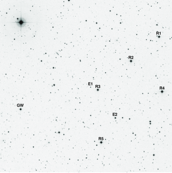
Figure 1: An observed CCD image (20$\arcmin$.5$\times$20′.5) of GW Cep and many nearby stars. E1 and E2 are eclipsing binary systems named CzeV106 Cep (GSC 4502-1040) and CzeV079 Cep (GSC 4502-0138), respectively. Monitoring numerous frames led us to choose R2 as a comparison star. North is up and east is to the left.

An image of the observing field appears in Figure 1, with the eclipsing variable designated as GW and candidate comparison stars marked as Rn (n being a sequence number). Since an individual frame was large enough to image a few tens of nearby stars simultaneously, we monitored many of them on each frame. To find a comparison star that would be optimal for long-term observing, we first took an average of 5 potentially useful field stars calling that average $<$R$>$ and examined each field star against $<$R$>$ as a reference. The R1 and R3 stars showed excessive noise and were therefore excluded as possible comparison candidates. Candidates R4 and R5 did not appear to be variable but their noise levels against $<$R$>$ were larger than was the case for R2. Ultimately, R2 (2MASS J01405717+8011069, GSC 4502-0542, TYC 4502-542-1; $V\rm_{T}$=$+$10.82, $(B-V)\rm_{T}$=$+$0.94) was chosen as a suitable comparison star (C). The 1$\sigma$-value of the dispersion of the (C$-<$R$>$) differences is about $\pm$0.006 mag.

A total of 4,227 individual observations was obtained among the three bandpasses (1414 in $B$, 1416 in $V$, and 1397 in $R$) and a sample of them is listed in Table 2. The light curves are plotted in Figure 2 as differential magnitudes versus orbital phase.

3 THE LIGHT CURVES AND SPOTS MODELS

Figure 2 displays a quite active light curve for GW Cep. Most observations show the conventional O’Connell effect with Max I (at phase 0.25) brighter than Max II. Our light curves were solved in a manner similar to that for TU Boo (Lee et al. 2007b) and AR Boo (Lee et al. 2009a) by using contact mode 3 of the W-D code. In order to obtain an unique set of photometric solutions, our light-curve synthesis was carried out in two stages. In the first stage, all SOAO observations were analyzed simultaneously without a spot. In the second stage, the existence of short-time brightness disturbances caused us to model separately each dataset (designated in the fifth column of Table 1) by assuming the unspotted solutions and by adjusting only spot and luminosity parameters.

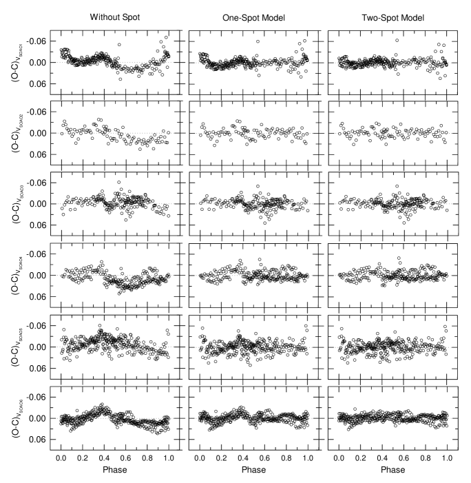
Figure 3: The left, middle, and right panels show the light residuals from the solutions without a spot, with a one-spot model, and with a two-spot model listed in Tables 3 and 4, respectively. The data refer to the $V$ bandpass.

The surface temperature of the more massive star was held fixed at 5800 K, appropriate for its spectral type G3 (Meinunger & Wenzel 1965). Linear bolometric ($X$) and monochromatic ($x$) limb-darkening coefficients were initialized from the values of van Hamme (1993) and were used together with the model atmosphere option. From a detailed $q$-search procedure over the range of 0.3 $\leq q\leq$ 4.0, we found that the sum of the weighted squared residuals, $\Sigma W(O-C)^{2}$, reached a minimum around $q$=2.60. That indicates that GW Cep is indeed a W-subtype contact binary as previous workers had found. The initial value of $q$ was then treated as an adjustable parameter to derive the unspotted solution listed in Table 3, wherein the primary and secondary stars refer to those being eclipsed at Min I and Min II, respectively. Therefore, the latter star is the cooler, larger, and more massive component. The $V$ residuals from the analysis are plotted in the left panels of Figure 3. Similar patterns exist for the other bandpasses.

As can be seen from these panels, the model light curves do not fit the observed ones at all well. The discrepancies resemble those of solar-type contact binaries recently studied such as TU Boo, AR Boo, and BX Peg (Lee et al. 2009b), for which non-modelled light could be explained by spot variability on the stellar photospheres. This condition could result from magnetic dynamo-related activity and/or variable mass transfer between the components. Because our long-term data show conspicuous seasonal light variations despite a constant value of $f$, it is more reasonable to regard the main cause of the second-order activity to be a magnetized cool spot on either component star of GW Cep rather than sporadically-variable mass transfer. Adopting the light curves of SOAO6 as reference ones, we tested a single cool spot on each component. A cool spot on the larger secondary star gives a slightly smaller value of $\Sigma W(O-C)^{2}$ than if the spot were on the primary. This is consistent with Mullan’s (1975) suggestion that the more massive components of contact binaries would preferentially manifest starspots. Therefore, we solved each SOAO dataset separately using the cool-spot model. The results are given as the one-spot model of Table 4 and the light residuals from this model are plotted in the central panels of Figure 3. It shows that a single cool spot on the secondary component does improve the light-curve fitting greatly but brightness disturbances are still conspicuous around phase 0.38. This detail can be interpreted by introducing a hot spot on the surface of the secondary as was verified by testing the SOAO6 data for this possibility. Lastly, all SOAO light curves were re-analyzed by using a two-spot model with both a cool spot and a hot spot on the secondary star. The final result is listed in the two-spot-model entries of Table 4 and the residuals from this model are plotted in the right panels of Figure 3. Although not perfectly flat with respect to phase, this distribution of residuals is a great improvement over the previous one.

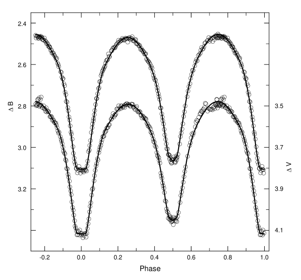
Figure 4: The $BV$ light curves of Hoffmann. The continuous curves represent the solutions obtained with the model parameters listed in columns (2)-(3) of Table 5.

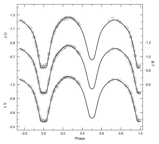
Figure 5: The $UBV$ light curves of Landolt. The continuous curves represent the solutions obtained with the model parameters listed in columns (4)-(5) of Table 5.

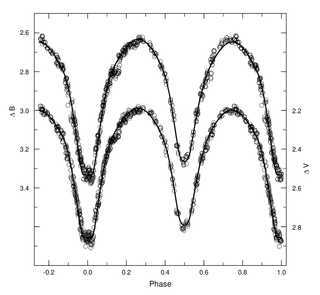
Figure 6: The $BV$ light curves of Pribulla et al. The continuous curves represent the solutions obtained with the model parameters listed in columns (6)-(7) of Table 5.

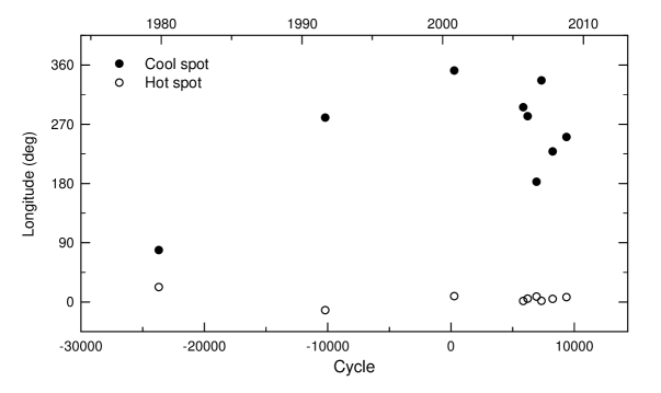
Figure 7: Changes of the cool- and hot-spot longitudes versus time from our two-spot model.

To study the long-term spot behavior of GW Cep, we analyzed the historical light curves by using our photometric parameters listed in Table 3 and adopting a two-spot model for the more massive secondary component. The data of Meinunger & Wenzel (1965) could not be included in our analysis because they remain unavailable. The model parameters for the datasets of Hoffmann (1982), Landolt (1992), and Pribulla et al. (2001) lead to the continuous curves in Figures 4–6 and appear in Table 5. Although Landolt’s observations have a large gap between phases 0.37 and 0.68, his light curves were actually modeled for spot descriptions. It can be seen that the stellar brightness ratios have not changed as a result of the spot modeling and it can also be seen that, in the 2000 data by Pribulla et al., the cool spot had almost disappeared. From the analyses, we conclude that the two-spot model satisfies all GW Cep curves quite well and gives a good representation of the binary system for both the photospheric and spot descriptions. As seen in Tables 4 and 5 and Figure 7, our results indicate that the long-term light variations are dominated by the changes of the cool spot with time, especially by a longitude drift of that spot. Because its position on the inner hemisphere of the secondary star has not changed appreciably over the 30-year interval, the hot spot can be produced by stable mass transfer from the less massive primary impacting on the more massive secondary component. Thus, the intrinsic light variations of GW Cep have been modeled by the simultaneous existence of the active cool spot on the secondary star and an enduring hot spot due to mass transfer between the components. In all the procedures that have been described, we did not look for a possible third light source as might be suggested by the orbital period study now to be described.

Identifying a satisfactory comparison star is critical to the credibility of the spot descriptions. Had we, for instance, chosen R1 as the comparison star, a light modulation of a bit less than 0.02-mag peak-to-peak would have been introduced into the sequence of light curves and this could well have been attributed to a third spot with a cycle length of about 3 years.

4 ORBITAL PERIOD STUDY

Times of minimum light may be shifted from conjunction instants by asymmetrical eclipse minima due to spot activity (cf. Lee et al. 2009a). Because 9 datasets of GW Cep were modeled for spot parameters, we calculated a minimum epoch for each eclipse in these datasets with the W-D code by means of adjusting only the ephemeris epoch ($T_{0}$). Thirty-eight such timings of minimum light are given in Table 6, together with those previously known or newly determined using the method of Kwee & van Woerden (1956, hereafter KvW) for comparison. Two of these (HJD 2,444,289.27664 and 2,451,884.61130) have been derived by us from the individual measurements. As in the case of AR Boo, there are systematic runs of differences between the KvW timings and the W-D ones. For SOAO6 and probably for SOAO2-5 as well, the differences are negative for Min I and positive for Min II except for two eclipses (HJD 2,454,026.99936 and 2,454,421.07651). These differences are caused by the cool spot and the hot spot presented to the observer before Min I and Min II, respectively. A total of 156 minimum timings over 45 years (50 visual, 6 photographic, 24 photoelectric, and 76 CCD), including the new W-D timings, were used to study the orbital period. For ephemeris computations, the following standard deviations were assigned to timing residuals based on the observational technique and the method of measuring the epochs: $\pm$0.0068 d for visual and photographic, $\pm$0.0012 d for photoelectric, $\pm$0.0008 d for CCD, and $\pm$0.0004 d for W-D minima. Relative weights were then scaled from the inverse squares of these values.

From a parabolic least-squares fit, Pribulla et al. (2001) suggested that their measured period decrease can be driven by mass transfer from the more to the less massive component but may also be inflected by an LTT effect caused by the presence of a third companion physically bound to the eclipsing pair. The reason for this conclusion is that the sum of the weighted squared residuals from a 3rd-order polynomial fit is 7 % lower than for a 2nd-order one. Chochol et al. (2006) reported that the orbital period changes of the binary system can be represented by either a single LTT ephemeris or by a combination of a downward parabola and an LTT (i.e., a quadratic plus LTT ephemeris). To find the best representation, We fitted all minimum epochs to several ephemeris forms including those already tried and found that the single LTT ephemeris gives a satisfactory representation without needing a quadratic term:

$$C=T_{0}+PE+\tau_{3},$$ (1)

where $\tau_{3}$ is the LTT due to a third body (Irwin 1952, 1959) and includes five parameters ($a\sin i_{3}$, $e$, $\omega$, $n$, $T$). The Levenberg-Marquart technique (Press et al. 1992) was applied to solve for the parameters of the ephemeris. The result is plotted in Figure 8 and orbital parameters are summarized in Table 7, together with the third-body masses ($M_{3}$) calculated for three different values of $i_{3}$. Absolute dimensions by Maceroni & van’t Veer (1996) have been used for these and subsequent calculations. The orbital eccentricity is not significant.

If the hypothetical third companion is a normal main-sequence star and its orbit is coplanar with the eclipsing pair ($i_{3}$ = 85${}^{\circ}.4$), the mass of the object is $M_{3}$ = 0.22 M_⊙ and its radius is calculated to be $R_{3}$ = 0.23 R_⊙ from the empirical mass-radius relation of Bayless & Orosz (2006). These correspond to a spectral type of about M6-7 and a bolometric luminosity of $L_{3}$ = 0.004 L_⊙. This small value compared to the larger intrinsic variability due to variable spots is the reason no “third light” was sought in our analyses.

Because there is no independent evidence to support the LTT hypothesis, one must consider the alternative: a period modulation due to a magnetic activity cycle, as initially proposed by Applegate (1992) and later modified by Lanza et al. (1998). According to this model, a change in the distribution of angular momentum of a magnetically active star causes a change in the star’s gravitational quadratic moment and hence forces a modulation of the orbital period. To obtain the model parameters for possible magnetic activity, we applied the period ($P_{3}$) and amplitude ($K$) to Applegate’s formulae. The results from these calculations are presented in Table 8 and correspond to typical values for contact binaries. Here, the quantity $\Delta m_{\rm rms}$ denotes a bolometric magnitude difference calculated from the equation (4) of Kim et al. (1997).

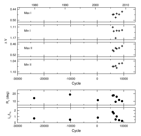
Figure 9: The four panels at the top display the $\Delta V$ variations for GW Cep at selected phases. The fifth and sixth panels represent the changes of the radius ($\rm R_{c}$) of the cool spot and of the luminosity ratio ($\rm L_{c}/L_{h}$) between the cool and hot spots, respectively, from our two-spot model.

According to the prediction of the Applegate model, the brightness variation of a binary should vary in a pattern and sense similar to the period change seen in the $O$–$C$ diagram. In order to study this possibility, we measured the light levels at four special phases for the GW Cep light curves. The $\Delta V$ variations for only the SOAO data are plotted in the first through fourth panels of Figure 9 because the other datasets used different comparison stars and could not be made comparable to the zero points of the SOAO light curves. The light level at Max II, plotted in the third panel, has brightened in tandem with the period increase over the interval of monitoring but the other light levels fail the test. To look for any further connection between spot variability and orbital period changes, we examined the changes with time of the radius ($\rm R_{c}$) of the cool spot and of the luminosity ratio ($\rm L_{c}/L_{h}$) between the cool and hot spots from our two-spot model. These have been assembled in the fifth and sixth panels of Figure 9, respectively. There clearly exists a variation in the size of the cool spot but the changes in its parameters do not conform to Applegate’s prediction. At present, we do not know what would be the appearance of a complete cycle for the cool spot because data are insufficient. It is also possible that magnetic activity is not constant, as already suggested by us for AR Boo, but the weight of present evidence favors a 3rd-body interpretation rather than a magnetic-cycle one for the period modulation.

This is the second in our series of contact binary studies in which we have used timings developed from the W-D code. As Figure 8 in this study and Figure 2 accompanying the paper on AR Boo show, this method is superior to all others: if the ordinate scale of an $O$–$C$ diagram is chosen so as to make obvious the noise in visual or photographic timings, the noise in photoelectric and conventional CCD timings will also be detectable but that from W-D determinations will not be obvious to even detailed inspection of the printed page. The weight of such timings will be the most powerful determinant in fitting the timing residuals. This understanding must become part of any program decision of whether simply to monitor minimum timings or to develop entire light curves whereby the bias due to photospheric spots may be removed from the timings. Only in this way will large and small secular and cyclical terms be evaluated to the highest accuracy and it be possible to decide if the cyclical terms are really periodic.

5 SUMMARY AND DISCUSSION

New multiband CCD light curves plus historical ones all display complete eclipses leading to system descriptions of high weight. The O’Connell effect and superposed long-term light variability are best explained by both a cool spot and a hot one on the more massive secondary star. The long-term variability has been ascribed to changes in the size of the cool spot. This spot may be produced by magnetic dynamo-related activity because the system is rotating rapidly and has a common convective envelope. The hot spot, on the other hand, is likely caused by impact from mass transfer between the components.

Over 45 years, the orbital period change of GW Cep has shown a periodic oscillation with a cycle length of 32.6 yr and a semi-amplitude of 0.009 d. In principle, this oscillation may be produced either by an LTT effect due to an unseen third star with a scaled mass of $M_{3}\sin i_{3}$=0.22 $M_{\odot}$ or by an active magnetic cycle in the more massive secondary star. We indicate that the latter interpretation is the less likely of the two possibilities.

With a relatively favorable light ratio and complete eclipses GW Cep clearly merits a radial velocity determination. Those eventual results will add weight to understanding the entire class of contact binaries but is there anything about the binary which appears singular at the present time? One item which attracts attention is the unfamiliar finding that the Keplerian period has been constant over 45 years. This may be examined in some detail from The Atlas of $O$–$C$ Diagrams of Eclipsing Binary Stars (Kreiner et al. 2001). From that source we extracted the period histories of all cool contact binaries which have periods shorter than that of GW Cep. These systems number 32 (1 A-type, 25 W-types and 6 not presently classified) and the shortest period is 0.221 d. In order to complete a sample for which GW Cep will have the median period, we next found the 32 contact binaries which show successively longer periods. These 32 systems are apportioned among 11 A-types, 17 W-types and 4 presently unclassified and the longest period is 0.365 d. Of this total sample of 65 pairs, 6 (AT Aqr, GW Cep, V906 Cyg, V743 Sgr, RZ UMi and BP Vel) appear at present to show constant periods. The remainder show secularly variable periods of either algebraic sign upon which bounded oscillations are superposed in some cases. Clearly, constant periods are an uncommon phenomenon in the sample and one may conjecture that they signify brief episodes of constant period behavior during themal oscillation evolutionary events. Of the 6 binaries, all but GW Cep have poor continuity in their period histories leaving that object as the best system at present to test such a possibility. Not only GW Cep, but the 5 other binaries merit continuing period monitoring.

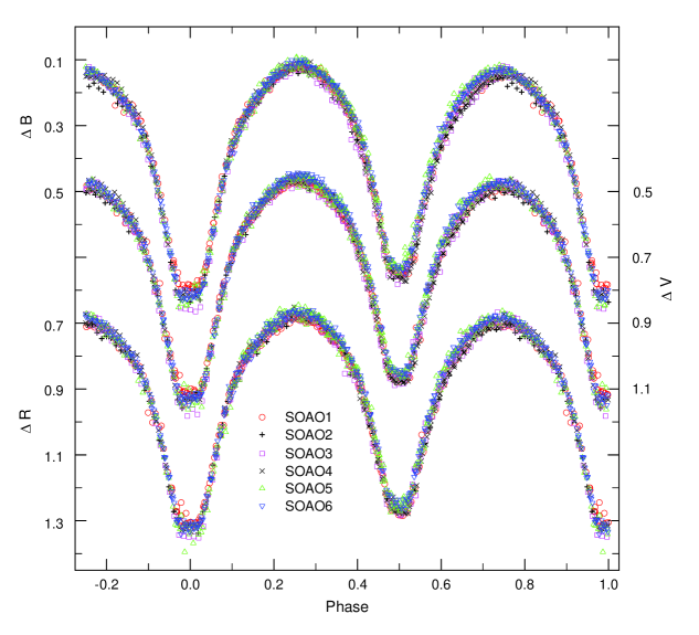
Figure 2: SOAO light curves of GW Cep in the $B$, $V$, and $R$ bandpasses defined by individual observations.

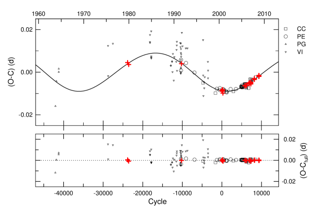
Figure 8: The $O$–$C$ diagram of GW Cep. In the upper panel, constructed with the linear terms in Table 7, the continuous curve represents the LTT orbit. The residuals from the complete ephemeris are plotted in the lower panel. Plus symbols refer to new minimum timings obtained with the W-D code.

Table 1: Summary of the SOAO observations of GW Cep.

UT Date	Observing Interval	Filter	$N_{\rm obs}$	Note
	(HJD+2,450,000)
2005 Oct. 19, 20, 22, 23	3663.04$-$3667.06	$BVR$	796	SOAO1
2006 Feb. 11	3777.95$-$3778.29	$BVR$	271	SOAO2
2006 Sep. 10, 13, Oct. 18	3989.00$-$4027.07	$BVR$	576	SOAO3
2007 Jan. 29, Feb. 2, 6, 7	4129.92$-$4139.08	$BVR$	664	SOAO4
2007 Nov. 16, 17, 18, 24	4420.92$-$4429.38	$BVR$	892	SOAO5
2008 Nov. 5, 9, 10, 18, 19	4775.94$-$4790.21	$BVR$	1028	SOAO6

Table 2: CCD photometric observations of GW Cep.

HJD	$\Delta B$	HJD	$\Delta V$	HJD	$\Delta R$
2,453,663.04074	0.724	2,453,663.03811	0.992	2,453,663.03915	1.207
2,453,663.04413	0.781	2,453,663.04197	1.068	2,453,663.04298	1.272
2,453,663.04755	0.784	2,453,663.04536	1.117	2,453,663.04637	1.315
2,453,663.05093	0.794	2,453,663.04876	1.110	2,453,663.04976	1.309
2,453,663.05433	0.787	2,453,663.05215	1.117	2,453,663.05316	1.305
2,453,663.05769	0.798	2,453,663.05556	1.118	2,453,663.05656	1.318
2,453,663.06095	0.785	2,453,663.05887	1.112	2,453,663.05985	1.297
2,453,663.06424	0.744	2,453,663.06214	1.085	2,453,663.06311	1.257
2,453,663.06749	0.674	2,453,663.06541	1.056	2,453,663.06637	1.221
2,453,663.07075	0.596	2,453,663.06866	0.979	2,453,663.06964	1.158

Note. — This table is available in its entirety in machine-readable and Virtual Observatory (VO) forms in the online journal. A portion is shown here for guidance regarding its form and content.

Table 3: GW Cep parameters obtained by fitting simultaneously all SOAO data.

Parameter	Primary	Secondary
$T_{0}$ (HJD)	2,453,322.22167$\pm$0.00007
$P$ (d)	0.31883212$\pm$0.00000002
$q$ (=ms/mp)	2.590$\pm$0.008
$i$ (deg)	85.4$\pm$0.2
$T$ (K)	6104$\pm$3	5800
$\Omega$	5.960$\pm$0.009	5.960
$f$ (%)	17.6
$A$	0.5	0.5
$g$	0.32	0.32
$X$	0.493	0.506
$x_{B}$	0.743$\pm$0.008	0.664$\pm$0.007
$x_{V}$	0.552$\pm$0.009	0.620$\pm$0.007
$x_{R}$	0.462$\pm$0.009	0.573$\pm$0.008
$L/(L_{1}+L_{2})_{B}$	0.357$\pm$0.001	0.643
$L/(L_{1}+L_{2})_{V}$	0.353$\pm$0.001	0.647
$L/(L_{1}+L_{2})_{R}$	0.347$\pm$0.001	0.653
$r$ (pole)	0.2881$\pm$0.0009	0.4435$\pm$0.0007
$r$ (side)	0.3015$\pm$0.0011	0.4756$\pm$0.0009
$r$ (back)	0.3404$\pm$0.0020	0.5052$\pm$0.0012
$r$ (volume)a	0.3119	0.4763
$\Sigma W(O-C)^{2}$	0.0137

Table 4: Spot and luminosity parameters for each SOAO dataset.

Parameter	SOAO1		SOAO2		SOAO3		SOAO4		SOAO5		SOAO6
Mean Year	2005.8		2006.1		2006.7		2007.1		2007.9		2008.9
Mean Epoch	5851		6206		6927		7324		8235		9358
One-Spot Model
Phase shifta	$-$0.0004(1)		$-$0.0006(3)		$-$0.0009(2)		$-$0.0017(2)		0.0006(2)		0.0014(1)
Colatitude2 (deg)	72.2(1.1)		72.7(5.6)		79.7(3.2)		79.7(6)		76.8(3.4)		74.8(6)
Longitude2 (deg)	292.5(1.1)		273.2(5)		181.8(1.3)		327.5(3.6)		227.3(2.2)		240.0(1.1)
Radius2 (deg)	16.8(3)		17.7(1.5)		9.5(5)		14.4(4)		13.0(5)		13.6(2)
$T$spot,2/$T$local,2	0.880(7)		0.881(9)		0.870(20)		0.870(6)		0.846(13)		0.845(6)
$L_{1}/(L_{1}+L_{2})_{B}$	0.3567(3)		0.3567(5)		0.3567(4)		0.3567(3)		0.3567(3)		0.3567(2)
$L_{1}/(L_{1}+L_{2})_{V}$	0.3530(3)		0.3530(5)		0.3529(4)		0.3529(3)		0.3529(3)		0.3530(2)
$L_{1}/(L_{1}+L_{2})_{R}$	0.3470(3)		0.3471(5)		0.3471(4)		0.3471(3)		0.3471(3)		0.3471(2)
$\Sigma W(O-C)^{2}$	0.0100		0.0103		0.0116		0.0096		0.0132		0.0085
Two-Spot Model
Phase shifta	$-$0.0008(1)		$-$0.0016(3)		$-$0.0013(2)		$-$0.0020(1)		$-$0.0002(2)		$-$0.0002(1)
Colatitude2 (deg)	75.6(8)	69.9(2.7)	75.6(0.9)	69.9(1.3)	80.0(1.1)	79.7(3.1)	77.9(9)	77.2(7)	77.2(4)	75.8(4.0)	76.2(3)	76.2(3.6)
Longitude2 (deg)	1.4(1.0)	295.8(2.0)	4.9(1.1)	282.3(3.0)	8.1(1.0)	182.7(4.1)	1.6(5)	336.6(6)	4.7(1.2)	228.7(2.4)	7.3(4)	250.6(3.2)
Radius2 (deg)	8.0(6)	17.5(5)	8.0(5)	17.8(6)	7.9(7)	9.4(5)	8.1(3)	16.0(2)	9.7(4)	11.7(1.0)	10.6(2)	10.2(3)
$T$spot,2/$T$local,2	1.145(14)	0.892(6)	1.195(25)	0.892(8)	1.110(15)	0.870(20)	1.235(15)	0.884(5)	1.173(9)	0.861(14)	1.170(5)	0.879(9)
$L_{1}/(L_{1}+L_{2})_{B}$	0.3567(3)		0.3567(4)		0.3567(3)		0.3567(3)		0.3567(3)		0.3567(2)
$L_{1}/(L_{1}+L_{2})_{V}$	0.3530(3)		0.3530(4)		0.3530(4)		0.3529(3)		0.3529(3)		0.3530(2)
$L_{1}/(L_{1}+L_{2})_{R}$	0.3471(3)		0.3471(4)		0.3471(4)		0.3471(3)		0.3471(3)		0.3471(2)
$\Sigma W(O-C)^{2}$	0.0098		0.0095		0.0114		0.0091		0.0126		0.0072

Table 5: Spot and luminosity parameters for historical light curves.

Parameter	Hoffmann (1982)			Landolt (1992)		Pribulla et al. (2001)
Mean Year	1980.0			1991.8		2000.9
Mean Epoch	$-$23695			$-$10208		261
$T_{0}$ (HJD)	2,444,200.48198$\pm$0.00006			2,448,544.87119$\pm$0.00008		2,451,799.48430$\pm$0.00006
$P$ (day)	0.3188288$\pm$0.0000005			0.318851025a		0.3188282$\pm$0.0000003
Colatitude2 (deg)	67.0$\pm$4.7	71.8$\pm$1.1		76.2$\pm$1.6	74.8$\pm$3.7	78.9$\pm$0.5	80.1$\pm$4.4
Longitude2 (deg)	22.5$\pm$2.2	78.8$\pm$1.8		347.5$\pm$1.1	280.1$\pm$1.3	8.8$\pm$0.4	351.6$\pm$5.4
Radius2 (deg)	10.7$\pm$0.8	14.1$\pm$0.3		12.8$\pm$0.5	18.8$\pm$0.6	7.1$\pm$0.3	11.5$\pm$2.3
$T$spot,2/$T$local,2	1.063$\pm$0.007	0.849$\pm$0.012		1.153$\pm$0.017	0.798$\pm$0.018	1.280$\pm$0.011	0.962$\pm$0.018
$L_{1}/(L_{1}+L_{2})_{U}$	…			0.3693$\pm$0.0006		…
$L_{1}/(L_{1}+L_{2})_{B}$	0.3567$\pm$0.0003			0.3526$\pm$0.0005		0.3567$\pm$0.0003
$L_{1}/(L_{1}+L_{2})_{V}$	0.3530$\pm$0.0003			0.3462$\pm$0.0005		0.3530$\pm$0.0003

Table 6: Minimum timings of GW Cep.

Observeda	W-Da	Errorb	Differencec	Filter	Min	References
44,200.48205	44,200.48206	$\pm$0.00004	$-$0.00001	$BV$	I	Hoffmann (1982)
44,289.27664	44,289.27556	$\pm$0.00015	$+$0.00108	$BV$	II	Hoffmann (1982)
48,544.87103	48,544.87119	$\pm$0.00008	$-$0.00016	$UBV$	I	Landolt (1992)
51,799.4839	51,799.48420	$\pm$0.00016	$-$0.00030	$BV$	I	Pribulla et al. (2001)
51,845.3954	51,845.39552	$\pm$0.00011	$-$0.00012	$BV$	I	Pribulla et al. (2001)
51,854.3240	51,854.32356	$\pm$0.00012	$+$0.00044	$BV$	I	Pribulla et al. (2001)
51,858.3081	51,858.30860	$\pm$0.00010	$-$0.00050	$BV$	II	Pribulla et al. (2001)
51,884.61130	51,884.61089	$\pm$0.00012	$+$0.00041	$BV$	I	Pribulla et al. (2001)
53,663.05295	53,663.05284	$\pm$0.00009	$+$0.00011	$BVR$	I	This paper
53,664.00969	53,664.00946	$\pm$0.00019	$+$0.00023	$BVR$	I	This paper
53,664.16870	53,664.16890	$\pm$0.00015	$-$0.00020	$BVR$	II	This paper
53,665.92277	53,665.92260	$\pm$0.00010	$+$0.00017	$BVR$	I	This paper
53,666.08263	53,666.08188	$\pm$0.00006	$+$0.00075	$BVR$	II	This paper
53,666.24113	53,666.24138	$\pm$0.00006	$-$0.00025	$BVR$	I	This paper
53,777.99228	53,777.99175	$\pm$0.00010	$+$0.00053	$BVR$	II	This paper
53,778.15077	53,778.15106	$\pm$0.00009	$-$0.00029	$BVR$	I	This paper
53,989.05899	53,989.05873	$\pm$0.00010	$+$0.00026	$BVR$	II	This paper
53,992.08747	53,992.08753	$\pm$0.00007	$-$0.00006	$BVR$	I	This paper
53,992.24699	53,992.24680	$\pm$0.00011	$+$0.00019	$BVR$	II	This paper
54,026.99936	54,026.99984	$\pm$0.00023	$-$0.00048	$BVR$	II	This paper
54,129.98323	54,129.98218	$\pm$0.00008	$+$0.00105	$BVR$	II	This paper
54,130.14180	54,130.14190	$\pm$0.00007	$-$0.00010	$BVR$	I	This paper
54,134.12789	54,134.12692	$\pm$0.00013	$+$0.00097	$BVR$	II	This paper
54,137.95373	54,137.95237	$\pm$0.00010	$+$0.00136	$BVR$	II	This paper
54,421.07651	54,421.07667	$\pm$0.00014	$-$0.00016	$BVR$	II	This paper
54,421.23582	54,421.23618	$\pm$0.00013	$-$0.00036	$BVR$	I	This paper
54,422.35199	54,422.35188	$\pm$0.00013	$+$0.00011	$BVR$	II	This paper
54,422.98958	54,422.98953	$\pm$0.00009	$+$0.00005	$BVR$	II	This paper
54,423.14851	54,423.14906	$\pm$0.00012	$-$0.00055	$BVR$	I	This paper
54,423.30857	54,423.30818	$\pm$0.00016	$+$0.00039	$BVR$	II	This paper
54,776.09558	54,776.09595	$\pm$0.00009	$-$0.00037	$BVR$	I	This paper
54,780.24062	54,780.24102	$\pm$0.00010	$-$0.00040	$BVR$	I	This paper
54,781.19730	54,781.19767	$\pm$0.00004	$-$0.00037	$BVR$	I	This paper
54,781.35713	54,781.35673	$\pm$0.00007	$+$0.00040	$BVR$	II	This paper
54,789.16805	54,789.16824	$\pm$0.00006	$-$0.00019	$BVR$	I	This paper
54,789.32798	54,789.32746	$\pm$0.00013	$+$0.00052	$BVR$	II	This paper
54,789.96554	54,789.96515	$\pm$0.00005	$+$0.00039	$BVR$	II	This paper
54,790.12440	54,790.12469	$\pm$0.00007	$-$0.00029	$BVR$	I	This paper

Table 7: Parameters for the LTT ephemeris of GW Cep.

Parameter	Values	Unit
$T_{0}$	2,451,799.49280$\pm$0.00026	HJD
$P$	0.318830882$\pm$0.000000032	d
$a_{12}\sin i_{3}$	1.554$\pm$0.073	AU
$\omega$	221.8$\pm$2.1	deg
$e$	0.076$\pm$0.040
$n$	0.03021$\pm$0.00060	deg d-1
$T$	2,450,716$\pm$72	HJD
$P_{3}$	32.63$\pm$0.65	yr
$K$	0.00896$\pm$0.00042	d
$f(M_{3})$	0.00353$\pm$0.00018	$M_{\odot}$
$M_{3}$ ($i_{3}$=90 deg)a	0.21	$M_{\odot}$
$M_{3}$ ($i_{3}$=60 deg)a	0.25	$M_{\odot}$
$M_{3}$ ($i_{3}$=30 deg)a	0.47	$M_{\odot}$

Table 8: Model parameters for possible magnetic activity of GW Cep.

Parameter	Primary	Secondary	Unit
$\Delta P$	0.1315	0.1315	s
$\Delta P/P$	$4.77\times 10^{-6}$	$4.77\times 10^{-6}$
$\Delta Q$	${9.84\times 10^{48}}$	${2.67\times 10^{49}}$	g cm2
$\Delta J$	${6.61\times 10^{46}}$	${1.27\times 10^{47}}$	g cm2 s-1
$I_{\rm s}$	${1.13\times 10^{53}}$	${7.51\times 10^{53}}$	g cm2
$\Delta\Omega$	${5.87\times 10^{-7}}$	${1.69\times 10^{-7}}$	s-1
$\Delta\Omega/\Omega$	${2.57\times 10^{-3}}$	${7.40\times 10^{-4}}$
$\Delta E$	${7.76\times 10^{40}}$	${4.28\times 10^{40}}$	erg
$\Delta L_{\rm rms}$	${2.37\times 10^{32}}$	${1.31\times 10^{32}}$	erg s-1
	0.061	0.033	$L_{\odot}$
	0.108	0.030	$L_{1,2}$
$\Delta m_{\rm rms}$	$\pm$0.039	$\pm$0.021	mag
$B$	11.2	7.9	kG

References

- Applegate (1992) Applegate, J. H. 1992, ApJ, 385, 621
- Bayless & Orosz (2006) Bayless, A. J., & Orosz, J. A. 2006, ApJ, 651, 1155
- Binnendijk (1970) Binnendijk, L. 1970, Vistas Astron., 12, 217
- Chochol et al (2006) Chochol, D., et al. 2006, Ap&SS, 304, 93
- Geyer at al (1955) Geyer, E., Kippenhann, R., & Strohmeier, W. 1955, Kleine Veröff. Remeis-Stern. Bamberg, No. 9
- Hoffmann (1982) Hoffmann, M. 1982, Ap&SS, 83, 195
- Irwin (1952) Irwin, J. B. 1952, ApJ, 116, 211
- Irwin (1959) Irwin, J. B. 1959, AJ, 64, 149
- Kaluzny (1984) Kaluzny, J. 1984, Acta Astron., 34, 217
- Kim et al (1997) Kim, C.-H., Jeong, J. H., Demircan, O., Müyesseroğlu, Z., & Budding, E. 1997, AJ, 114, 2753
- Kreiner et al (2001) Kreiner, J. M., Kim, C.-H., & Nha, I.-S. 2001, An Atlas of – Diagrams of Eclipsing Binary Stars (Krakow: Wydawn. Nauk. Akad. Pedagogicznej)
- Kwee & van Woerden (1956) Kwee, K. K., & van Woerden, H. 1956, Bull. Astron. Inst. Neth., 12, 327
- Landolt (1992) Landolt, A. U. 1992, PASP, 104, 336
- Lanza, Rodono & Rosner (1998) Lanza, A. F., Rodono, M., & Rosner, R. 1998, MNRAS, 296, 893
- Lee et al (2007a) Lee, J. W., Kim, C.-H., & Koch, R. H. 2007a, MNRAS, 379, 1665
- Lee et al (2007b) Lee, J. W., Kim, H.-I., & Kim, S.-L. 2007b, PASP, 119, 1099
- Lee et al (2009a) Lee, J. W., Youn, J.-H., Lee, C.-U., Kim, S.-L., & Koch, R. H. 2009a, AJ, 138, 478
- Lee et al (2009b) Lee, J. W., Kim, S.-L., Lee, C.-U., & Youn, J.-H. 2009b, PASP, in press (eprint arXiv:0910.3977)
- Maceroni & van’t Veer (1996) Maceroni, C., & van’t Veer, F. 1996, A&A, 311, 523
- Meinunger & Wenzel (1965) Meinunger, L., & Wenzel, W. 1965, Mitt. Veränderliche Sterne, Sonnenberg, 2. 164
- Mullan (1975) Mullan, B. J. 1975, ApJ, 198, 563
- Press et al (1992) Press, W. H., Teukolsky, S. A., Vetterling, W. T., & Flannery, B. P. 1992, Numerical Recipes (Cambridge: Cambridge Univ. Press), Chapter 15
- Pribulla et al (2001) Pribulla, T., Van̆ko, M., Chochol, D., & Parimucha, S. 2001, Contrib. Astron. Obs. Skalnaté Pleso, 31, 26
- Qian (2003) Qian, S.-B. 2003, MNRAS, 342, 1260
- Rucinski (1976) Rucinski, S. M. 1976, PASP, 88, 777
- Van Hamme (1993) Van Hamme, W. 1993, AJ, 106, 2096
- Wilson & Devinney (1971) Wilson, R. E., & Devinney, E. J. 1971, ApJ, 166, 605