Study of the resistivity in a channel with dephased ripples

Abstract

We study the transport properties of classical particles in the ballistic regime trapped in a two-dimensional channel with dephased ripple boundaries. By taking into account small ripple amplitudes an analytical approximate expression for the classical resistivity is obtained. We show that the resistivity can be increased considerably by dephasing the walls of the channel. Our results are compared with those obtained for a channel composed of a flat and a sinusoidal boundaries.

1 Introduction

The development of nanotechnology, the physics of thin films along with the theory of dynamical systems have motivated the study of transport properties of billiards [1, 2, 3, 4]. Two-dimensional billiards consisting on a point particle moving freely in a two-dimensional region bounded by rigid walls. The billiards problem leads to both classical and quantum Hamiltonian systems such as the well known stadium [5] and Sinai billiards [6]. A question of great interest in open billiards, such as those composed of quantum dots and quantum wires, is that concerned with the influence of the boundary shape on the transport properties of this systems [7, 8, 9, 10].

The study of chaos by means of classical transport properties is of much interest recently. So, some classical transport properties have been analyzed in open channels with different boundaries [11, 12, 13, 14, 15]. For example a criterion was proposed to distinguish between regular and chaotic dynamics by measuring the classical resistance in a two-dimensional channel composed of two boundaries being one sinusoidal (rippled) and the other a flat. We shall be referring to as a semiplane channel [16]. The quantum counterpart of this system was studied in Ref. [17] where the energy band spectra, the eigenfunctions and the quantum Poincaré sections were obtained for a free particle moving inside the channel. It was proposed in Ref. [18] the construction of a microlaser of highly directional emission by using a two-dimensional semiconductor waveguide that is composed of two semi-infinite leads connected by a cavity.

Some preliminary experimental results concerned with semiplane channel has been published recently [19]. It has been found that in order to get a high reflectivity is necessary to have a big number of trapped particles

In this paper we analyze the effects of the boundaries on the properties of classical ballistic transport for a two-dimensional channel composed of two sinusoidal boundary walls as shown in Fig. 1 (a). Our main objective in this work is to analyze how the relative phase and amplitude of the ripple of the walls affect the transport properties of the channel and the possible applications to waveguides. An interesting feature of our system is that it has a high reflectivity, compared with the obtained using the semiplane channel.

A brief outline of this paper is as follows. In section 2 we describe the geometry of the channel and give the corresponding map. In section 3 we present a study of dynamics of the system by means of the Poincaré sections. Section 4 is devoted to obtain analytical expressions for the resistivity when amplitudes of the ripples are small. In section 5 we present numerical results for the reflectivity and transmitivity. Finally in section 6 we give the concluding remarks.

2 The channel and the map

Let us consider an open channel with rippled walls (see Fig. 1 (a)). The profiles of the upper and lower walls are determined respectively by

$$y_{1} = b+a\sin 2\pi x$$

$$y_{2} = -b+a\sin 2\pi\left(x+r\right),$$ (1)

where we use the dimensionless variables $x=\frac{X}{l}$, $y=\frac{Y}{l}$, $b=\frac{B}{l}$, $a=\frac{A}{l}$, $L={L^{\prime}\over l}$, with $l$ being the length of one period, $L^{\prime}$ is the length of the channel, $A$ is the amplitude of the ripple and $B$ is a half of the average width of the channel. The variable $r$ denotes the phase difference between the upper and lower walls. As a consequence of the periodicity of boundaries of the channel, $r$ is restricted to values $0\leq r<1$.

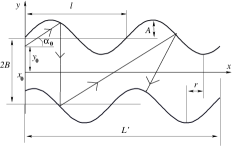
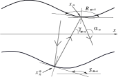
Figure 1: (a) The channel. (b) The parameters used in the map.

We are interested in determining the evolution of $n_{0}$ particles injected on the left side of this channel. The particles are dropped by $N$ sources uniformly distributed along the $y$ axis located at $x=x_{0}$. Each source drops $\frac{n_{0}}{N}$ particles with an angular distribution given by

$$\rho(\alpha_{0})=\frac{n_{0}}{2D(x_{0})}\cos(\alpha_{0}),$$ (2)

where $D(x)=y_{1}(x)-y_{2}(x)$ is the distance between the walls at the $x$-point. We assume that the collisions of the particles with the boundaries are specular.

2.1 The map

In order to find the Poincaré sections corresponding to channels characterized by certain parameters it is necessary to have a discrete map. Since the parameters we shall be using in the next section are such that multiple collisions of the particles with the ripple are improbable. According to our numerical study the occurrence of multiple collisions, for each trajectory is $\sim 10^{-3}$, therefore we may neglect them.

To construct the map let us consider a set of discrete points $(x_{n},\alpha_{n})$ of each particle initially dropped with initial conditions $(x_{0},y_{0},\alpha_{0})$. Here $x_{n}$ is the position in the $x$ direction at the $n$-th collision of the particle with the upper wall and $\alpha_{n}$ is the angle that the trajectory of particle makes with $x$-axis just after the $n$-th collision. The resulting map is

$$\alpha_{n+1}=2\left(S_{n}-R_{n}\right)+\alpha_{n}$$

$$(x_{n+1}-x^{*}_{n})\tan\gamma_{n}+a\sin 2\pi(x^{*}_{n}+r)=2b+a\sin 2\pi x_{n+1}.$$ (3)

From the second line of last equation we see that to express the position of the $(n+1)$-th collision as $x_{n+1}=f(x_{n},\alpha_{n})$, the equation must be solved numerically. The variables $\gamma_{n}$, $R_{n}$, $S_{n}$ and $x^{*}_{n}$ are given by (see Fig. 1 (b)):

$$\gamma_{n}=\pi-\alpha_{n}+2S_{n}$$

$$R_{n}=\tan^{-1}(\frac{dy_{1}}{dx})|_{x_{n}}$$

$$S_{n}=\tan^{-1}(\frac{dy_{2}}{dx})|_{x^{*}_{n}}$$

$$2b+(x^{*}_{n}-x_{n})\tan\alpha_{n}+a\sin 2\pi x_{n}=a\sin 2\pi(x^{*}_{n}+r).$$ (4)

Here $x^{*}_{n}$ stands for position of the particle in the $x$-direction just after the $n$-th collision with the lower wall, $\gamma_{n}$ is the angle that the trajectory of the particle makes with $x$-axis after the $n$-th collision with the lower wall. Finally, $\tan S_{n}$ ($\tan R_{n}$) represents the slope of the line tangent to the lower wall at the point $x=x^{*}_{n}$ (the upper wall at $x=x_{n}$).

We want to indicate for future comparison, that our channel (for $r=\frac{1}{2}$) has the same transmitivity as the semiplane channel with an average width equals to $b$ and the same ripple amplitude. In order to see this, let us consider a particle propagating inside the semiplane channel and other one propagating inside our channel. The trajectory of the particle moving in the semiplane channel defines a succession of collision points ($x^{p}_{n},y^{p}_{n}$) with the upper wall. On the other hand, a particle propagating in our channel, with $r=\frac{1}{2}$ defines a set of collision points with the upper wall ($x_{n},y_{n}$). Because of the specular symmetry respect to the $x$ axis in our channel, the following condition is satisfied

$$(x^{p}_{2n+1},y^{p}_{2n+1})=(x_{n},y_{n}),\qquad n=1,2\dots,$$

if the particles in both channels are dropped with the same initial conditions and the first bounce occurs with the upper wall (if the first bounce is with the lower wall a similar relation is obtained) then it is obtained the same transmitivity in both cases.

3 Poincaré sections

To plot the Poincaréé sections we choose for convenience the conjugate pair ($x_{n}$,$p_{n}$), where $p_{n}=\cos\alpha_{n}$ (see the map in Eq. (3)) is the momentum in the $x$ direction right after the $n$-th collision with the upper wall. In order to have access to all possible orbits with our initial conditions we varied the position of the sources at the $x$ coordinate. For instance, to reach orbits within the islands we placed the sources at the $x$ coordinate of the corresponding fixed point. Notice that we implicitly take a channel of infinite length.

For obtaining the Poincaré plots we set the value $l=1$ and accordingly we have a narrow channel with $b=0.1$ and a wide channel with $b=2.5$. To represent the Poincaré plots, we use the $x$-interval $[0,2]$. We will see that the dynamics of these two channels are quite different. To solve the map in Eq. (3) we use a bisection method applied to $10^{5}$ small intervals along the channel. The numerical code was written in Fortran and the calculations were carried out in a PC with a Pentium IV processor.

For the narrow channel with small ripple amplitudes (e.g $a=0.001$), the system shows a regular dynamics; the corresponding Poincaré plots resemble the phase space of a one dimensional pendulum (see Figs. 2(a) and (b)). This means that the elliptic orbits (an elliptic orbit is an special case of a closed trajectory in the phase space called librational motion [20]) correspond to trapped particles in the channel, moving backward and forward around a stable fixed point.

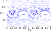
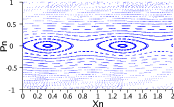
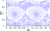
Figure 2: Poincaré plots for the narrow channel. (a) $a=0.001$ and $r=\frac{1}{2}$, (b) $a=0.001$ and $r=\frac{1}{3}$, (c) $a=0.001$ and $r=0$ and (d) $a=0.017$ and $r=\frac{1}{4}$.

The trajectories outside these elliptic orbits represent particles traveling to the left ($p_{n}<0$) or to the right ($p_{n}>0$) of the channel and they never return. We can also see that the position of the fixed points and the size of the region of librational motion depend on the relative phase $r$. For instance, with $r=0$ the elliptic orbits cannot be observed (see Fig. 2 (c)). For other cases the size of the elliptic orbits are clearly remarked. In our case fixed points represent particles bouncing between the same point ($x_{f}$,$p_{f}$) of the upper wall and the point ($x^{*}_{f}$,$p^{*}_{f}$) of the lower wall. The position of fixed points $(x_{f},p_{f})$ can be obtained by considering geometrical arguments (see A).

If we increment $a$ (still for a narrow channel) in some interval (e.g. for the values $r=0.5$, $0<a<0.009$), the dynamics of the system is still regular and the arising librational orbits occupy a larger region. This means that there are more librational orbits accessible to the initial conditions increasing the number of reflected particles in the channel. In the case of $r=0$ and $a=0.01$, the elliptical orbits can now be observed. If we increase $a$ again, the elliptical orbits start to deform, occupying a larger region and the separatrix becomes chaotic with some sizable width (see Fig. 2(d)), this means that more particles can get into the region and they may be reflected. The accessible chaotic region outside the separatrix can not contribute to the reflection because there are some KAM curves that forbid its connection with the separatrix (see Figs. 3 (a) and 2 (d)) . Nevertheless, there is a critical amplitude $a_{c}$ that depends on $r$, for which these KAM curves break allowing the connection of all chaotic regions and then they can contribute to the reflection (see Figs 3 (b), (c) and (d)). For instance for $r=\frac{1}{4}$, $a_{c}=0.015$, for $r=\frac{1}{2}$, $a_{c}=0.027$ and for $r=0$, $a_{c}=0.065$. We observe a principal first-order resonant island surrounded by a chaotic

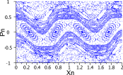
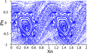
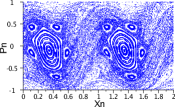
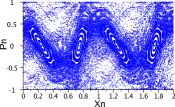
Figure 3: Poincaré plots for the narrow channel. (a) $a=0.04$ and $r=0$, (b) $a=0.032$ and $r=\frac{1}{4}$, (c) $a=0.03$ and $r=\frac{1}{3}$, and (d) $a=0.065$ and $r=0$.

sea, and also a second order resonant islands chain surrounding the first order islands. In Fig. 3 (c) these islands are produced by particles bouncing in the neighborhood of a stable fixed point of period five. If we increase the value of $a_{c}$, more initial conditions get into the chaotic sea due to destruction of regular curves. Notice that the rate at which the KAM curves are destroyed as the amplitude is increased depends on $r$: if we are near to $r=0$ this process is slow and if we are near to $r=\frac{1}{3}$ this process is fast.

In the case of the wide channel, we can see, in contrast to narrow channel, that Poincaré plots for the wide channel show a rather chaotic behaviour, even for small amplitudes (see Fig. 4 (a)), but there are some small regions of librational motion. If the amplitude is increased there exists a critical amplitude for which all KAM curves are destroyed and it produces a global chaos (see Fig 4 (b)). In previous works [18, 21, 22] it has also been observed that the case of global chaos is generally meaningless for applications in waveguides. Due to this behaviour we leave aside the discussion about this type of channel.

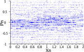
Figure 4: Poincaré plots for the wide channel. (a) $a=0.001$ and $r=\frac{1}{3}$, (b) $a=0.008$ and $r=\frac{1}{3}$.

4 Analytical results for the resistivity

The transmitivity, $T$, is the flux of transmitted particles divided by the incoming flux, as usual the reflectivity is $R=1-T$. For our system it is not possible to have analytical expressions for these quantities. However in some limiting cases we can determine them. In what follows we shall be using a finite channel of length $L=2$.

If we consider a narrow channel ($b\ll L$) with small amplitudes ($a\ll b$) and assume that the ripples are smooth ($a\ll 1$), it is possible to obtain an analytical expression for reflectivity. In this channel, the particles dropped near to the $y$-direction could contribute to reflectivity. In order to obtain an expression for the reflectivity, let us first consider two consecutive collisions, for which the particles collide almost perpendicularly with the walls. Under this assumption we have the following

$$\Delta J\equiv|\sin\alpha_{n}|D(x_{n})-|\sin\gamma_{n-1}|D(x_{n-1}^{*})\approx 0.$$ (5)

In fact, according to Fig.1 (b) and Eq. (4) the relation $\alpha_{n}+\gamma_{n-1}=\pi+2R_{n}$ is fulfilled. For angles such that $\gamma_{n}=\pi/2-\varepsilon$, with $|\varepsilon|\ll 1$, considering the $\Delta x=x_{n}-x_{n-1}^{*}$, taking into account an expansion in Taylor series and keeping terms up to second order in (5) we obtain

$$\Delta J\approx\frac{dD(x)}{dx}\bigg{|}_{x_{n-1}^{*}}\Delta x-2D(x_{n-1}^{*})R_{n}\left(R_{n}+\varepsilon\right).$$ (6)

This equation allows us to corroborate Eq. (5). Notice that $\Delta J=0$ is satisfied trivially for the case of plane walls. Taking into account the conditions of the channel in question, we are free to choose the parameters in such a way that each term in Eq. (6) is too small to be considered. If we now consider the case between two different collisions, for instance the $n$-th and $m$-th collisions we have that

$$|\sin\alpha_{n}|D(x_{n})\approx|\sin\gamma_{m}|D(x_{m}^{*}),$$ (7)

under the same conditions as previously assumed. To see this, notice that the contribution to reflection comes only from particles whose initial conditions reach accessible elliptic orbits, colliding almost perpendicularly with the walls. For this particles the variables $\Delta x$, $\epsilon$ and $R_{n}$ in Eq. (6) can change of sign, in addition, for our conditions the number of collisions is small, and $\Delta J$ is still small.

By using Eqs. (1) and (7), we obtain

$$(2b+a\sin 2\pi x_{n}-\sin 2\pi(x_{n}+r))\cos\beta_{n}$$

$$=(2b+a\sin 2\pi x_{m}-\sin 2\pi(x_{m}+r))\cos\beta_{m},\qquad n\neq m=1,2\ldots$$ (8)

where $\beta_{n}=\frac{\pi}{2}-\alpha_{n}$ is the angle between the velocity and the vertical direction at the $n$-th collision. If we consider particles executing librational motion, $\beta_{n}$ decreases gradually as the particles move forward until they reach a turning point, $x_{N}$, where $\beta_{N}\approx 0$ and then the particle returns. There are two critical angles $\beta_{c1}$ and $\beta_{c2}$, for which the particle does not return. These angles correspond to particles dropped with positive and negative angles, $\alpha_{c1}$ and $-\alpha_{c2}$, respectively (see Fig.1 (a)). The critical angles depend on both the geometrical parameters and the initial position ($x_{0}$,$y_{0}$) at which the particles are dropped. For the parameters involved in the narrow channel, we may assume that $\beta_{c1}\approx\beta_{c2}\equiv\beta_{c}$, and this condition is independent of $y_{0}$ (which is corroborated numerically). To find $\beta_{c}$ we set the point of departure at $(x_{0},y_{0})=(x_{0},y_{1}(x_{0}))$, where $(x_{0},\sin\beta_{c})$ corresponds to an initial point in the phase space that belongs to the largest amplitude of librational motion around at some elliptic fixed point $x=x^{e}_{f0}$. Setting $\beta_{n}=\beta_{c}$, $\beta_{m}=\beta_{N}$, then $x_{n}=x_{0}$ and $x_{m}=x_{N}\approx x^{h}_{f0}$ is close to an hyperbolic fixed point, whose position is determined by $x_{0}$ and Eq. (11). If we substitute these values in Eq. (8) and expand in a Taylor series by dropping terms of order $\left(\frac{a}{b}\right)^{2}$ and keeping terms of order $\beta^{2}_{c}$, we obtain

$$(\beta_{c})^{2} \approx \frac{a}{b}\bigg{[}\sin(2\pi(x^{h}_{f0}+r))+\sin(2\pi x_{0})-\sin(2\pi x^{h}_{f0})$$ (9)

$$- \sin(2\pi(x_{0}+r))\bigg{]},$$

where $x^{h}_{f0}$ is a parameter to be determined. Setting the values $r=\frac{1}{2}$, $x_{0}=\frac{1}{4}$ in the former equation, then $x^{h}_{f0}\approx\frac{3}{4}$ and obtain the value for $(\beta_{c})^{2}\approx\frac{4a}{b}$. This is the same result previously obtained for the semiplane channel [16], but the average width of our channel is twice as large. To find out the general behaviour of $x^{h}_{f0}$ we use the effective potential introduced below.

According to Eq. (7), we have $C=D(x)|\dot{y}|\bigg{|}_{x_{n}}$ with unit speed and $C$ being a constant. Using this condition and the conservation of the energy, it is easy to see that the motion in the $x$-direction is described by [23]:

$${\frac{1}{2}}(\dot{x})^{2}=E-V(x),$$ (10)

with $E$ being the energy of the particle (with unit mass) and $V(x)=\frac{1}{2}|\dot{y}|^{2}$. Hence $V(x_{n})=\left({\frac{C}{D(x)}}\right)^{2}\bigg{|}_{x_{n}}$ can be interpreted as an effective potential at $x_{n}$ that depends only on the geometric parameters of the channel. The usefulness of this effective potential relies on the fact that it explains the regular motion and allows one to find out the $x$-position and the stability of the fixed points.

If we use the profiles described by Eq. (1), then $D(x)=2b+a\sin 2\pi x-a\sin 2\pi\left(x+r\right)$ and the potential takes the form of an oscillatory periodic function. This explains why Poincaré plots resemble the phase space of a simple pendulum. An interesting case is for $r=0$, where $V(x)$ is constant and consequently, within the approximation used, there are not trapped particles. This explains the behaviour of almost straight lines trajectories shown in Fig. 2 (c). This situation occurs approximately in a flat channel. We can find the $x$ position of the fixed point by obtaining the maxima and minima of $V(x)$ which represent the elliptic fixed points $x_{f}^{e}$ and the hyperbolic fixed points $x_{f}^{h}$ respectively. We obtain that the fixed points satisfy the condition:

$$\cos 2\pi x_{f}=\cos 2\pi(x_{f}+r).$$ (11)

It is easy to see, for instance, that for $r=1/2$, the elliptic and hyperbolic fixed points are located respectively in $x^{e}_{f}=\frac{1}{4}\pm n$ and $x^{h}_{f}=\frac{3}{4}\pm n$, with $n$ an integer; and that for the case of $r=\frac{1}{4}$, the elliptic and hyperbolic fixed points are located respectively at $x^{e}_{f}=\frac{3}{8}\pm n$ and $x^{h}_{f}=\frac{7}{8}\pm n$. Let us mention that an elliptic fixed point and the consecutive hyperbolic point are separated by a distance $d_{s}=1/2$ except for $r=0$ where $d_{s}=1/4$. These results are in agreement with the Poincaré plots obtained in the previous section.

Taking into account the previous results, we see that the transmitivity takes the form:

$$T=\frac{\int_{-\alpha_{c}}^{\alpha_{c}}\rho(\alpha_{0})\cos\alpha_{0}d\alpha_{0}}{\int_{-\frac{\pi}{2}}^{\frac{\pi}{2}}\rho(\alpha_{0})\cos\alpha_{0}d\alpha_{0}}=1-\frac{2\int_{0}^{\beta_{c}}\,\sin\beta_{0}\rho(\frac{\pi}{2}-\beta_{0})d\beta_{0}}{\int_{-\frac{\pi}{2}}^{\frac{\pi}{2}}\rho(\alpha_{0})\cos\alpha_{0}d\alpha_{0}},$$ (12)

where $\alpha_{0}=\frac{\pi}{2}-\beta_{0}$. Using Eq. (9) and assuming $\beta_{0}$ small, we obtain

$$R\approx\frac{4}{3\pi}\beta_{c}^{3}=G(r)a^{3/2},$$ (13)

where $G(r)$ is given by

$$G(r) = \frac{4}{3\pi\,b^{3/2}}\left[\sin(2\pi(x^{h}_{f}+r))+\sin(2\pi x_{0})\right.$$ (14)

$$-\left.\sin(2\pi x^{h}_{f})-\sin(2\pi(x_{0}+r))\right]^{3/2}.$$

In the former $x^{h}_{f}=x^{h}_{f}(r)$ is determined from the positions of the sources at $x_{0}$ and from Eq. (11). Let us emphasize that the length $L$ of our channel is bigger than the distance between two consecutive hyperbolic fixed points, this makes the function $G$ independent of $L$. In fact, particles executing librational motion cannot escape from the channel at the right side. Otherwise, in general, $G$ is $L$-dependent. In Fig. 5 we show a graph of reflectivity given by Eq. (13). The important point here is that we can choose the parameter $r$ to obtain a required reflectivity, for instance for $r=0.67$ we have that the reflectivity is maximal.

The resistivity $\rho$ of the channel is an important measurable quantity that is related to reflectivity through Landauer’s formula [24]:

$$\rho\propto\frac{R}{T},$$ (15)

which is of great importance in condensate matter and it can be calculated from a single particle theory with no dissipation [25]. From Eqs. (13) and (15) we conclude that the resistivity, for the narrow channel, is:

$$\rho\propto G(r)a^{\frac{3}{2}}.$$ (16)

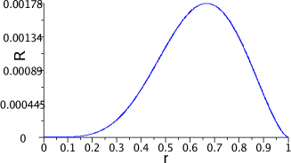
Figure 5: Reflectivity of the narrow channel as a function of $r$, for the value $a=0.001$ and $x_{0}=0$.

Let us now briefly discuss the case of the wide channel with small amplitudes. According to Eq. [16] chaotic scattering on surfaces with deterministic profiles is practically indistinguishable from the scattering on surfaces with random profiles. It is known that the classical resistivity $\rho$ of a plate with rough surfaces grows quadratically [2, 3] with the root mean square (rms) height of the roughness $\xi$, when $\xi<<2b$. By using Landauer’s formula, we can express the transmitivity as:

$$T(\xi)=1-c\xi^{2},$$ (17)

where $c$ is a constant that depends on the geometrical properties of the channel. Assuming that the rms height of the effective random profile is proportional to the amplitudes of the ripples $a$, we conclude that

$$R=F(r,L)a^{2},$$ (18)

and hence $\rho\propto F(r,L)a^{2}$. In contrast to the narrow channel, the function $F(r,L)$ remains unknown.

5 Numerical results for the reflectivity and transmitivity

To obtain numerical results we considered $N=10^{2}$ sources at $x_{0}=0$ and $n_{0}=10^{5}$, with the distribution given by Eq. (2). Our numerical method takes into account the possibility of multiple collisions, by generalizing the map in Eq. (3)

In order to check the confidence of our numerical method, first in Fig. 6 we show the numerical results ($|\log R|$ vs. $|\log a|$) with cross symbols and the corresponding linear fit in solid line for different values of $r$ and small amplitudes. In Figs. 6 (a) and (b), for the narrow channel, the fitting gives the results $R\sim a^{1.59}$ for $r=\frac{1}{4}$ and $R\sim a^{1.58}$ for $r=\frac{1}{3}$. While for the wide channel we have $R\sim a^{1.9}$ for $r=\frac{1}{2}$ and $R\sim a^{2.15}$ for $r=0$. The corresponding theoretical results are $R\sim a^{1.5}$ for Figs. 6 (a) and (b), and $R\sim a^{2}$ for Figs. 6 (c) and (d). According to these results the agreement with the analytical results in Eqs. (13) and (18) is good. On the other hand, we calculate the error, $E=\sqrt{\sum_{i}(R_{i}^{th}-R_{i}^{num})^{2}}$, where $R_{i}^{th}$ are determined from Eq. (13) and $R_{i}^{num}$ are the numerical results using in Figs. 6 (a) and (b). We obtain that $E=6.8\times 10^{-5}$ for $r=1/4$ and $E=1.5\times 10^{-4}$ for $r=1/3$, which are small. Second, in Fig. 7 we show the transmitivity for a narrow channel for $r=1/2$. We compare this result with the Fig. 4 (c) presented in Ref. [16] and observe a good agreement.

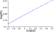
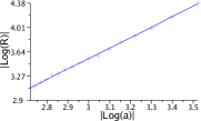
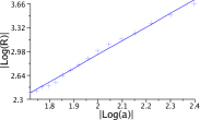
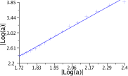
Figure 6: Numerical results of $|\log R|$ vs. $|\log a|$ for the narrow channel (Figs. (a) and (b)). and for the wide channel (Figs. (c) and (d)). In (a) $r=\frac{1}{4}$, in (b) $r=\frac{1}{3}$, in (c) $r=\frac{1}{2}$, and finally in (d) $r=0$.

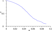
Figure 7: Numerical results for the transmitivity in the narrow channel for $r=1/2$.

It is known that a cavity based on the narrow channel has potential applications to chaotic waveguides and microlasers [19]. For these applications it is important to have a big number of trapped particles (rays) which give a high reflectivity. Our channel is an example of this kind of systems. As already mentioned we introduced a phase shift, $r$, as a new parameter which makes the dynamics of these kind of channels more interesting. To see this we varied $r$ and observed a considerable increment of the resistivity comparing with the semiplane channel, which is equivalent to our channel whenever $r=1/2$.

In Fig. 8 we show a plot for the reflectivity as a function of the phase shift, for different amplitudes of the ripple. In this figure we indicate reference points at each curve located at $r=0.5$ which define the $R_{ref}$. At these points, we observe that the resistivity is maximal for values of $r\neq 0.5$, consequently the resistivity of the channel can be manipulated by varying the phase shift. If we define $R_{max}$ as the maximum value of the reflectivity for a given $a$, we can introduce a parameter, $I$, that measures the relative increment of the reflectivity.

$$I=\left|\frac{R_{max}-R_{ref}}{R_{ref}}\right|,$$ (19)

The values of $I$ for the curves $A$, $B$, $C$ and $D$ are $0.009$, $0.087$, $0.230$, and $0.400$ respectively, which represent increase of $0.9\%$, $8.7\%$, $23\%$ and $40\%$. Let us observe that bigger values of $I$ result from smaller values of the amplitude (see curves $C$ and $D$ in Fig.8). This result can be explained by observing that the rate of destruction of the librational orbits, as $a$ is increased, is slower for $r=1/2$ than for other cases. For the curves $C$ and $D$ in Fig.8 the main contribution to the reflectivity comes from particles executing librational motion. To illustrate this see Fig.3 (c), from which we can see large regular regions corresponding to this kind of particles.

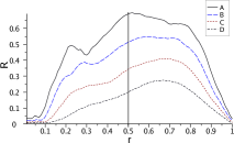
Figure 8: Reflectivity of the narrow channel vs phase for (A) $a=0.06$; (B)$a=0.05$; (C)$a=0.04$; (D)$a=0.03$

6 Concluding remarks

We have studied some of the transport properties of classical particles through a two-dimensional channel with sinusoidal boundaries in the ballistic regime. We restrict ourselves to cases of narrow channels and wide channels. In the first one, Poincaré plots show a regular dynamics for small amplitudes. A transition to mixed chaos is observed as the amplitude is increased. In the second case, chaotic behaviour appears even for small amplitudes. For bigger amplitudes global chaos is reached. In both cases the rate of the transition to chaos depended on the phase shift. For the narrow channel, the contributions of regular and chaotic regions to reflection were identified via Poincaré plots.

An analytical approximate expression for the classical resistivity taking into account small ripple amplitudes was obtained. We found, that the resistivity $\rho$ behave like $\rho(a,r)\propto G(r)a^{\frac{3}{2}}$ in the case of narrow channel (showing a regular dynamics) and for wide channel (showing a chaotic dynamics) $\rho(a,r,L)\propto F(r,L)a^{2}$, where $G(r)$ being a known function while $F(r,L)$ remains unknown. These results were corroborated by numerical calculations.

Taking as parameters the amplitude of the ripples and the phase shift between the boundaries, we observed that the manipulation of the phase shift results in a considerable increment of the resistivity when it is compared with that obtained in the semiplane channel. This shows that the use of the phase shift allows favorable conditions for potential applications in waveguides and resonators. For this applications a complementary quantum analysis is necessary.

Appendix A

In order to find the localization of the fixed points we refer to Fig. 9 taking the case in which the upper and lower walls are in phase $r=0$, see Eq. (1). The fixed points represent particles bouncing between the same points with the upper and lower rippled boundaries respectively: $(x_{f},y_{1}(x_{f}))$ and $(x_{f}^{*},y_{2}(x_{f}^{*}))$. In order to find these points we must first find the points on the walls fulfilling the condition $\frac{dy_{1}}{dx}\mid_{x_{f}}=\frac{dy_{2}}{dx}\mid_{x_{f}^{*},r=0}$, this leads to:

$$\cos(2\pi x_{f}) = \cos(2\pi(x_{f}+h)),$$ (20)

where for convenience we write $x_{f}^{*}=x_{f}+h$.

Let us consider two parallel lines $N$ and $N_{1}$. These lines intercept the curves $y_{1}$ and $y_{2}$ at the points $(x_{f},y_{1}(x_{f}))$ and $(x_{f}^{*},y_{2}(x_{f}^{*}))$. They are normal to the upper wall and lower wall at the points to the tangents $T$ and $T_{1}$ at $x_{f}$ and $x_{f}^{*}$ respectively. If $x_{f}$ is the $x$ position of a fixed point then $N$ and $N_{1}$ must be equal once we have made an horizontal shift between the walls by a quantity $r$ in our initial configuration (see Fig. 9). To find $r$, we must obtain the $x$ coordinate of the point $c$ ($x_{c}$) that is defined by the intercept between the lines $N$ and $H=y_{2}\mid_{x_{f}^{*}}$. Consequently $r$ is determined by:

$$r=x_{f}^{*}-x_{c}.$$ (21)

This leads to the condition for $r$

$$r=h-4\pi ba\cos(2\pi x_{f})+2\pi a^{2}\cos 2\pi x_{f}(\,{\rm sin}\,2\pi(x_{f}+h)-\,{\rm sin}\,2\pi x_{f}),$$ (22)

where $h$ is given by Eq. (20). Finally the $x$ component of the momentum for fixed points is given by:

$$p_{f}=\cos\left(\tan^{-1}\left(-\frac{1}{\frac{dy_{1}}{dx}|_{x_{f}}}\right)\right).$$ (23)

We can obtain the same result as the previously obtained through the method of the effective potential given in Eq. (11) by considering small amplitudes of the rippled in Eqs. (20) and (22).

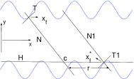
Figure 9: The channel for $r=0$.

References

- [1] Y. Alhassid, Rev. Mod. Phys. 72 (2000) 895.
- [2] N. Trevedi, N. W. Ashcroft, Phys. Rev. B38 (1988) 12298.
- [3] A. E. Meyerovich, S. Stepaniats, Phys. Rev. B51 (1995) 17116.
- [4] C. M. Marcus, A. J. Rimberg, R. M. Westerbelt, P. F. Hopkins and A. D. Gossard, Phys. Rev. Lett. 69 (1992) 506.
- [5] L. A. Bunimovich, Funct. Anal. Appl. 8 (1974) 254.
- [6] Y. G. Sinai, Russ. Math. Surv. 25 (1970) 137.
- [7] M. J. Berry, J. A. Katine, R. M. Westervelt and A. C. Gossard, Phys. Rev. B50 (1994) 17721.
- [8] J. Burki, R. E. Goldstein, and C. A. Stafford, Phys. Rev. Lett. 91 (2003) 254501.
- [9] K. Nakamura and T. Harayama, Quantum chaos and quantum dots, (Oxford) (2004).
- [10] L. P. Kouwenhoven et. al., Phys. Rev. Lett. 65 (1990) 361.
- [11] D. P. Sanders, H. Larralde Phys. Rev. E 73 (2006) 026205.
- [12] L. Baowen, G. Casati, and J. Wang Phys. Rev. E 67 (2003) 021204.
- [13] G. Casati, T. Prosen Phys. Rev. Lett. 83 (1999) 4729.
- [14] D. Alonso, A. Ruiz, and I. de Vega Phys. Rev. E 66 (2002) 066131.
- [15] O. G. Jepps and L. Rondoni J. Phys. A: Math. Gen. 39 (2006) 1311.
- [16] G. A. Luna-Acosta, A. Krokhin, M. A. Rodriguez, and P. H. Hernández-Tejeda Phys. Rev. B54 (1996) 11410.
- [17] G. A. Luna-Acosta, K. Na, L. E. Reichl, and A. Krokhin Phys. Rev. E53 (1996) 3271.
- [18] J. A. Méndez-Bermúdez, G.A. Luna Acosta, P.eba, and K. N. Pichugin Phys. Rev. B67 (2003) 161104.
- [19] O. Bendix, J. A. Méndez-Bermúdez, G. A. Luna-Acosta, U. Kuhl, and H-J Stöckmann Microelectronics Journal 36 (2005) 285.
- [20] H. Goldstein, C. Poole and J. Safko Classical mechanics (Addison Wesley) (2002).
- [21] C. Gmachl, F. Capasso, E. E. Narimanov, J. U. Nöckel, A. D. Stone, J. Faist, D. L. Sivco, and A. Y. Cho Science 280 (1998) 1556.
- [22] J. A. Méndez-Bermúdez, G. A. Luna-Acosta, P. Seba, and K. N. Pichugin Phys. Rev. E 66 (2002) 046207.
- [23] I. Percival and D. Richards Introduction to dynamics (Cambridge University Press) (1982).
- [24] R. Landauer IBM J. Res. Dev. 1 (1957) 223.
- [25] M. P. Das and F. Green J. Phys.: Condens. Matter 15 (2003) L687.