A framework for protein and membrane interactions

Abstract

We introduce the Bio$\beta$ Framework, a meta-model for both protein-level and membrane-level interactions of living cells. This formalism aims to provide a formal setting where to encode, compare and merge models at different abstraction levels; in particular, higher-level (e.g. membrane) activities can be given a formal biological justification in terms of low-level (i.e., protein) interactions.

A Bio$\beta$ specification provides a protein signature together a set of protein reactions, in the spirit of the $\kappa$-calculus. Moreover, the specification describes when a protein configuration triggers one of the only two membrane interaction allowed, that is “pinch” and “fuse”.

In this paper we define the syntax and semantics of Bio$\beta$, analyse its properties, give it an interpretation as biobigraphical reactive systems, and discuss its expressivity by comparing with $\kappa$-calculus and modelling significant examples.

Notably, Bio$\beta$ has been designed after a bigraphical metamodel for the same purposes. Hence, each instance of the calculus corresponds to a bigraphical reactive system, and vice versa (almost). Therefore, we can inherith the rich theory of bigraphs, such as the automatic construction of labelled transition systems and behavioural congruences.

1 Introduction

Cardelli in [5] has convincingly argued that the various biochemical toolkits identified by biologists can be described as a hierarchy of abstract machines, each of which can be modelled using methods and techniques from concurrency theory. Like other complex situations, it seems unlikely to find a single notation covering all aspects of a whole organism; instead, several models, often presented as process calculi, have been proposed in literature, each focusing on specific aspects of the biological system, at different levels of abstractions. This arises the problem of how to integrate these models. Indeed, these machines operate in concert and are highly interdependent: “to understand the functioning of a cell, one must understand also how the various machines interact” [5]. To this end, we need a general metamodel, that is, a framework, where these models (possibly at different abstraction levels) can be encoded, and their interactions can be formally described. Eventually “we will need a single notation in which to describe all machines, so that a whole organism can be described” [5].

As a step towards this long-term goal, in this paper we present Bio$\beta$, a framework calculus for dealing with both protein-level and membrane-level interactions. Many specific models, with protein interactions and membrane trafficking, can be encoded in Bio$\beta$ by providing a specification. Notably, different specifications can be merged, which corresponds to “put together” different models and systems, often at different levels of abstraction. This allows to investigate the interactions between these models, which otherwise would be kept separate; for instance, this allows to foresee emerging properties, such as behaviours due to interactions of different abstraction levels, and which cannot be observed within a single machine model due to its intrinsic abstractions.

A fundamental design choice is that this framework has to be biologically sound, i.e., it must admit only systems and reactions which are biologically meaningful, especially at lower level machines (i.e. protein). This is important because in this way, encoding a given model in the framework provides automatically a formal, biologically sound justification for the model (or “implementation”) in terms of protein reactions and explains how its membrane-level interactions are realised by protein machinery. Also, the representation of a specific model is less error-prone.

To this end, Bio$\beta$ has been designed after a bigraphical metamodel, called biobigraphs and biological bigraphical reactive systems (BioRS) and presented in a companion paper [3], for dealing with both protein-level and membrane-level interactions. Actually, Bio$\beta$ can be seen as a syntactic formalism for representing precisely biobigraphical reactive systems. However, for sake of simplicity and lack of space, in this paper we will not discuss the connection between Bio$\beta$ and biobigraphs, which will be presented in forthcoming work. For the purposes of the present paper, it suffices to know that biobigraphs, and hence Bio$\beta$, are adequate with respect to Danos and Laneve’s $\kappa$-calculus, one of the most accepted formal model of protein systems: we can describe all and only protein configurations and interactions of the $\kappa$-calculus. (Is important to notice, however, that our methodology is general, and can be applied to other formal protein models.) Hence, the Bio$\beta$ Framework can be seen somehow as an extension of the $\kappa$-calculus, adding biological compartments (that is membranes); however, this is a consequence of the fact that the underlying model, the biobigraphs, are adequate w.r.t. the $\kappa$-calculus.

When membranes come into play one wants to deal also with membrane transport, hence, we have to take into consideration reactions like endocytosis, exocytosis, cellular fusion and vesiculation. Actually, as observed by biologists (see [1] and [2, Ch. 15]), membrane interactions present always a “preparation phase”, where some proteins (receptors and ligands) interact to get in place, followed by the actual “membrane reconfiguration” phase, which can be either a pinch or a fuse [6]. Therefore, biobigraphs, and Bio$\beta$, provide just two general rules for all membrane interactions, whilst the preparation phase depends on the specific proteins involved and hence left to the encoding of the specific model.

Summarizing, for encoding a given model one has just to instantiate this general schema by specifying (a) a protein signature, that is a set of abstract proteins; (b) a set of protein rules, describing protein interactions ignoring compartments; (c) a set of protein configurations which trigger a mobility reaction. Then, all other reactions (mobility, in particular) are automatically provided by the framework, in a sound way. Hence, modelers can focus on protein-level aspects, leaving to the framework the burden to deal with biological compartments and membrane transport.

A further motivation for our framework comes from the many general results provided by bigraphs. We mention here only the construction of compositional bisimilarities [10], allowing to prove that two systems are observational equivalent, that is, they can be exchanged in any organism without that the overall behaviour will change. Also for this application it is important to restrict the systems allowed by the framework to only those biologically meaningful.

Synopsis

In Section 2 we present the Bio$\beta$ framework: its syntax, a type system for characterizing well-formed (i.e., biologically meaningful) terms, and general operational semantics. As an example application of this framework, in Section 3 we model the mechanism of membrane traffic. In Section 4 we provide a formal connection between $\kappa$-calculus and Bio$\beta$. Related work is discussed in Section 5, and in Section 6 we draw some conclusion and plan future work.

2 The Bio$\beta$ Framework

In this section we present the Bio$\beta$ framework. Although one should not think of Bio$\beta$ necessarily as an extension of the $\kappa$-calculus, its connections with that model are quite strong, and hence it is convenient to reuse notations and concepts from $\kappa$.

2.1 Syntax

The language of the Bio$\beta$ framework is parametric over a protein signature $(\mathcal{P}=\mathcal{P}_{p}\cup\mathcal{P}_{ap},s:\mathcal{P}\to\mathbb{N})$, where $\mathcal{P}$ is a finite set of (abstract) proteins, partitioned into polar $\mathcal{P}_{p}$ and polar $\mathcal{P}_{ap}$. $\mathcal{N}$ is an enumerable set of edge names, and $s\colon\mathcal{P}\to\mathbb{N}$ assigns to every protein the number of its domain sites.

A (protein) interface is a map from $\mathbb{N}$ to $\mathcal{N}+\{h,v\}$ (ranged over $\rho$, $\sigma$, $\ldots$). Given an interface $\rho$ and a protein name $A\in\mathcal{P}$, a site $(A,i)$ is visible if $\rho(i)=v$, hidden if $\rho(i)=h$, and tied if $\rho(i)\in\mathcal{N}$. A site is free if it is visible or hidden. In the following, we will write $\rho=1+\bar{2}+3^{x}$ to mean $\rho(1)=v$, $\rho(2)=h$, and $\rho(3)=x$. Denote with $|\rho,x|$ the number of occurrences of $x$ in $\rho$, that is, $|\rho,x|\triangleq|\{i\in s(\rho)\mid\rho(i)=x\}|$.

The syntax of Bio$\beta$ over a given protein signature, consists of systems, which can be nested, and membranes. Polar proteins can freely float at the level of systems, while apolar proteins can be embedded into membranes. Let $A_{t}\in\mathcal{P}_{t}$, for $t\in\{p,ap\}$, $n\in\mathcal{N}$, and $\rho\colon\mathbb{N}\to\mathcal{N}+\{h,v\}$ be a protein interface.

$$P,Q ::=\diamond\mid A_{p}(\rho)\mid\Lbag S\lbag P\rbag\Rbag\mid P\ast Q\mid\nu n.P\mid\mathsf{p}_{n}\fatsemi P\mid\mathsf{f}_{n}\fatsemi\Lbag S\lbag P\rbag\Rbag$$ (Systems)

$$S,T ::=\mathbf{0}\mid A_{ap}(\rho)\mid S\star T\mid\mathsf{p}^{\perp}_{n}\fatsemi S\mid\mathsf{f}^{\perp}_{n}$$ (Membranes)

Systems are polar solutions (soluble in aqueous environments), which can be either the empty system $\diamond$, or a polar protein $A_{p}(\rho)$, or a compartment $\Lbag S\lbag P\rbag\Rbag$, or a group of systems $P\ast Q$, or a system prefixed by a new name constructor $\nu n.P$. Membranes are apolar solutions (soluble in oily environments), which can be the empty membrane $\mathbf{0}$, or an apolar protein $A_{ap}(\rho)$, or a group of apolar solutions $S\star T$. Notice that membranes are not sequences of actions (as, e.g., in Brane calculus [4]) but simply a collection of proteins. As usual the “new” operator is a binder: in $\nu n.P$, $P$ is the scope of the binder $\nu n$. Sharing of names on interfaces represent protein domain-domain bonds. For instance $(x)(A(1^{x})\mathbin{,}B(1+2^{x})))$ is a protein solution where there is a bond between sites $(A,1)$ and $(B,2)$.

Figure 1: Vesiculation and endocytosis can be generalized by means of an inward and outward pinch, and fusion and exocytosis by a horizontal and vertical fuse, respectively.

Finally, the special constructors pinch $\mathsf{p}$ and fuse $\mathsf{f}$, together with their co-actions $\mathsf{p}^{\perp},\mathsf{f}^{\perp}$, to represent when a compartment reconfiguration takes place. These actions are inspired by the two basic membrane reconfiguration processes, namely “pinch” and “fuse”. A membrane can be pinched (either outward or inward, Figure 1 left), forming a bubble that detaches producing a new compartment; or two membranes can fuse, in either directions (Figure 1 right) mixing contents. Intuitively, $\mathsf{p}_{n}\fatsemi P$ can be seen as a system $P$ waiting to complete, or commit, a pinch interaction with another system featuring the co-action $\mathsf{p}_{n}^{\perp}$; similarly for $\mathsf{f}$. Thus, these actions are prefixes which freeze the continuation system/membrane until the compartment reconfiguration is completed. The subscripts pair-up corresponding actions and co-actions.

Let us define the co-action operator $(\cdot)^{\perp}$ mapping each mobility action to its dual, and such that $((\cdot)^{\perp})^{\perp}=id$; this operator is extended to sets of actions as $S^{\perp}\triangleq\{s^{\perp}\mid s\in S\}$. Moreover, for a set of names $X\subseteq\mathcal{N}$, the restriction of a set of actions over $X$ is $S{\upharpoonright}_{X}\triangleq\{s_{x}\in S\mid x\in X\}$. In the following, $P,Q,R,\ldots$ range over systems, $S,T,\ldots$ over membranes and $K,L,H,\ldots$ over both systems or membranes.

The set of free names $fn(P)$ and $fn(S)$ are defined as usual, covering also subscripted names on mobility actions (clearly restriction on names binds also action names). In the following $fn(K_{1},\dots,K_{n})$ stands for $\bigcup_{i=1}^{n}fn(K_{i})$, for every $K_{i}$ either a system or a membrane.

Let $\textsc{Act}\triangleq\{\mathsf{p}_{n},\mathsf{p}^{\perp}_{n},\mathsf{f}_{n},\mathsf{f}^{\perp}_{n}\mid n\in\mathcal{N}\}$ be the set of all mobility actions. We define the sets of occurring actions $act(P)$, $act(S)\subseteq\textsc{Act}$ on systems and membranes, respectively, as follows:

$$act(\diamond)=act(A_{p}(\rho))=\emptyset\qquad act(\Lbag S\lbag P\rbag\Rbag)=act(S)\cup act(P)\qquad act(P\ast Q)=act(P)\cup act(Q)$$

$$act(\mathbf{0})=act(A_{ap}(\rho))=\emptyset\qquad act(\nu n.P)=act(P)\qquad act(S\star T)=act(S)\cup act(T)$$

$$act(\mathsf{p}_{n}\fatsemi P)=\{\mathsf{p}_{n}\}\cup act(P)\quad act(\mathsf{f}_{n}\fatsemi P)=\{\mathsf{f}_{n}\}\cup act(P)\quad act(\mathsf{p}^{\perp}_{n}\fatsemi S)=\{\mathsf{p}^{\perp}_{n}\}\cup act(S)\quad act(\mathsf{f}^{\perp}_{n})=\{\mathsf{f}^{\perp}_{n}\}$$

Bio$\beta$ terms can be rearranged according to a structural equivalence $\equiv$, defined to be the least equivalence closed under $\alpha$-equivalence and satisfying the rules below:

$$\begin{array}[]{c@{\qquad}c@{\qquad}c@{\qquad}c}\displaystyle\frac{}{P\ast\diamond\equiv P}&\displaystyle\frac{}{S\star\mathbf{0}\equiv S}&\displaystyle\frac{\mathsf{op}\in\{\ast,\star\}}{K\mathbin{\mathsf{op}}L\equiv L\mathbin{\mathsf{op}}K}&\displaystyle\frac{\mathsf{op}\in\{\ast,\star\}}{K\mathbin{\mathsf{op}}(L\mathbin{\mathsf{op}}H)\equiv(K\mathbin{\mathsf{op}}L)\mathbin{\mathsf{op}}H}\end{array}$$

$$\begin{array}[]{c@{\qquad}c@{\qquad}c@{\qquad}c}\displaystyle\frac{n\neq m}{\nu n.\nu m.P\equiv\nu m.\nu n.P}&\displaystyle\frac{}{\nu n.\diamond\equiv\diamond}&\displaystyle\frac{n\notin fn(Q)}{\nu n.(P\ast Q)\equiv(\nu n.P)\ast Q}&\displaystyle\frac{n\notin fn(S)}{\nu n.\Lbag S\lbag P\rbag\Rbag\equiv\Lbag S\lbag\nu n.P\rbag\Rbag}\end{array}$$

$$\begin{array}[]{c@{\qquad}c@{\qquad}c@{\qquad}c@{\qquad}c}\displaystyle\frac{\mathsf{op}\in\{\ast,\star\}\quad K\equiv L}{K\mathbin{\mathsf{op}}H\equiv L\mathbin{\mathsf{op}}H}&\displaystyle\frac{P\equiv Q\quad S\equiv T}{\Lbag S\lbag P\rbag\Rbag\equiv\Lbag T\lbag Q\rbag\Rbag}&\displaystyle\frac{t\in\{\mathsf{p},\mathsf{p}^{\perp},\mathsf{f}\}\quad K\equiv L}{t_{n}\fatsemi K\equiv t_{n}\fatsemi L}&\displaystyle\frac{t\in\{\mathsf{p},\mathsf{f}\}\quad n\neq m}{\nu n.(t_{m}\fatsemi P)\equiv t_{m}\fatsemi\nu n.P}\end{array}$$

Well-formedness

As for other languages for graph-like structures, the syntax above is too general, since many syntactically correct terms do not have a clear biological meaning. In this subsection give an informal description of the well-formedness conditions that terms must satisfy; in the next subsection we will present a type system enforcing these conditions.

Unsurprisingly, these conditions are similar to those of related models, such as the $\kappa$-calculus, since they are motivated by biochemical properties of proteins and membranes.

First, protein bonds can form only between exactly two active sites on protein surfaces. Hence, terms like $(x)(A(1^{x}))$ or $(x)(A(1^{x})\mathbin{,}A(1^{x})\mathbin{,}B(1^{x}))$ have to be discarded. This requirement is extended to action names, because we want to pair-up just a couple of actions at once. Furthermore, a pinch action can be connected only to co-pinch, and similarly for fuse and co-fuse.

Regarding membranes, we have to ensure the impermeability of membrane boundaries: complexations cannot take place through membranes, hence protein bonds cannot cross them. Thus, terms like $A(1^{x})\ast\Lbag\mathbf{0}\lbag B(1^{x})\rbag\Rbag$ have to be ruled out.

Another (more technical) condition is that continuations after mobility actions cannot have other actions. The intuition is that a membrane engaged with a pinch or fuse interaction, has to complete it before initiating another one.

We summarize these conditions in the follwing definition.

Definition 2.1 (Well-formedness).

A system $P$ is well-formed if the following conditions hold:

Graph-likeness:

free names occurs at most twice in $P$, and every binder ties either 0 or 2 occurrences;

Impermeability:

for any occurrence of a compartment $\Lbag S\lbag Q\rbag\Rbag$ in $P$, $fn(Q)\subseteq fn(S)$ hold;

Action pairing:

for any occurrence of an action $t_{n}$ ($t\in\{\mathsf{p},\mathsf{f}\}$), the name $n$ can appear only in the co-action $t_{n}^{\perp}$.

Action prefix:

for any occurrence of a prefix $t_{n}\fatsemi Q$ $(t\in\{\mathsf{p},\mathsf{p}^{\perp},\mathsf{f}\})$ in $P$, $act(Q)=\emptyset$ hold.

As expected, well-formedness is preserved by structural equivalence:

Proposition 2.1 (Well-formedness is up to $\equiv$).

Let $P$, $Q$ systems s.t. $P\equiv Q$, $P$ is well-formed if it is $Q$.

2.2 Type system

In this subsection we present a type system for Bio$\beta$ terms, which provides a formal procedure for checking well-formedness. As usual in type theory, terms are typed by judgements w.r.t. some environment.

Definition 2.2 (Judgement).

A type $\tau\subseteq\textsc{Act}$ is a finite set of mobility actions.

A judgement for a Bio$\beta$ term $K$ (a system or a membrane) is of the form $\Gamma_{1};\Gamma_{2}\vdash K:\tau$, where the environment $\Gamma_{1};\Gamma_{2}$ is formed by two sets of names, such that $\Gamma_{1}\cap\Gamma_{2}=\emptyset$, each of which is written as a list of the form $x_{0},\dots,x_{n}$.

The two sets in the environment keep track of the free names in terms, and the number of times each name occurs: in our case, if $n\in\Gamma_{1}$ it occurs once, if $n\in\Gamma_{2}$ then it occurs twice. Types keep track of mobility actions/co-actions occurring with free names.

Moreover, let $\mathsf{ok}_{e}$ and $\mathsf{ok}_{t}$ be two predicates defined as follows:

$$\mathsf{ok}_{e}(\Gamma_{1},\Gamma_{2},\Delta_{1},\Delta_{2})\stackrel{{\scriptstyle\triangle}}{{\iff}}(\Gamma_{1}\cup\Gamma_{2})\cap(\Delta_{1}\cup\Delta_{2})=\emptyset\qquad\qquad\mathsf{ok}_{t}(\Gamma,\tau,\sigma)\stackrel{{\scriptstyle\triangle}}{{\iff}}(\tau{\upharpoonright}_{\Gamma})^{\perp}=\sigma{\upharpoonright}_{\Gamma}$$

The first predicate checks if two environments share no names. The second predicate checks if the two types $\tau$, $\sigma$ pair-up correctly, i.e., they create correct actions-coactions pairs using names in $\Gamma$.

$$(\textsf{empty})\ \frac{\displaystyle\epsilon\in\{\mathbf{0},\diamond\}}{\displaystyle\emptyset;\emptyset\vdash\epsilon:\emptyset}\qquad\qquad\frac{\displaystyle A\in\mathcal{P}\quad\forall x\in fn(\rho).\ |\rho,x|\leq 2}{\displaystyle\{x\in fn(\rho)\mid|\rho,x|=1\};\{x\in fn(\rho)\mid|\rho,x|=2\}\vdash A(\rho):\emptyset}\ (\textsf{prot})$$

$$(\textsf{action})\ \frac{\displaystyle t\in\{\mathsf{p},\mathsf{p}^{\perp},\mathsf{f}\}\quad\Gamma_{1};\Gamma_{2}\vdash K:\emptyset\quad act(K)=\emptyset}{\displaystyle\Gamma_{1},x;\Gamma_{2}\vdash t_{x}\fatsemi K:\{t_{x}\}}\qquad\quad\frac{\displaystyle\Gamma_{1};\Gamma_{2}\vdash P:\tau\quad x\notin\Gamma_{1}\quad\tau{\upharpoonright}_{\{x\}}=\emptyset}{\displaystyle\Gamma_{1};\Gamma_{2}\setminus\{x\}\vdash\nu x.P:\tau}\ (\nu\textsf{-prot})$$

$$(\textsf{co-f})\ \frac{\displaystyle}{\displaystyle x;\emptyset\vdash\mathsf{f}^{\perp}_{x}:\{\mathsf{f}^{\perp}_{x}\}}\qquad\qquad\frac{\displaystyle t\in\{\mathsf{p},\mathsf{f}\}\quad\Gamma_{1};\Gamma_{2},x\vdash P:\tau\cup\{t_{x},t_{x}^{\perp}\}\quad\{t_{x},t_{x}^{\perp}\}\cap\tau=\emptyset}{\displaystyle\Gamma_{1};\Gamma_{2}\vdash\nu x.P:\tau}\ (\nu\textsf{-action})$$

$$(\textsf{par})\ \frac{\displaystyle\begin{array}[]{c}\mathsf{op}\in\{{\ast},{\star}\}\quad\Gamma_{1},\Gamma;\Gamma_{2}\vdash K:\tau\quad\Delta_{1},\Gamma;\Delta_{2}\vdash L:\sigma\\[1.07639pt] \mathsf{ok}_{e}(\Gamma_{1},\Gamma_{2},\Delta_{1},\Delta_{2})\quad\mathsf{ok}_{t}(\Gamma,\tau,\sigma)\end{array}}{\displaystyle\Gamma_{1},\Delta_{1};\Gamma_{2},\Delta_{2},\Gamma\vdash K\mathbin{\mathsf{op}}L:\tau\cup\sigma}\qquad\frac{\displaystyle\begin{array}[]{c}\Gamma_{1},\Gamma;\Gamma_{2}\vdash S:\tau\quad\Gamma;\Delta_{2}\vdash P:\sigma\\[1.07639pt] \mathsf{ok}_{e}(\Gamma_{1},\Gamma_{2},\emptyset,\Delta_{2})\quad\mathsf{ok}_{t}(\Gamma,\tau,\sigma)\end{array}}{\displaystyle\Gamma_{1};\Gamma_{2},\Delta_{2},\Gamma\vdash\Lbag S\lbag P\rbag\Rbag:\tau\cup\sigma}\ (\textsf{cell})$$

Figure 2: Type system for Bio$\beta$ terms.

The Bio$\beta$ type system is shown in Figure 2. Intuitively, (empty) types empty systems and membranes, which have no names and no actions. (prot) deals with proteins (possibly) having free names which fit in the environment, and no actions. The rule (co-f) types the singleton membrane containing a co-fuse, which has a name $x$ of rank 1 and the set containing itself as type. (action) is for the remaining actions: this rule checks that the subsystem contains no actions (thus enforcing action prefix of Definition 2.1), adds a fresh name $x$ for the action, and create a type containing the action itself. The rules ($\nu$-prot) and ($\nu$-action) manage the restriction, in the first case $\nu$ binds a name used by proteins, so the rule removes eventually $x$ from names with rank 2 (remind that only names with 0 or 2 occurrences can be tied); in the second case there is a name $x$ of rank 2 which connects a pair action-co-action, so the rule removes $x$ from $\Gamma_{2}$ as in previous case, and removes the actions from the type (such actions have no free names anymore). Last two rules are for composing systems and membranes. (par) puts side by side two subsystem, checking that the global name rank is no greater then 2 by $\mathsf{ok}_{e}$ (enforcing graph-likeness) and that actions pairs with respective co-actions by $\mathsf{ok}_{t}$ (action pairing); notice that common names ($\Gamma$) are promoted from rank 1 to 2. For (cell) is similar: we build a cell from subsystems and, beside the previous checkings, we impose that all names of rank 1 of $P$ are contained in the ranked 1 names of $S$, i.e, $\Gamma_{2}$ is empty; this enforces impermeability.

Proposition 2.2 (Unicity of type).

Let $K$ be a Bio$\beta$ system or a membrane. If $\Gamma_{1};\Gamma_{2}\vdash K:\tau$ and $\Delta_{1};\Delta_{2}\vdash K:\sigma$, then $\Gamma_{1}=\Delta_{1}$, $\Gamma_{2}=\Delta_{2}$ and $\tau=\sigma$.

Theorem 2.1 (Well-formedness).

A Bio$\beta$ system $P$ is well-formed if and only if $\Gamma_{1};\Gamma_{2}\vdash P:\tau$, for some environment $\Gamma_{1}$, $\Gamma_{2}$ and type $\tau$.

Proposition 2.3 (Subject congruence).

Let $P$, $Q$ be two Bio$\beta$ systems and $S$, $T$ two Bio$\beta$ membranes, such that $P\equiv Q$ and $S\equiv T$, then $\Gamma_{1};\Gamma_{2}\vdash P:\tau$ if and only if $\Gamma_{1};\Gamma_{2}\vdash Q:\tau$ and $\Delta_{1};\Delta_{2}\vdash S:\sigma$ if and only if $\Delta_{1};\Delta_{2}\vdash T:\sigma$, for some $\Gamma_{1}$, $\Gamma_{2}$, $\Delta_{1}$, $\Delta_{2}$ and $\tau$, $\sigma$.

From now on, we consider only well-formed terms, except when it is explicitly said.

2.3 Semantics

The operational semantics of a Bio$\beta$ system is given by a reaction relation $\to$ on systems, defined by means of a rule system parametrized over basic protein reactions and mobility configurations.

Defining a reaction semantics by means of a set of rules is the simplest way for a biologist to look at protein reactions, since it resembles usual chemical reactions. Moreover, the rule-based modeling leaves biologists a great degree of freedom in defining the behavior of a protein in solution. Such modeling freedom is somewhat limited by biochemical constraints. One of this was individuated and formalized by Danos and Laneve in [8]: the causality constraint.

Biochemical reactions are either complexations (i.e. where low energy bonds are formed on two complementary sites) or decomplexations, possibly co-occurring with (de)activation of sites. Causality does not allow simultaneous complexations and decomplexations on the same site. This constraint is assured by the notion of (anti-)monotonicity, which forces reactions not to decrease (increase) the level of connections of a solution [8]. Moreover, protein reactions should be closed on all well-formed membrane contexts, so that we are able to model reactions for proteins located in different membranes and cells.

Let us now discuss about membrane level interactions, that is, rearrangement of the membrane structure. As observed by biologists, these interactions result from complex nets of signaling pathways which induce a mechanical reshaping of biological membranes, allowing for example the formation of new vesicles, and hence new compartments. However, as noticed before, actual membrane transformations are limited and can be either a fuse or a pinch [6]; what changes from situations to situations are the proteins involved in the signaling pathway, leading to the actual fuse or pinch. In order to formalize this situation we will distinguish between the effective membrane rearrangement, and what has trigger it. More precisely, a membrane reaction is split into two steps: a “preparation phase” where mobility actions ($\mathsf{p}$ or $\mathsf{f}$) are introduced as prefixes in the system, and a “commitment phase” where the structural reconfiguration of nested compartments is actually performed. The commitment phase is formalized by rules defined once and for all by the framework, corresponding to the pinch and fuse processes of Figure 1, but the preparation phase is specified by the modeler. In other words, one has only to describe when these interaction take place by indicating which are the suitable protein configurations that trigger a pinch or a fuse. In this way, each membrane interaction is given an explanation at the protein-level.

2.3.1 Protein reactions across multiple localities

When dealing with protein reactions it is useful to think at complexes as single entities which can be affected in all their protein sub-units. An example of protein reaction we want to model is the following:

$$D(1)\ast A(1+2^{x})\ast\Lbag B(1^{x}+2^{y})\lbag C(1^{y}+\bar{2})\rbag\Rbag\to\nu z.\big{(}D(1^{z})\ast A(1^{z}+2^{x})\ast\Lbag B(1^{x}+2^{y})\lbag C(1^{y}+2)\rbag\Rbag\big{)}$$

A complexation reaction between protein $D$ and the transmembrane $A$$B$$C$-complex has effect not only in the formation of a new protein bond between sites $(D,1)$ and $(A,1)$, but it toggles from hide to visible site $(C,2)$, which is not local to protein D (promotor of the reaction). This is a very common situation in protein signaling transduction, indeed transmembrane receptors (as $ABC$-complex) propagate extracellular signals (as protein $D$) into the intracellular environment according to this mechanism.

Let us now consider the following reaction:

$$C(1^{y}+\bar{2})\ast\Lbag B(1^{x}+2^{y})\lbag A(1+2^{x})\ast D(1)\rbag\Rbag\to\nu z.\big{(}C(1^{y}+2)\ast\Lbag B(1^{x}+2^{y})\lbag A(1^{z}+2^{x})\ast D(1^{z})\rbag\Rbag\big{)}$$

This reaction differs from the previous one only for the direction in which the “signal” is propagated. There is no biological reason to distinguish between these two forms of reactions, indeed they are exactly the same protein reaction. In this sense, membranes have to be taken into consideration only in the way they partition solutions into distinct locations.

In order to define protein interactions in nested systems we introduce (linear) contexts. Contexts generalize the Bio$\beta$ syntax introducing variables, which are sorted into two categories, systems variables $X$ and membrane variables $Y$, used as “holes” for systems and membrane, respectively. Sequences $K_{1},\dots,K_{n}$ are denoted by $\vec{K}$, and concatenation by $\vec{K},\vec{K}^{\prime}=K_{1},\dots,K_{n},K_{1}^{\prime},\dots,K_{m}^{\prime}$.

$$C[\vec{X};\vec{Y}],D[\vec{X};\vec{Y}] \mathrel{::=}\diamond\mid A_{p}(\rho)\mid X\mid\mathsf{p}_{n}\fatsemi P\mid\mathsf{f}_{n}\fatsemi\Lbag S\lbag P\rbag\Rbag\mid{}$$

$$\phantom{{}\mathrel{::=}{}}C[\vec{X^{\prime}};\vec{Y^{\prime}}]\ast D[\vec{X^{\prime\prime}};\vec{Y^{\prime\prime}}]\mid\nu n.C[\vec{X};\vec{Y}]\mid\Lbag E[\vec{Y^{\prime}}]\lbag C[\vec{X};\vec{Y^{\prime\prime}}]\rbag\Rbag$$ (System contexts)

$$E[\vec{Y}],F[\vec{Y}] \mathrel{::=}\mathbf{0}\mid A_{ap}(\rho)\mid\mathsf{p}^{\perp}_{n}\fatsemi S\mid\mathsf{f}^{\perp}_{n}\mid E[\vec{Y^{\prime}}]\star F[\vec{Y^{\prime\prime}}]$$ (Membrane contexts)

where $X\in\vec{X}$, $Y\in\vec{Y}$, and let $\pi,\pi^{\prime}$ denote permutations, $\vec{X}=\pi(\vec{X^{\prime}},\vec{X^{\prime\prime}})$, $\vec{Y}=\pi^{\prime}(\vec{Y^{\prime}},\vec{Y^{\prime\prime}})$. Context application $C[\vec{P};\vec{S}]$ is defined as expected, for $\vec{P}$ and $\vec{S}$ two sequences of systems and membranes, respectively.

As in the case of the $\kappa$-calculus, protein reactions can be of two kinds: monotone and anti-monotone. Monotonicity is defined on a growing relation ($\rhd$) over Bio$\beta$ protein solutions. Differently from $\kappa$-calculus, the notion of “protein solution” in the Bio$\beta$ Framework have to take into account system and membrane proteins, and the fact that they are in different locations. Thus, we define protein solutions as sequences of system groups and membrane groups of proteins, as follows:

Definition 2.3 (Wide protein solutions).

A group of system proteins is a Bio$\beta$ system $P$ of the form $A_{1}(\rho_{1})\ast\ldots\ast A_{n}(\rho_{n})$, where $A_{i}\in\mathcal{P}_{p}$ ($1\leq i\leq n$); similarly, a group of membrane proteins is a Bio$\beta$ membrane $S$ of the form $B_{1}(\sigma_{1})\star\ldots\star B_{m}(\sigma_{m})$, where $B_{j}\in\mathcal{P}_{ap}$ ($1\leq j\leq m$).

A wide protein solution is a couple of sequences of system groups and membrane groups of proteins, which can be restricted on some names $\vec{x}$, denoted as $\nu\vec{x}.\langle P_{1},\dots,P_{k}\mid S_{1},\dots,S_{h}\rangle$.

Informally, a group of proteins is a local protein solution, that is, all proteins in that group reside in the same location. Wide protein solutions are non-local and are formed as sequences of protein groups of two kinds according with the syntactic separation of membranes and systems. Actually, wide protein solutions are not Bio$\beta$ terms, but we use them as specifications of how complexes are formed abstracting on localities. Often, we will shorten $\nu\vec{x}.\langle\vec{P}\mid\vec{S}\rangle$ as $\langle\vec{P}\mid\vec{S}\rangle$ when $|\vec{x}|=0$. Free names are defined as $fn(\nu x_{1},\ldots x_{n}.\langle\vec{P}\mid\vec{S}\rangle)=fn(\vec{P},\vec{S})\setminus\{x_{1},\ldots x_{n}\}$.

We are interested in connected wide protein solutions, that is, wide solutions where exists a path of bonds linking all the proteins in the solution. Closed connected wide protein solutions are actually protein complexes. Formally:

Definition 2.4 (Connectedness).

The connected wide protein solutions are defined inductively as:

$$\displaystyle\frac{}{\langle A(\rho)\mid{}\rangle}\qquad\displaystyle\frac{}{\langle{}\mid B(\sigma)\rangle}\qquad\displaystyle\frac{\nu\vec{x}.\langle\vec{P}\mid\vec{S}\rangle}{\nu x\vec{x}.\langle\vec{P}\mid\vec{S}\rangle}\qquad\displaystyle\frac{\begin{array}[]{c}\langle\vec{P}\mid\vec{S}\rangle\qquad\langle\vec{Q}\mid\vec{T}\rangle\\[1.29167pt] fn(\langle\vec{P}\mid\vec{S}\rangle)\cap fn(\langle\vec{Q}\mid\vec{T}\rangle)\neq\emptyset\end{array}}{\langle\vec{P},\vec{Q}\mid\vec{S},\vec{T}\rangle}$$

$$\displaystyle\frac{\begin{array}[]{c}\langle\vec{P_{1}},P,\vec{P_{2}}\mid\vec{S}\rangle\qquad\langle Q\mid{}\rangle\\[1.29167pt] fn(\langle\vec{P_{1}},P,\vec{P_{2}}\mid\vec{S}\rangle)\cap fn(\langle Q\mid{}\rangle)\neq\emptyset\end{array}}{\langle\vec{P_{1}},P\ast Q,\vec{P_{2}}\mid\vec{S}\rangle}\qquad\displaystyle\frac{\begin{array}[]{c}\langle\vec{P}\mid\vec{S_{1}},S,\vec{S_{2}}\rangle\qquad\langle{}\mid T\rangle\\[1.29167pt] fn(\langle\vec{P}\mid\vec{S_{1}},S,\vec{S_{2}}\rangle)\cap fn(\langle{}\mid T\rangle)\neq\emptyset\end{array}}{\langle\vec{P}\mid\vec{S_{1}},S\ast T,\vec{S_{2}}\rangle}$$

A wide protein solution $\nu\vec{x}.\langle\vec{P}\mid\vec{S}\rangle$ is a wide complex if it is connected and $fn(\nu\vec{x}.\langle\vec{P}\mid\vec{S}\rangle)=\emptyset$.

Definition 2.5 (Growing relation $\rhd$).

Let $\tilde{x}$ be a set of fresh names. A growing relation $\rhd$ over interfaces is defined inductively as follows:

$$\frac{\displaystyle}{\displaystyle\tilde{x}\vdash\bar{i}\rhd i}\quad\;\frac{\displaystyle}{\displaystyle\tilde{x}\vdash i\rhd\bar{i}}\quad\;\frac{\displaystyle x\in\tilde{x}}{\displaystyle\tilde{x}\vdash i\rhd i^{x}}\quad\;\frac{\displaystyle\tilde{x}\cap fn(\rho)=\emptyset}{\displaystyle\tilde{x}\vdash\rho\rhd\rho}\quad\;\frac{\displaystyle\tilde{x}\vdash\rho\rhd\sigma\quad\tilde{x}\vdash\rho^{\prime}\rhd\sigma^{\prime}}{\displaystyle\tilde{x}\vdash\rho+\rho^{\prime}\rhd\sigma+\sigma^{\prime}}$$

A growing relation $\rhd$ over wide protein solutions is defined inductively as follows:

$$\displaystyle\frac{}{\vec{x}\vdash\langle\diamond\mid{}\rangle\rhd\langle\diamond\mid{}\rangle}\qquad\quad\displaystyle\frac{}{\vec{x}\vdash\langle{}\mid\mathbf{0}\rangle\rhd\langle{}\mid\mathbf{0}\rangle}\qquad\quad\displaystyle\frac{\vec{x}\vdash\langle\vec{P}\mid\vec{S}\rangle\rhd\langle\vec{P^{\prime}}\mid\vec{S^{\prime}}\rangle\qquad\vec{x}\vdash\langle\vec{Q}\mid\vec{T}\rangle\rhd\langle\vec{Q^{\prime}}\mid\vec{T^{\prime}}\rangle}{\vec{x}\vdash\langle\vec{P},\vec{Q}\mid\vec{S},\vec{T}\rangle\rhd\langle\vec{P^{\prime}},\vec{Q^{\prime}}\mid\vec{S^{\prime}},\vec{T^{\prime}}\rangle}$$

$$\displaystyle\frac{\vec{x}\vdash\langle\vec{P},P\mid\vec{S}\rangle\rhd\langle\vec{Q},Q\mid\vec{T}\rangle\qquad\vec{x}\vdash\rho\rhd\sigma}{\vec{x}\vdash\langle\vec{P},P\ast A(\rho)\mid\vec{S}\rangle\rhd\langle\vec{Q},Q\ast A(\sigma)\mid\vec{T}\rangle}\qquad\qquad\displaystyle\frac{\vec{x}\vdash\langle\vec{P}\mid\vec{S},S\rangle\rhd\langle\vec{Q}\mid\vec{T},T\rangle\qquad\vec{x}\vdash\rho\rhd\sigma}{\vec{x}\vdash\langle\vec{P}\mid\vec{S},S\star B(\rho)\rangle\rhd\langle\vec{Q}\mid\vec{T},T\star B(\sigma)\rangle}$$

$$\displaystyle\frac{\vec{x}\vdash\langle\vec{P}\mid\vec{S}\rangle\rhd\langle\vec{Q},Q\mid\vec{T}\rangle\qquad fn(\rho)\subseteq\vec{x}}{\vec{x}\vdash\langle\vec{P}\mid\vec{S}\rangle\rhd\langle\vec{Q},Q\ast A(\rho)\mid\vec{T}\rangle}\qquad\qquad\displaystyle\frac{\vec{x}\vdash\langle\vec{P}\mid\vec{S}\rangle\rhd\langle\vec{Q}\mid\vec{T},T\rangle\qquad fn(\sigma)\subseteq\vec{x}}{\vec{x}\vdash\langle\vec{P}\mid\vec{S}\rangle\rhd\langle\vec{Q}\mid\vec{T},T\star B(\sigma)\rangle}$$

Here, growing means possibly creating “new” bonds and/or proteins, and toggling sites from visible to hide or vice versa. Note that new bonds use names from $\vec{x}$, that is, the following proposition holds:

Proposition 2.4.

If $\vec{x}\vdash\langle\vec{P}\mid\vec{S}\rangle\rhd\langle\vec{Q}\mid\vec{T}\rangle$, then $fn(\langle\vec{Q}\mid\vec{T}\rangle)=fn(\langle\vec{P}\mid\vec{S}\rangle)\cup\vec{x}$ and $\vec{x}\cap fn(\langle\vec{P}\mid\vec{S}\rangle)=\emptyset$.

On the concept of growing we define monotonicity, which is very important to guarantee that the protein reactions respect the principle of causality.

Definition 2.6 (Monotonicity and Anti-monotonicity).

Let $\langle\vec{P}\mid\vec{S}\rangle$ and $\langle\vec{Q}\mid\vec{T}\rangle$ two wide protein solutions, we say that the pair $(\langle\vec{P}\mid\vec{S}\rangle,\nu\vec{x}.\langle\vec{Q}\mid\vec{T}\rangle)$ is monotone if $\vec{x}\vdash\langle\vec{P}\mid\vec{S}\rangle\rhd\langle\vec{Q}\mid\vec{T}\rangle$ and $\nu\vec{x}.\langle\vec{Q}\mid\vec{T}\rangle$ is connected. $(\nu\vec{x}.\langle\vec{Q}\mid\vec{T}\rangle,\langle\vec{P}\mid\vec{S}\rangle)$ is anti-monotone if $(\langle\vec{P}\mid\vec{S}\rangle,\nu\vec{x}.\langle\vec{Q}\mid\vec{T}\rangle)$ is monotone.

We can now define what is a protein reaction specification, and the induced protein reactions.

Definition 2.7 (Protein reaction specifications).

A protein reaction specification is a set $\mathcal{R}$ of monotone and/or anti-monotone pairs of wide protein solutions.

Given a protein reaction specification $\mathcal{R}$, the corresponding protein reactions are defined as follows:

$$\frac{(\langle\vec{P}\mid\vec{S}\rangle,\nu\vec{x}.\langle\vec{Q}\mid\vec{T}\rangle)\in\mathcal{R}}{C[\vec{P};\vec{S}]\to\nu\vec{x}.C[\vec{Q};\vec{T}]}\;\text{(mon)}\qquad\qquad\qquad\displaystyle\frac{(\nu\vec{x}.\langle\vec{Q}\mid\vec{T}\rangle,\langle\vec{P}\mid\vec{S}\rangle)\in\mathcal{R}}{\nu\vec{x}.C[\vec{Q};\vec{T}]\to C[\vec{P};\vec{S}]}\;\text{(anti-mon)}$$

where $C[\vec{X};\vec{Y}]$ is a context such that $\nu\vec{x}.C[\vec{Q};\vec{T}]$ is well-formed (i.e., well-typed).

In virtue of the generality of context $C[\vec{X};\vec{Y}]$, we can adopt a simplified notation for reactions: $\langle\vec{P}\mid\vec{S}\rangle\to\nu\vec{x}.\langle\vec{Q}\mid\vec{T}\rangle$ for monotone reactions and, similarly, $\nu\vec{x}.\langle\vec{Q}\mid\vec{T}\rangle\to\langle\vec{P}\mid\vec{S}\rangle$ for anti-monotone ones.

2.3.2 Membrane transport

Membrane transformations are sorted into two groups: pinch ($\mathsf{p}$) and fuse ($\mathsf{f}$). They occur only with the interaction of an action $t_{n}$ and a co-action $t^{\perp}_{n}$ ($t\in\{\mathsf{p},\mathsf{f}\}$). Pinch and fuse can be applied with different orientations, depending on where actions constructs are placed. Formally, the commitment rule are

$$\mathsf{p}_{n}\fatsemi P\ast\Lbag\mathsf{p}^{\perp}_{n}\fatsemi S\star T\lbag Q\rbag\Rbag \to\Lbag T\lbag\Lbag S\lbag P\rbag\Rbag\ast Q\rbag\Rbag$$ (pinch-in)

$$\Lbag\mathsf{p}^{\perp}_{n}\fatsemi S\star T\lbag\mathsf{p}_{n}\fatsemi P\ast Q\rbag\Rbag \to\Lbag S\lbag P\rbag\Rbag\ast\Lbag T\lbag Q\rbag\Rbag$$ (pinch-out)

$$\mathsf{f}_{n}\fatsemi\Lbag S\lbag P\rbag\Rbag\ast\Lbag\mathsf{f}^{\perp}_{n}\star T\lbag Q\rbag\Rbag \to\Lbag S\star T\lbag P\ast Q\rbag\Rbag$$ (fuse-hor)

$$\Lbag\mathsf{f}^{\perp}_{n}\star T\lbag\mathsf{f}_{n}\fatsemi\Lbag S\lbag P\rbag\Rbag\ast Q\rbag\Rbag \to P\ast\Lbag S\star T\lbag Q\rbag\Rbag$$ (fuse-ver)

We can pinch inward or outward a sub-system depending on the direction where $\mathsf{p}$ and $\mathsf{p}^{\perp}$ are placed relatively to each other. Note that the continuations of $\mathsf{p}$ and $\mathsf{p}^{\perp}$ are used to form the new compartment, either in (pinch-in) or (pinch-out). Fusions can be either horizontal (fuse-hor) or vertical (fuse-ver) according to the relative positions of compartments to be merged. Notice that, even in these reactions, $\mathsf{f}$ and $\mathsf{f}^{\perp}$ continuations are used to select which part of the system has to be merged.

Mobility reactions respect bitonality in the sense of [4, 6], in fact the parity of nesting of $P$ and $Q$ is preserved in all these reactions, hence they preserve the bitonal coloring of those subsystems.

In nature, membrane transport occurs when a certain protein configuration, allowing the mechanical reshaping of the membrane, is reached. Thus, in order to specify when a pinch or a fuse takes place, it is sufficient to specify which are the protein configurations leading to the “appearing” of mobility controls.

Definition 2.8 (Membrane reaction specifications).

A pinching configuration is a 5-tuple $(P,P^{\prime},S^{\prime},S^{\prime},Q)\in\Pi\times\Pi\times\Sigma\times\Sigma\times\Pi$, where $\Pi$, $\Sigma$ are the sets of action-free systems and action-free membranes, respectively. A fusing configurations is 5-tuple $(P,S,R,T,Q)\in\Pi\times\Sigma\times\Pi\times\Sigma\times\Pi$.

A membrane reaction specification is a pair $(\mathcal{R}_{\mathsf{p}},\mathcal{R}_{\mathsf{f}})$ where $\mathcal{R}_{\mathsf{p}}$ is a set of pinching configurations, and $\mathcal{R}_{\mathsf{f}}$ is a set of fusing configurations Given a membrane reaction specification $(\mathcal{R}_{\mathsf{p}},\mathcal{R}_{\mathsf{f}})$, the corresponding mobility introduction reactions are defined as follows:

$$\displaystyle\frac{(P,P^{\prime},S,S^{\prime},Q)\in\mathcal{R}_{\mathsf{p}}\qquad fn(P)\subseteq fn(S)\qquad fn(S)\subseteq fn(P,Q)\qquad n\text{ fresh}}{P\ast P^{\prime}\ast\Lbag S\star S^{\prime}\star T\lbag Q\ast R\rbag\Rbag\to\nu n.(\mathsf{p}_{n}\fatsemi P\ast P^{\prime}\ast\Lbag\mathsf{p}^{\perp}_{n}\fatsemi S\star S^{\prime}\star T\lbag Q\ast R\rbag\Rbag)} \mathsf{p}$$ (intro--in)

$$\displaystyle\frac{(P,P^{\prime},S,S^{\prime},Q)\in\mathcal{R}_{\mathsf{p}}\qquad fn(P)\subseteq fn(S)\qquad fn(S)\subseteq fn(P,Q)\qquad n\text{ fresh}}{Q\ast\Lbag S\star S^{\prime}\star T\lbag P\ast P^{\prime}\ast R\rbag\Rbag\to\nu n.(Q\ast\Lbag\mathsf{p}^{\perp}_{n}\fatsemi S\star S^{\prime}\star T\lbag\mathsf{p}_{n}\fatsemi P\ast P^{\prime}\ast R\rbag\Rbag)} \mathsf{p}$$ (intro--out)

$$\displaystyle\frac{(P,S,R,T,Q)\in\mathcal{R}_{\mathsf{f}}\qquad n\text{ fresh}}{\Lbag S\star S^{\prime}\lbag P\ast P^{\prime}\rbag\Rbag\ast R\ast\Lbag T\star T^{\prime}\lbag Q\ast Q^{\prime}\rbag\Rbag\to\nu n.(\mathsf{f}_{n}\fatsemi\Lbag S\star S^{\prime}\lbag P\ast P^{\prime}\rbag\Rbag\ast R\ast\Lbag\mathsf{f}^{\perp}\star T\star T^{\prime}\lbag Q\ast Q^{\prime}\rbag\Rbag)} \mathsf{f}$$ (intro--hor)

$$\displaystyle\frac{(P,S,R,T,Q)\in\mathcal{R}_{\mathsf{f}}\qquad n\text{ fresh}}{\Lbag T\star T^{\prime}\lbag R\ast\Lbag S\star S^{\prime}\lbag P\ast P^{\prime}\rbag\Rbag\ast Q\ast Q^{\prime}\rbag\Rbag\to\nu n.(\Lbag\mathsf{f}^{\perp}_{n}\star T\star T^{\prime}\lbag R\ast\mathsf{f}_{n}\fatsemi\Lbag S\star S^{\prime}\lbag P\ast P^{\prime}\rbag\Rbag\ast Q\ast Q^{\prime}\rbag\Rbag)} \mathsf{f}$$ (intro--ver)

Intuitively, the 5-tuples in $\mathcal{R}_{\mathsf{p}}$ and $\mathcal{R}_{\mathsf{f}}$ describe the systems configurations which trigger a mobility action. Notice that in the two pinch introduction rules, the first two pairs of terms $(P,P^{\prime})$ and $(S,S^{\prime})$ in the tuple correspond to two splits of sub-terms in the left hand side of the reaction rule: this is for distinguishing the part that is actually pinched ($P$ and $S$) from the part that just helps triggering reaction but do not change its position ($P^{\prime}$ and $S^{\prime}$, which may be enzymes). The same holds for fuse introduction rules, where $P$ and $S$ will be fused with the compartment where $T$ and $Q$ occur, whereas $R$ just helps the fusion but will not change its position. In practice, actions are used for “freezing” the state of the subsystem involved in the reconfiguration, until the reconfiguration actually takes place.

Informally, $\mathcal{R}_{\mathsf{p}}$ and $\mathcal{R}_{\mathsf{f}}$ provide a template of suitable conditions, cause of which membrane reconfiguration can happen. Such conditions are to be defined by the modeler, who knows which are the requisites to make possible a pinch (either for vesiculation or endocytosis) or a fusion (either for fusion or endocytosis). This way of describing a model in the Bio$\beta$ framework gives biologists (in general, modelers) the possibility to justify membrane reconfigurations at the protein-level, providing only the essential characteristics that a sub-system must satisfy to perform a mobility reaction.

Summing up, to define a Bio$\beta$ model, users have to provide the protein signature, the set of protein rules $\mathcal{R}$, ignoring compartments, and two sets of configurations $\mathcal{R}_{\mathsf{p}}$ and $\mathcal{R}_{\mathsf{f}}$ describing the situations for which a mobility reaction can occur. All other reactions are automatically provided by the framework. Hence, modelers can focus on protein-level aspects, leaving the framework to deal with biological compartments and membrane transport.

Definition 2.9 (Bio$\beta$ specification).

A Bio$\beta$ specification is a quadruple $(\mathcal{P},\mathcal{R},\mathcal{R}_{\mathsf{p}},\mathcal{R}_{\mathsf{f}})$ where $\mathcal{P}$ is a protein signature, $\mathcal{R}$ is a protein reaction specification, and $(\mathcal{R}_{\mathsf{p}},\mathcal{R}_{\mathsf{f}})$ is a membrane reaction specification.

Definition 2.10 (Bio$\beta$ reactive system).

Let $(\mathcal{P},\mathcal{R},\mathcal{R}_{\mathsf{p}},\mathcal{R}_{\mathsf{f}})$ be a specification. The associated Bio$\beta$ reactive system is a pair $(\Pi^{act},\to)$, where $\Pi^{act}$ is the set of well-formed Bio$\beta$ systems over $\mathcal{P}$, and $\to$, called the reaction relation, is the least binary relation over $\Pi^{act}$ containing all protein reactions over $\mathcal{R}$, mobility reactions pinch-in, pinch-out, fuse-hor, fuse-ver, and all introduction reactions over $\mathcal{R}_{\mathsf{p}}$ and $\mathcal{R}_{\mathsf{f}}$, and it is closed under structural equivalence, system composition, restriction of names, and compartment nesting.

Closure of $\to$ under system composition, restriction and compartment constructs, allow to focus on the actual “reacting parts” of the system. Clearly, $\to$ is not closed under action prefixes, because action prefixes “freeze” their continuation so reactions cannot happen in them.

We can prove that for Bio$\beta$ reactive systems subject reduction holds, that is, well-formedness for systems is preserved by reaction steps.

Proposition 2.5 (Subject reduction).

Let $P$, $Q$ be two Bio$\beta$ systems. If $\Gamma_{1};\Gamma_{2}\vdash P:\tau$ and $P\to Q$, then $\Gamma_{1};\Delta_{2}\vdash Q:\sigma$ where either $\Gamma_{2}=\Delta_{2}$ and $\tau=\sigma$, or $\Gamma_{2}=\Delta_{2},n$ and $\tau=\sigma+\{t_{n},t_{n}^{\perp}\}$ for some $t\in\{\mathsf{p},\mathsf{f}\}$.

3 An example: Membrane Traffic

In this section we give a formal Bio$\beta$ description of how membrane traffic works. Here we take two important processes into account, which are fundamental in many transport mechanisms in cells: vesicle formation and vesicle docking. Vesicles form by budding from membranes. Each bud has distinctive coat protein on cytosol surface, which shapes the membrane to form a bubble. The bud captures the correct molecules for outward transport by a selective bond with a cargo receptor attached through the double layer to the coat protein complex, which is lost after the budding completes (see Figure 3(a)). Vesicle contents are released in the target membrane by fusing vesicle with it.

To ensure that membrane traffic proceeds in an orderly way, transport vesicles must be highly selective in recognizing the correct target membrane with which to fuse. Because of the diversity of membrane systems, a vesicle is likely to encounter many potential target membranes before it finds the correct one. Specificity in targeting is ensured displaying protein surface markers that identify them according to their origin and type of cargo (SNAREs). Vesicles are marked by v-SNAREs (vector SNAREs) which selectively bind with some corresponding t-SNAREs (target SNAREs) located on target membrane (see Figure 3(b)). SNARE proteins have a central role both in providing specificity and in catalyzing the fusion of vesicles with the target membrane.

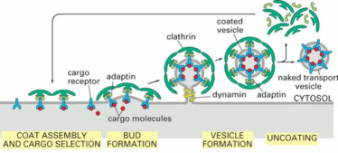
(a) (b)

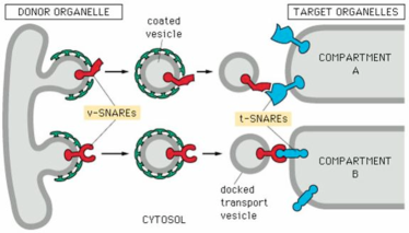
Figure 3: (a) Vesicle formation, (b) Vesicle docking. (Pictures taken from [2])

Let $\mathcal{P}_{p}=\{R_{i}^{e},R_{i}^{c},C_{i},Ad_{i},Cl,Sn_{i}^{e},Sn_{i}^{c},tSn_{i}^{e},tSn_{i}^{c}\}$ and $\mathcal{P}_{ap}=\{R_{i}^{m},Sn_{i}^{m},tSn_{i}^{m}\}$, for $i\in\{0,1\}$. Transmembrane proteins are represented by three sub-units in order to specify the direction they exhibit with respect to membranes into which are embedded. We denote with $R_{i}^{c}(1+2)$, $R_{i}^{m}(1+2)$, $R_{i}^{e}(1+2)$ the three cargo receptor sub-units, respectively for cytosolic, trans-membrane, and extra-cytosolic; SNAREs ($Sn^{*}_{i}$ and $tSn^{*}_{i}$) are defined in a similar way. $C_{i}(1)$ denotes a cargo molecule, $Ad_{i}(1+2)$ adaptin, and $Cl(1)$ clathrin. Proteins are sub-scripted with an index $i\in\{0,1\}$ to distinguish different families of proteins.

We describe the Bio$\beta$ model for membrane traffic giving the set of reaction rules for proteins and introduction of mobility. Protein reactions are defined as follows:

$$\langle C_{i}(1)\ast R_{i}^{e}(1+2^{x}),R_{i}^{c}(1^{y}+\bar{2})\mid R_{i}^{m}(1^{x}+2^{y})\rangle \xrightarrow{\textsf{rec}}\nu z.\langle C_{i}(1^{z})\ast R_{i}^{e}(1^{z}+2^{x})\mathbin{,}R_{i}^{c}(1^{y}+2)\mid R_{i}^{m}(1^{x}+2^{y})\rangle$$

$$\langle R_{i}^{c}(1^{x}+2)\ast Ad_{i}(1+\bar{2})\mid\rangle \xrightarrow{\textsf{adpt}}\nu y.\langle R_{i}^{c}(1^{x}+2^{y})\ast Ad_{i}(1^{y}+2)\mid\rangle$$

$$\langle Ad_{i}(1^{x}+2)\ast Cl(1)\mid\rangle \xrightarrow{\textsf{coat}}\nu y.\langle Ad_{i}(1^{x}+2^{y})\ast Cl(1^{y})\mid\rangle$$

$$\nu y.\langle R_{i}^{c}(1^{x}+2^{y})\ast Ad_{i}(1^{y}+2^{z})\ast Cl(1^{z})\mid\rangle \xrightarrow{\textsf{uncoat}}\langle R_{i}^{c}(1^{x}+2)\ast Ad_{i}(1+2^{z})\ast Cl(1^{z})\mid\rangle$$

$$\langle Sn_{i}^{c}(1^{x}+2)\ast tSn_{i}^{c}(1+2^{z})\mid\rangle \xrightarrow{\textsf{snare}}\nu y.\langle Sn_{i}^{c}(1^{x}+2^{y})\ast tSn_{i}^{c}(1^{y}+2^{z})\mid\rangle$$

Intuitively, (rec) describes the formation of a bond between the cargo molecule and the corresponding cargo receptor, which toggles to visible the hidden site of the receptor cytosolic sub-unit. (adpt) and (coat) allow for the creation of the clathrin coat which leads to the formation of the bud. (uncoat) frees the vesicle from the adaptin-clathrin coat. Finally, (snare) deals with the snare-mediated docking of the naked vesicle, by forming a bond between the v-SNARE and t-SNARE of the same family. Figure 3 gives an informal idea of how protein reactions work.

Introduction rules are defined by the two sets of pinching and fusing configurations: $\mathcal{R}_{\mathsf{p}}$ and $\mathcal{R}_{\mathsf{f}}$.

$$\mathcal{R}_{\mathsf{p}}=\{(P,P^{\prime},S,S^{\prime},Q)\}\quad \text{where}\quad\begin{aligned} P&=C_{i}(1^{x})\ast R_{i}^{e}(1^{x}+2^{y})\ast Sn_{i}^{e}(1^{z})&P^{\prime}&=\diamond\\ S&=R_{i}^{m}(1^{y}+2^{w})\star Sn_{i}^{m}(1^{z}+2^{u})&S^{\prime}&=\mathbf{0}\\ Q&=R_{i}^{c}(1^{w}+2^{a})\ast Ad_{i}(1^{a}+2^{b})\ast Cl(1^{b})\ast Sn_{i}^{c}(1^{u}+2)\end{aligned}$$

The configuration $(P,P^{\prime},S,S^{\prime},Q)$ allows the vesicle to detach when the adaptin-clathrin coat completely cover the forming bud. For sake of simplicity we consider coats of size one, i.e. with only one adaptin-clathrin complex (generalization to coat of size $n$ is straightforward).

$$\mathcal{R}_{\mathsf{f}}=\{(P,S,R,T,Q)\}\quad \text{where}\quad\begin{aligned} P&=C_{i}(1^{x})\ast R_{i}^{e}(1^{x}+2^{y})\ast Sn_{i}^{e}(1^{a})&T&=tSn_{i}^{m}(1^{d}+2^{e})\\ S&=R_{i}^{m}(1^{y}+2^{z})\star Sn_{i}^{m}(1^{a}+2^{b})&Q&=tSn_{i}^{e}(1^{e})\\ R&=R_{i}^{c}(1^{z}+2)\ast Sn_{i}^{c}(1^{b}+2^{c})\ast tSn_{i}^{c}(1^{c}+2^{d})\end{aligned}$$

The configuration $(P,S,R,T,Q)$ describe the situation when the vesicle is docked to the target membrane, hence the fusion can take place.

One possible initial configuration can be defined as follows:

$$Main =DOrg\ast Targ_{0}\ast Targ_{1}$$

$$DOrg =Cl(1)\ast Cl(1)\ast Ad_{0}(1+\bar{2})\ast Ad_{1}(1+\bar{2})\ast R_{0}^{c}(1^{y_{0}}+\bar{2})\ast R_{1}^{c}(1^{y_{1}}+\bar{2})\ast Sn_{0}^{c}(1^{b_{0}}+2)\ast Sn_{1}^{c}(1^{b_{1}}+2)\ast{}$$

$$\phantom{{}={}}\Lbag R_{0}^{m}(1^{x_{0}}+2^{y_{0}})\star R_{1}^{m}(1^{x_{0}}+2^{y_{1}})\star Sn_{0}^{m}(1^{a_{0}}+2^{b_{0}})\star Sn_{1}^{m}(1^{a_{1}}+2^{b_{1}})$$

$$\phantom{{}={}R_{0}^{m}(1^{x_{0}}+2^{y_{0}})\star R_{1}^{m}(1^{x_{0}}+2^{y_{1}})}\,\lbag R_{0}^{e}(1+2^{x_{0}})\ast R_{1}^{e}(1+2^{x_{1}})\ast Sn_{0}^{e}(1^{a_{0}})\ast Sn_{1}^{e}(1^{a_{1}})\ast C_{0}(1)\ast C_{1}(1)\rbag\Rbag$$

$$Targ_{0} =tSn_{0}^{c}(1+2^{d_{0}})\ast\Lbag tSn_{0}^{m}(1^{d_{0}}+2^{e_{0}})\lbag tSn_{0}^{e}(1^{e_{0}})\rbag\Rbag$$

$$Targ_{1} =tSn_{1}^{c}(1+2^{d_{0}})\ast\Lbag tSn_{1}^{m}(1^{d_{1}}+2^{e_{1}})\lbag tSn_{1}^{e}(1^{e_{1}})\rbag\Rbag$$

In this case we have a single donor organelle which is able to pinch out two vesicles (using two different type of SNAREs). Such vesicle can approach the corresponding docking membrane. In Figure 3(b) is depicted a possible run of computation.

4 Comparing with $\kappa$-calculus

In this section we give a formal connection between Bio$\beta$ and Danos and Laneve’s $\kappa$-calculus [8]. This calculus has been taken as the formal model protein interactions in the definition of biobigraphs, the bigraphical model underlying the Bio$\beta$ Framework.

The syntax of $\kappa$-solutions is the following:

$$S,T::=\mathbf{0}\mid A(\rho)\mid S\mathbin{,}T\mid(x)(S)$$

A $\kappa$-solution can be either the empty solution $\mathbf{0}$, or a protein $A(\rho)$, or a group of solutions $S\mathbin{,}T$, or a solution prefixed by name restriction $(x)(S)$ with $x\in\mathcal{N}$.

As usual in process calculi, a structural equivalence ($\equiv$) over processes is introduced, which is the least structural containing $\alpha$-equivalence and satisfying the abelian monoid on composition and the scope extension and extrusion laws. Moreover we define the sets of free edge names $fn(\rho)$ and $fn(S)$, on interfaces and solutions, defined in the common way, where the new name constructor $(x)(S)$ is the only name binder. We say a $\kappa$-solution $S$ is closed iff $fn(S)=\emptyset$.

Connectedness of a $\kappa$-solutions is particular a simper case of the one seen before.

Definition 4.1 (Connectedness and complexes).

Connected $\kappa$-solutions are defined inductively as:

$$\frac{}{A(\rho)}\qquad\displaystyle\frac{S}{(x)(S)}\qquad\displaystyle\frac{S\quad T\quad fn(S)\cap fn(T)\neq\emptyset}{S\mathbin{,}T}\qquad\displaystyle\frac{S\quad S\equiv T}{T}$$

A $\kappa$-solution $S$ is a complex if it is closed, graph-like, and connected.

The semantic of $\kappa$-calculus is defined by means of a transition system built up by a user-defined set of monotone and anti-monotone rules $\mathcal{R}_{\kappa}$.

Definition 4.2 (Growing relation).

A growing relation $\rhd$ over $\kappa$-solutions is defined inductively as:

$$\frac{\displaystyle}{\displaystyle\tilde{x}\vdash\mathbf{0}\rhd\mathbf{0}}\qquad\frac{\displaystyle\tilde{x}\vdash S\rhd T\quad\tilde{x}\vdash\rho\rhd\sigma}{\displaystyle\tilde{x}\vdash S\mathbin{,}A(\rho)\rhd T\mathbin{,}A(\sigma)}\qquad\frac{\displaystyle\tilde{x}\vdash S\rhd T\quad fn(\sigma)\subseteq\tilde{x}}{\displaystyle\tilde{x}\vdash S\rhd T\mathbin{,}A(\sigma)}$$

Again, monotonicity is a simplification of the one shown for Bio$\beta$.

Definition 4.3 (Monotone reactions).

Let $L,R$ be two $\kappa$-solutions. $L\rightarrow(\tilde{x})R$ is a monotone reaction if $\tilde{x}\vdash L\rhd R$, where $L,(\tilde{x})R$ graph-like and $R$ connected. $(\tilde{x})L\rightarrow R$ is antimonotone if $R\rightarrow(\tilde{x})L$ is monotone.

Finally, we are able to characterize a protein transition system:

Definition 4.4 (Protein transition systems).

Given a set $\mathcal{R}_{\kappa}$ of monotone and antimonotone reactions, we define a protein transition system (PTS) as a pair $\langle\mathcal{S},\leadsto\rangle$, such that $\mathcal{S}$ is a set of $\kappa$-solutions, and $\leadsto$ is the least binary relation over $\mathcal{S}$ such that $\mathcal{R}_{\kappa}\subseteq{\leadsto}$, closed w.r.t. $\equiv$, composition and name restriction.

Now we are able to establish formally a connection between the Bio$\beta$ framework and the $\kappa$-calculus, that is all protein reactions that can be take place in our systems are justifiably by means of protein reactions in a $\kappa$-solution. In order to do this, first we show a way to translate Bio$\beta$ systems and reactions into $\kappa$ solutions and reactions ($\llbracket-\rrbracket$). $\llbracket-\rrbracket$ is defined as follows:

$$\begin{aligned} \llbracket\diamond\rrbracket&=\mathbf{0}\\ \llbracket\mathbf{0}\rrbracket&=\mathbf{0}\\ \llbracket\mathsf{p}_{n}\fatsemi P\rrbracket&=\llbracket P\rrbracket\end{aligned}\qquad\begin{aligned} \llbracket A_{p}(\rho)\rrbracket&=A_{p}(\rho)\\ \llbracket A_{ap}(\rho)\rrbracket&=A_{ap}(\rho)\\ \llbracket\mathsf{f}_{n}\fatsemi P\rrbracket&=\llbracket P\rrbracket\end{aligned}\qquad\begin{aligned} \llbracket P\ast Q\rrbracket&=\llbracket P\rrbracket\mathbin{,}\llbracket Q\rrbracket\\ \llbracket S\star T\rrbracket&=\llbracket S\rrbracket\mathbin{,}\llbracket T\rrbracket\\ \llbracket\mathsf{p}^{\perp}_{n}\fatsemi S\rrbracket&=\llbracket S\rrbracket\end{aligned}\qquad\begin{aligned} \llbracket\Lbag S\lbag P\rbag\Rbag\rrbracket&=\llbracket S\rrbracket\mathbin{,}\llbracket P\rrbracket\\ \llbracket\nu n.P\rrbracket&=(n)(\llbracket P\rrbracket)\\ \llbracket\mathsf{f}^{\perp}_{n}\rrbracket&=\mathbf{0}\end{aligned}$$

Such encoding induces a type system over the $\kappa$-solution for checking if the solutions are graph-like. It can be given as follows:

$$(\textsf{zero})\ \frac{}{\emptyset;\emptyset\vdash\mathbf{0}}\qquad\qquad\qquad\frac{A\in\mathcal{P}\quad\forall x\in fn(\rho).|\rho,x|<2}{\{x\in fn(\rho)\mid|\rho,x|=1\};\{x\in fn(\rho)\mid|\rho,x|=2\}\vdash A(\rho)}\ (\textsf{prot})$$

$$(\textsf{res})\ \frac{\Gamma_{1};\Gamma_{2}\vdash S\quad x\notin\Gamma_{1}}{\Gamma_{1};\Gamma_{2}\setminus\{x\}\vdash(x)S}\qquad\qquad\frac{\Gamma_{1},\Gamma;\Gamma_{2}\vdash S\quad\Delta_{1},\Gamma;\Delta_{2}\vdash T\quad(\Gamma_{1}\cup\Gamma_{2})\cap(\Delta_{1}\cup\Delta_{2})=\emptyset}{\Gamma_{1},\Delta_{1};\Gamma_{2},\Delta_{2},\Gamma\vdash S\mathbin{,}T}\ (\textsf{par})$$

The following properties stating a statical relation between Bio$\beta$ and $\kappa$ hold.

Proposition 4.1 (Syntax).

1. For $S$ a $\kappa$-solution, if $\Gamma_{1};\Gamma_{2}\vdash S$ and $\Delta_{1};\Delta_{2}\vdash S$ then $\Gamma_{1}{=}\Delta_{1}$ and $\Gamma_{2}{=}\Delta_{2}$.

2. For $S$ a $\kappa$-solution, $S$ is graph-like iff $\Gamma_{1};\Gamma_{2}\vdash S$ for some $\Gamma_{1},\Gamma_{2}$.

3. For $S,T$ two $\kappa$-solutions, if $S\equiv T$, then $\Gamma_{1};\Gamma_{2}\vdash S$ iff $\Gamma_{1};\Gamma_{2}\vdash T$.

4. For $P$ a Bio$\beta$ system, if $\Gamma_{1};\Gamma_{2}\vdash P:\tau$, then $\Gamma_{1};\Gamma_{2}\vdash\llbracket P\rrbracket$.

Finally, we can state and prove the following semantics/dynamic relation between Bio$\beta$ and $\kappa$:

Proposition 4.2 (Semantics).

1. For $S,T$ two $\kappa$-solutions, if $\Gamma_{1};\Gamma_{2}\vdash S$ and $S\leadsto T$, then $\Gamma_{1};\Gamma_{2}\vdash T$.

2. For a wide monotone protein reaction $(\langle\vec{P},\vec{S}\rangle,\nu\vec{x}.\langle\vec{P}^{\prime},\vec{S}^{\prime}\rangle)\in\mathcal{R}$, and for every $C[\vec{X},\vec{Y}]$ such that $C[\vec{P},\vec{S}]$ is well-formed, then $\llbracket C[\vec{P},\vec{S}]\rrbracket\leadsto\llbracket\nu\vec{x}.C[\vec{P}^{\prime},\vec{S}^{\prime}]\rrbracket$.

3. For a wide anti-monotone protein reaction $(\nu\vec{x}.\langle\vec{P},\vec{S}\rangle,\langle\vec{P}^{\prime},\vec{S}^{\prime}\rangle)\in\mathcal{R}$, for every $C[\vec{X},\vec{Y}]$ such that $\nu\vec{x}.C[\vec{P},\vec{S}]$ is well-formed, then $\llbracket\nu\vec{x}.C[\vec{P},\vec{S}]\rrbracket\leadsto\llbracket C[\vec{P}^{\prime},\vec{S}^{\prime}]\rrbracket$.

Intuitively, this proposition states that every protein transition performed in the Bio$\beta$ framework is justified by a corresponding transition in the $\kappa$-calculus. The converse does not hold, due to the compartment confinements: not all reactions of the translation of a Bio$\beta$ system which are possible in $\kappa$-calculus, correspond effectively to some wide (anti)monotone protein reactions in the Bio$\beta$ framework.

5 Related works

In literature several other calculi, covering both protein reactions and membrane interactions, have been proposed. Two particularly interesting cases are the bio$\kappa$-calculus [9] and the $\mathcal{C}$-calculus [7]. In this section we compare our framework with these calculi analyzing analogies and differences of the approaches.

bio$\kappa$-calculus

can be seen as a version of the $\kappa$-calculus extended with compartments. Compared to Bio$\beta$, the most remarkable similarities are at the syntactic level. Both calculi have a compartment constructor which embeds proteins into membranes, and similar well-formedness conditions to restrict to only biological relevant processes. Both calculi are sound at protein level in the sense of the $\kappa$-calculus. In both cases preservation of well-formedness during reactions is proved, although bio$\kappa$-calculus does not have a formal type system as Bio$\beta$.

Several differences emerge at the semantic level, though. An important design choice distingushing bio$\kappa$ and Bio$\beta$ concerns how the behaviour of a compartment is specified. In bio$\kappa$, the mobility capabilites of a compartment are indicated by its name, which appears explicitly in the rearrangement rules which can be applied. The result of a membrane interaction is one or more new membranes whose names have to be specified in the rearrangement rule. This means that the rule defines also the future (mobility) behaviour of the resulting systems; hence it is up to the modeller to specify correctly the evolutions of names of membranes.

On the other hand, in Bio$\beta$ compartments have no names: membranes are just containers and their behaviour is completely determined by the interactions of proteins floating in the aqueous solutions and lipid bi-layers. Therefore, a modeller has only to provide protein-level rules and define the configurations which trigger a mobility reaction. One does not have to declare how a membrane will evolve (i.e., “which is the next name” in bio$\kappa$), because the behaviour is defined by the rules of the framework.

Due to these radically different design choices, a formal comparison at the semantic level between bio$\kappa$-calculus and Bio$\beta$ is not easy. Moreover, the bio$\kappa$ semantics is given by means of an LTS, instead Bio$\beta$ has a reaction (reduction) relation. A possible future work is to derive an LTS with associated congruential bisimilarity, taking advantage of the theory of bigraphs.

$\mathcal{C}$-calculus

Both $\mathcal{C}$-calculus and Bio$\beta$ frameworks are founded on bigraphical reactive systems, which does not only confer a formal graphical representation but provides also a powerful categorical theory for automatically constructing labelled transition systems (LTSs) whose bisimilarities are always congruences. Even though $\mathcal{C}$-calculus and Bio$\beta$ share common sources of inspiration, they differs in many aspects, one of which is the way compartment reconfiguration are performed.

$\mathcal{C}$-calculus adopts meta-biological “gates” to represent a semi-fused intermediate state in membrane fusion or fission. Gates act like channels, allowing protein diffusion between compartments, and it does not allow for phagocytosis. Moreover, one of the aim of Bio$\beta$ framework is to characterize higher-level membrane interactions with lower-level protein reactions, and to be adequate with respect to the $\kappa$-calculus; a formal connection between $\mathcal{C}$-calculus and $\kappa$-calculus has not been investigated yet. Finally, in the $\mathcal{C}$-calculus, mobility and protein reactions are more intertwined, since membrane interactions are in many steps: introduction of gates, some protein diffusions, and deletion of gates. This mechanism does not provide an explicit, logical separation between compartment reconfiguration and protein reactions. On the other hand, the Bio$\beta$ framework aims to an explicit distinction between protein reactions and mobility actions, as implemented by means of introduction rules, which freeze the subsystems involved in the rearrangement until the structural reconfiguration is actually performed.

6 Conclusion

In this paper we have presented the Bio$\beta$ Framework, a language for both (lower-level) protein and (higher-level) membrane interactions of living cells. A typed language has been given for describing only biologically meaningful compartments and proteins.

In the Bio$\beta$ framework membrane reconfigurations are logically different from protein reactions, but the connection between the two aspects is formally specified. In fact, membrane activities can be motivated by a formal biological justification in terms of protein interactions. Notably, protein interactions are adequate with respect to the $\kappa$-calculus.

As an example application of this framework, we have modelled the mechanism of membrane traffic, which consists in formation, transportation and docking of vesicles.

Related and future work. Due to lack of space, we have omitted a formal connection between the proposed framework and its inspiring bigraphical model. Another interesting aspect to investigate is the bisimilarity definable via the IPO construction on bigraphs [10], which is always a congruence. This can be useful e.g. in synthetic biology, for instance, to verify if a synthetic protein (or even a subsystem to be implanted) behaves as the natural one. We plan to describe such results in a forthcoming work.

Another interesting investigation is to give a formal comparison of Bio$\beta$ with the other two framework present in literature, such as bio$\kappa$ and $\mathcal{C}$-calculus. In particular, it could be useful to understand the differences of $\mathcal{C}$-calculus rule generators and our introduction rules, even because they are both inspired by bigraphical wide reactions.

As a next step, a stochastic version of the Bio$\beta$ framework should be analyzed for simulation purposes. One way could be trying to adapt the extended Gillespie simulation algorithm [11], that works for calculi with multi-compartments.

References

- [1] Alan Aderem and David M. Underhill. Mechanisms of phagocytosis in macrophages. Annual Review of Immunology, 17(1):593–623, 1999. PMID: 10358769.
- [2] Bruce Alberts, Dennis Bray, Karen Hopkin, Alexander Johnson, Julian Lewis, Martin Raff, Keith Roberts, and Peter Walter. Essential Cell Biology, 2nd edition. Garland, 2003.
- [3] Giorgio Bacci, Davide Grohmann, and Marino Miculan. Bigraphical models for protein and membrane interactions. In Gabriel Ciobanu, editor, Proc. MeCBIC’09, EPTCS, 2009.
- [4] Luca Cardelli. Brane calculi. In Vincent Danos and Vincent Schächter, editors, Proc. CMSB, volume 3082 of Lecture Notes in Computer Science, pages 257–278. Springer, 2004.
- [5] Luca Cardelli. Abstract machines of systems biology. T. Comp. Sys. Biology, 3737:145–168, 2005.
- [6] Luca Cardelli. Bitonal membrane systems: Interactions of biological membranes. Theoretical Computer Science, 404(1-2):5 – 18, 2008. Membrane Computing and Biologically Inspired Process Calculi.
- [7] Troels Christoffer Damgaard, Vincent Danos, and Jean Krivine. A language for the cell. Technical Report TR-2008-116, IT University of Copenhagen, December 2008.
- [8] Vincent Danos and Cosimo Laneve. Formal molecular biology. Theoretical Computer Science, 325, 2004.
- [9] Cosimo Laneve and Fabien Tarissan. A simple calculus for proteins and cells. Theor. Comput. Sci., 404(1-2):127–141, 2008.
- [10] Robin Milner. Pure bigraphs: Structure and dynamics. Information and Computation, 204(1):60–122, 2006.
- [11] Cristian Versari and Nadia Busi. Stochastic simulation of biological systems with dynamical compartment structure. In Muffy Calder and Stephen Gilmore, editors, Proc. CMSB, volume 4695 of Lecture Notes in Computer Science, pages 80–95. Springer, 2007.