Keck constraints on a varying fine-structure constant: wavelength calibration errors

Abstract

The Keck telescope’s High Resolution Spectrograph (HIRES) has previously provided evidence for a smaller fine-structure constant, $\alpha$, compared to the current laboratory value, in a sample of 143 quasar absorption systems: $\hbox{$\Delta\alpha/\alpha$}=(-0.57\pm 0.11)\times 10^{-5}$. The analysis was based on a variety of metal-ion transitions which, if $\alpha$ varies, experience different relative velocity shifts. This result is yet to be robustly contradicted, or confirmed, by measurements on other telescopes and spectrographs; it remains crucial to do so. It is also important to consider new possible instrumental systematic effects which may explain the Keck/HIRES results. Griest et al. (2009, arXiv:0904.4725v1) recently identified distortions in the echelle order wavelength scales of HIRES with typical amplitudes $\pm$250 ${\rm m\,s}^{-1}$. Here we investigate the effect such distortions may have had on the Keck/HIRES varying $\alpha$ results. Using a simple model of these intra-order distortions, we demonstrate that they cause a random effect on $\Delta\alpha/\alpha$ from absorber to absorber because the systems are at different redshifts, placing the relevant absorption lines at different positions in different echelle orders. The typical magnitude of the effect on $\Delta\alpha/\alpha$ is $\sim$$0.4\times 10^{-5}$ for individual absorbers which, compared to the median error on $\Delta\alpha/\alpha$ in the sample, $\sim$$1.9\times 10^{-5}$, is relatively small. Consequently, the weighted mean value changes by less than $0.05\times 10^{-5}$ if the corrections we calculate are applied. Unsurprisingly, with corrections this small, we do not find direct evidence that applying them is actually warranted. Nevertheless, we urge caution, particularly for analyses aiming to achieve high precision $\Delta\alpha/\alpha$ measurements on individual systems or small samples, that a much more detailed understanding of such intra-order distortions and their dependence on observational parameters is important if they are to be avoided or modelled reliably.

1 Introduction

The Standard Model of particle physics is parametrized by several dimensionless ‘fundamental constants’, such as coupling constants and mass ratios, whose values are not predicted by the Model itself. Instead their values and, indeed, their constancy must be established experimentally. If found to vary in time or space, understanding their dynamics may require a more fundamental theory, perhaps one unifying the four known physical interactions. One such parameter whose constancy can be tested to high precision is the fine-structure constant, $\alpha\equiv e^{2}/\hbar c$, characterising the strength of electromagnetism. Earth-bound laboratory experiments, conducted over several-year time-scales, which use ultra-stable lasers to compare different atomic clocks based on different atoms/ions (e.g. Cs, Hg⁺, Al⁺, Yb⁺, Sr, Dy; e.g. Prestage et al., 1995), have limited the time-derivative of $\alpha$ to $\dot{\alpha}/\alpha=(-1.6\pm 2.3)\times 10^{-17}{\rm\,yr}^{-1}$ (Rosenband et al., 2008)

Figure 1: Transitions used in MM analyses versus their rest-frame wavelength and their sensitivity to variations in $\alpha$. Note the very different signature of a varying $\alpha$ in absorption systems where only the Mg and Fe ii transitions redwards of 2300 Å are detected and fitted, compared with the more complicated signature for systems containing a subset of the bluer transitions. Note that the relative strengths of the different transitions typically observed in quasar absorption systems is not portrayed here.

Important probes of variations over cosmological space- and time-scales are narrow absorption lines imprinted on the spectra of distant, background quasars by gas clouds associated with foreground galaxies (Bahcall et al., 1967). In particular, electronic resonance transitions from the ground states of metallic atoms and ions are useful indicators of $\alpha$ variation for redshifts up to $\sim$4 – when the universe was $\sim$10 % of its current age – where the transitions are easily accessed from ground-based optical telescopes. The many-multiplet (MM) method (Dzuba et al., 1999; Webb et al., 1999) utilises the relative wavelength shifts expected from different transitions from different multiplets of various atom/ions to measure $\alpha$ from quasar absorption spectra. The velocity shift, $\Delta v_{i}$, of transition $i$ due to a small relative variation in $\alpha$, $\Delta\alpha/\alpha\ll 1$, is determined by the $q$-coefficient for that transition,

$$\omega_{z,i}\equiv\omega_{0,i}+q_{i}\left[\left(\alpha_{z}/\alpha_{0}\right)^{2}-1\right]\,~{}{\rm or}$$ (1)

$$\frac{\Delta v_{i}}{c}\approx-2\frac{\Delta\alpha}{\alpha}\frac{q_{i}}{\omega_{0,i}}\,,$$ (2)

where $\omega_{0,i}$ & $\omega_{z,i}$ are the rest-frequencies in the lab and at redshift $z$, $\alpha_{0}$ is the lab value of $\alpha$ and $\alpha_{z}$ is the shifted value measured from an absorber at $z$. The MM method is the comparison of measured velocity shifts from several transitions (with different $q$-coefficients) to compute the best-fit $\Delta\alpha/\alpha$. Figure 1 illustrates the wavelength shifts experienced by the transitions typically utilized in MM analyses.

Some evidence for $\alpha$-variation has emerged over the last decade from quasar spectra observed with HIRES (Vogt et al., 1994) on the Keck I 10-m telescope in Hawaii. The first tentative evidence in Webb et al. (1999) was subsequently strengthened with larger samples of absorbers (Murphy et al. 2001a; Murphy et al. 2003, hereafter M03). MM analysis of 143 absorption spectra, all from the Keck/HIRES instrument, currently indicate a smaller $\alpha$ in the clouds at the fractional level $\hbox{$\Delta\alpha/\alpha$}=(-0.57\pm 0.11)\times 10^{-5}$ over the redshift range $0.2<\hbox{$z_{\rm abs}$}<4.2$ (Murphy et al., 2004, hereafter M04).

Obviously, confirmation of such a potentially fundamental result must be made with many other telescopes and spectrographs. Similar MM studies using the Ultraviolet and Visual Echelle Spectrograph on the ESO Very Large Telescope in Chile are also beginning to yield constraints on $\Delta\alpha/\alpha$, but none yet rule out (or confirm) the Keck/HIRES results (Murphy et al., 2008). At the same time, further searches for subtle systematic errors which, despite extensive searches (e.g. Murphy et al., 2001b), have evaded detection so far, must be considered in detail. Of particular importance are systematic errors in the wavelength calibration of the quasar spectra, which is usually established using exposures of a standard thorium-argon (ThAr) hollow-cathode emission-line lamp taken immediately before and/or after the quasar exposure. After the wavelength–pixel mapping is derived from the ThAr exposure, that solution is simply applied to the quasar exposure. Since the quasar and ThAr light illuminate the spectrograph slit differently and, in general, take slightly different paths through the spectrograph to the CCD, wavelength calibration errors may ensue.

Griest et al. (2009) (hereafter G09) recently observed a quasar absorption system using Keck/HIRES with an iodine gas absorption cell for more direct wavelength calibration, thereby allowing comparison with the ThAr wavelength scale. For varying-$\alpha$ studies, the most important and robust result from G09 is the identification of distortions in the ThAr wavelength scale across each echelle order (hereafter ‘intra-order distortions’). See their figures 4 and 5. These may result from differential and variable vignetting of quasar light compared to ThAr light, where only the former enters HIRES from the telescope, the optical axes of which differ slightly, causing the quasar light path to rotate as the telescope tracks the quasar (Suzuki et al. 2003; G09). G09 also discuss velocity offsets between the ThAr and I₂ wavelength scales. If those results are robust, they are less important for varying $\alpha$ studies because, as equation (2) makes clear, such velocity offsets will not directly influence a $\Delta\alpha/\alpha$ measurement.

This paper aims to assess the impact these intra-order distortions may have had on the Keck/HIRES results for varying $\alpha$. The following section describes the general effect the distortions will have and provides a crude calculation of their expected magnitude. Section 3 details a more refined calculation of the correction to $\Delta\alpha/\alpha$ for each absorber in the Keck/HIRES sample and Section 4 discusses the results. In section 5 we search for direct evidence for the need to apply the corrections and consider the effect of model errors on our calculations. We conclude in Section 6.

2 The effect of intra-order wavelength distortions

The reason intra-order distortions are problematic for varying $\alpha$ analyses is that they will produce velocity shifts between transitions. For an individual absorption system the transitions will, in general, fall at different positions along different echelle orders and will experience different velocity shifts due to the wavelength calibration distortions. The G09 distortions generally cause blueward shifts which increase towards the echelle order edges in either direction from the center. This pattern seems to be generally repeated on each echelle order. However, because the I₂ cell imprints absorption lines on the quasar spectrum only over the wavelength range $\sim$5000–6200 Å, no information about echelle orders outside this range can be obtained. Nevertheless, it is clear that for two absorbers at different redshifts, possibly with different transitions detected and fitted, different spurious shifts in $\Delta\alpha/\alpha$ will be caused by the intra-order distortions. Indeed, in general, the effect on $\Delta\alpha/\alpha$ will be random in sign and magnitude from absorber to absorber.

A simple illustrative estimate of the expected magnitude of the effect on $\Delta\alpha/\alpha$ in a typical Mg/Fe ii absorber can be calculated as follows. Consider two transitions which, depending on the redshift of the absorber, fall at different positions along their echelle order. If we model the intra-order distortions found by G09 as a simple saw-tooth pattern of peak-to-peak amplitude $\Delta v_{\rm amp}=500\,\hbox{${\rm m\,s}^{-1}$}$ then the root-mean-square (RMS) velocity difference between the two transitions, averaged over redshift, will be $\Delta v_{\rm amp}/(2\!\sqrt{2})=177\,\hbox{${\rm m\,s}^{-1}$}$ if the transitions have arbitrary wavelengths. If one transition is from Mg and the other is from Fe ii, with typical rest wavelengths $\sim$2700 Å (i.e. frequencies $\sim$37000 cm^-1), then the typical difference in $q$-coefficients will be $\sim$1250 cm^-1. The resulting effect on $\Delta\alpha/\alpha$ then follows from equation (2): $\left|\hbox{$\Delta\alpha/\alpha$}_{\rm corr}\right|\sim 0.87\times 10^{-5}$. Adding more transitions will reduce this effect approximately as $\sqrt{N}$. Thus, with typically 4–6 transitions observed in a single absorber, the spurious effect the intra-order distortions will have on its value of $\Delta\alpha/\alpha$ will be $\left|\hbox{$\Delta\alpha/\alpha$}_{\rm corr}\right|\sim 0.4\times 10^{-5}$.

Degradation in the accuracy of the wavelength solution near the order edges was already considered a possibility in Webb et al. (1999). To test the possible effect of this Webb et al. artificially increased the 1-$\sigma$ error bar on $\Delta\alpha/\alpha$ for absorption systems with transitions falling near order edges, thereby down-weighting those systems in the calculation of the weighted mean $\Delta\alpha/\alpha$ for the entire sample. The effect was found to be insignificant. However, a more detailed calculation is clearly warranted given the additional information about the particular form of the intra-order wavelength distortions identified by G09; we carry this out in the following section.

3 Calculating the effect on the Keck/HIRES results

In principle, the best way to understand the effect of intra-order distortions on the Keck/HIRES results would be to correct the wavelength scale of each extracted quasar exposure individually and then combine together exposures of the same quasar to again form the 1-dimensional spectrum. The $\chi^{2}$ minimization of the Voigt profile fits to the absorbers could be run again on the new versions of the combined spectra, producing new, corrected values of $\Delta\alpha/\alpha$. This, clearly, would involve enormous effort and the results would still be subject to possible errors in our model of the intra-order distortions (hereafter ‘model errors’). We therefore take a cruder approach, but one which still allows us to check our expectations that (a) the correction to $\Delta\alpha/\alpha$ should be random in sign and magnitude from absorber to absorber and (b) that the typical correction will be of order $\hbox{$\Delta\alpha/\alpha$}_{\rm corr}\approx 0.4\times 10^{-5}$ as calculated above (Section 2).

We first assume an appropriate functional form to counter the intra-order distortions of G09: a velocity shift increasing from zero at the echelle order centre to $+$500 ${\rm m\,s}^{-1}$ (i.e. a redward shift) at the order edges linearly in wavelength space. We consider a more complex model in Section 5 to illustrate the likely size of model errors in our results.

For each absorption system in the Keck/HIRES sample, we must determine where each transition falls with respect to the order edges to estimate the velocity shifts between all the transitions due to the intra-order distortions. This is complicated by the fact that most quasar spectra used in the analysis were formed by combining extracted spectra of many separate exposures. For each absorption system, we derived the order positions for all relevant transitions from the extracted, wavelength calibrated spectrum for each quasar exposure. Thus, for each transition, $i$, an average velocity shift, $\Delta v_{i}$, was determined assuming that all quasar exposures contributing spectra of that transition did so with equal weight. While the signal-to-noise ratio (${\rm SNR}$) did vary between exposures, this is a good approximation for most absorbers.

From the velocity shifts between the transitions in a given absorber, equation (2) can be used to compute the corresponding correction to the value of $\Delta\alpha/\alpha$. That is, $\hbox{$\Delta\alpha/\alpha$}_{\rm corr}$ is the slope (up to a factor of $-2$) of a linear least-squares fit of the values of $\Delta v_{i}/c$ versus $q_{i}/\omega_{0,i}$. We use values for the laboratory frequencies, $\omega_{0}$, and $q$-coefficients from M03 in these calculations. However, two complications arise here. The first is that not all transitions have spectra of the same ${\rm SNR}$. This is easily remedied by weighting the least squares fit with the squares of the ${\rm SNR}$ values measured from the combined spectra in the continuum around each transition.

The second complication is that the shape of the absorption profile of each transition, and the relative strength of its constituent velocity components, also determine its relative contribution to constraining $\Delta\alpha/\alpha$ in a given absorber. For example, in an absorber with many strong, marginally resolved velocity components, a strong transition may appear very saturated. Thus, the centroids of the velocity components are very weakly constrained, if at all. But if several weaker transitions were also fitted, those velocity components will be optically thin and their centroids will be strongly constrained in the weak transitions. Thus, in this example, the strong transition may not contribute much to the final constraint on $\Delta\alpha/\alpha$ in this absorber. Properly taking this into account is as ‘simple’ as re-running the $\chi^{2}$ minimization of the Voigt profile fits to the absorption profiles after correcting the spectrum of each transition $i$ by its corresponding velocity shift, $\Delta v_{i}$. However, we have ignored this complication, thereby allowing a simpler, more illustrative calculation. Nevertheless, we have tested the importance of this simplification by re-running the $\chi^{2}$ minimization on several absorption systems, at both low- and high-$z$, and find it to be fairly unimportant in most cases.

4 Results

Our estimates of the corrections to $\Delta\alpha/\alpha$ for each of the 143 absorbers in the M04 Keck/HIRES sample, calculated using the method described above, are given in Table 1. These corrections should be added to the original values of $\Delta\alpha/\alpha$, which are also given in the table for convenience. The upper panel of Fig. 2 shows the corrections plotted versus the redshifts of the absorbers. Immediately we notice that the sign and magnitude of the corrections vary randomly from absorber to absorber. Indeed, the mean correction, $(-0.05\pm 0.05)\times 10^{-5}$, is consistent with zero, indicating that there is no strong influence on the average value of $\Delta\alpha/\alpha$, as expected. The median magnitude of the corrections is $0.37\times 10^{-5}$, in line with expectations from the very crude estimate made in Section 2. And while the assumptions required to perform the calculation for each absorber, detailed in the last section, are not unimportant, they should not significantly affect these two main conclusions.

Table 1: Values of $\Delta\alpha/\alpha$ and corrections for possible intra-order distortions of the wavelength scale. The first three columns specify the B1950 quasar name, the emission and absorption redshifts. The fourth column provides the transitions used to determine $\Delta\alpha/\alpha$ in each absorber; each letter represents a transition and the key is provided in table 2 of M03. The fifth column is the raw value of $\Delta\alpha/\alpha$ together with the formal 1-$\sigma$ statistical error. The systematic error term, $\delta(\hbox{$\Delta\alpha/\alpha$})_{\rm sys}$, is non-zero only for “high-contrast” absorbers; see text for explanation. The seventh and eighth columns provide our estimate of the correction, $\hbox{$\Delta\alpha/\alpha$}_{\rm corr}$, for intra-order distortions, to be added to $\Delta\alpha/\alpha$, and the systematic error term, $\delta(\hbox{$\Delta\alpha/\alpha$})^{\rm corr}_{\rm sys}$, which was calculated in the same way as $\delta(\hbox{$\Delta\alpha/\alpha$})_{\rm sys}$ but using the corrected values of $\Delta\alpha/\alpha$. The final column specifies the observational sub-samples employed: A = “Previous low-$z$ sample” from M03; B1 = “Previous high-$z$ sample” from M03; B2 = The 15 absorbers added in M04; C = “New sample” from M03. Only a excerpt of the table is provided here; the complete table is available from the authors or http://astronomy.swin.edu.au/$\sim$mmurphy/pub.html .

B1950 name	$z_{\rm em}$	$z_{\rm abs}$	Transitions	$\Delta\alpha/\alpha$	$\delta(\hbox{$\Delta\alpha/\alpha$})_{\rm sys}$	$\hbox{$\Delta\alpha/\alpha$}_{\rm corr}$	$\delta(\hbox{$\Delta\alpha/\alpha$})^{\rm corr}_{\rm sys}$	Sample
				[$10^{-5}$]	[$10^{-5}$]	[$10^{-5}$]	[$10^{-5}$]
1634$+$7037	1.34	0.99010	bcnpqr	$\phantom{-}1.156\pm 2.399$	0.000	0.498	0.000	A
0019$-$1522	4.53	3.4388	ghl	$\phantom{-}0.937\pm 3.912$	0.000	1.414	0.000	B1
0100$+$1300	2.68	2.3095	efgjklmvw	$-3.949\pm 1.370$	1.754	0.063	1.707	B1

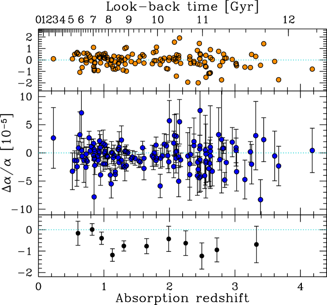
Figure 2: Corrections to $\Delta\alpha/\alpha$ and corrected values of $\Delta\alpha/\alpha$ versus absorption redshift and cosmological look-back time ($H_{0}=71\,\hbox{${\rm km\,s}^{-1}$}\,{\rm Mpc}^{-1}$, $\Omega_{{\rm m,}0}=0.27$, $\Omega_{\Lambda,0}=0.73$). Top: Estimated corrections to $\Delta\alpha/\alpha$ due to intra-order distortions. Note that their sign and magnitude vary randomly from absorber to absorber. The median magnitude of the corrections is $0.37\times 10^{-5}$. Middle: The corrected values of $\Delta\alpha/\alpha$ with their error bars representing the quadrature sum of the 1-$\sigma$ statistical and systematic errors. Bottom: Weighted mean values of $\Delta\alpha/\alpha$, with 1-$\sigma$ errors, in bins containing 13 absorbers each.

It is important to emphasise that the sub-samples of absorbers below and above $\hbox{$z_{\rm abs}$}=1.8$ are qualitatively different. All the absorbers at $\hbox{$z_{\rm abs}$}<1.8$ (‘low-$z$’) depend only on Mg and Fe ii transitions, whereas those at $\hbox{$z_{\rm abs}$}>1.8$ (‘high-$z$’) tend not to include Mg and generally contain the wider variety of transitions, with a mixture of $q$-coefficients, bluewards of $\lambda_{\rm rest}=2300$ Å in Fig. 1. As illustrated in Fig. 1, the signature of a varying $\alpha$ for Mg/Fe ii absorbers is therefore very simple, while that for the higher-$z$ systems is more complicated, strongly depending on which transitions are detected and fitted. In this sense, absorbers with only Mg/Fe ii transitions fitted are more susceptible to simple instrumental systematic errors which cause long-range, low-order distortions of the wavelength scale and also astrophysical effects which might shift velocity components of Fe ii relative to those of Mg. However, for the low-$z$ Mg/Fe ii absorbers in the Keck/HIRES sample, the scatter around the weighted mean $\Delta\alpha/\alpha$ was consistent with the individual error bars in M03 and M04. This remains true even after the corrections for intra-order distortions are applied: $\chi^{2}=76.03$ around the weighted mean $\Delta\alpha/\alpha$ for the 77 low-$z$ absorbers.

The same cannot be said of the high-$z$ absorbers: in M03 and M04 we identified a sub-sample of high-$z$ absorbers for which the scatter in $\Delta\alpha/\alpha$ exceeded expectations based on the individual errors. In these 27 absorbers both very strong and very weak transitions were fitted simultaneously – i.e. they are “high-contrast” absorbers – making the multi-component Voigt profile fitting process more difficult and error-prone. These systems could be ‘under-fitted’ – too few velocity components used to model each absorber – and this may lead to systematic errors in individual absorbers which are random in sign and magnitude. We demonstrated the effect of under-fitting with simulated spectra in Murphy et al. (2008). Just as in M03 and M04, the average systematic error in the sample of 27 high-contrast absorbers is that which, when added in quadrature to the individual statistical errors, reduces $\chi^{2}$ per degree of freedom, $\chi^{2}_{\nu}$, to unity around the weighted mean $\Delta\alpha/\alpha$ for those absorbers. The fact that we find a very similar systematic error term using the corrected values of $\Delta\alpha/\alpha$, $1.71\times 10^{-5}$, as found from the uncorrected values, $1.75\times 10^{-5}$, indicates that the extra scatter in $\Delta\alpha/\alpha$ for these absorbers does not arise from the intra-order distortions; our postulate that it arises from the mixture of strong and weak transitions fitted, and the resulting under-fitting, remains. These systematic error components are shown for the high-contrast absorbers in Table 1.

The middle panel of Fig. 2 shows the corrected values of $\Delta\alpha/\alpha$ with their 1-$\sigma$ statistical errors and systematic error components added in quadrature. The lower panel shows a binned version of these results, where the weighted mean $\Delta\alpha/\alpha$ of the 13 absorbers in each bin is shown with its 1-$\sigma$ error. As with the uncorrected results in see M04, $\Delta\alpha/\alpha$ is consistently smaller $\alpha$ in the absorption systems compared to the current laboratory value. Table 2 quantifies this: the weighted mean $\Delta\alpha/\alpha$ for the full sample, $\hbox{$\Delta\alpha/\alpha$}=(-0.61\pm 0.11)\times 10^{-5}$, differs only slightly from the uncorrected value from M04, $(-0.57\pm 0.11)\times 10^{-5}$, as expected.

Table 2: Basic statistics for the entire sample and redshift sub-samples. The second column gives the number of absorbers, $N_{\rm abs}$, in each sample. The statistics before any corrections for intra-order distortions are applied are in columns 3, 4 & 5, while the remaining columns provide the same statistics after the $\Delta\alpha/\alpha$ values are corrected. $\left<\hbox{$\Delta\alpha/\alpha$}\right>_{\rm w}$ is the weighted mean and $\left<\hbox{$\Delta\alpha/\alpha$}\right>$ is the unweighted mean.

		Before correction				After correction
Sample	$N_{\rm abs}$	$\left<\hbox{$\Delta\alpha/\alpha$}\right>_{\rm w}$	$\left<\hbox{$\Delta\alpha/\alpha$}\right>$	Median		$\left<\hbox{$\Delta\alpha/\alpha$}\right>_{\rm w}$	$\left<\hbox{$\Delta\alpha/\alpha$}\right>$	Median
		[$10^{-5}$]	[$10^{-5}$]	[$10^{-5}$]		[$10^{-5}$]	[$10^{-5}$]	[$10^{-5}$]
Fiducial	143	$-0.57\pm 0.11$	$-0.53\pm 0.19$	$-0.42$		$-0.61\pm 0.11$	$-0.58\pm 0.20$	$-0.56$
$\hbox{$z_{\rm abs}$}<1.8$	77	$-0.54\pm 0.12$	$-0.61\pm 0.22$	$-0.39$		$-0.58\pm 0.12$	$-0.60\pm 0.23$	$-0.58$
$\hbox{$z_{\rm abs}$}>1.8$	66	$-0.74\pm 0.27$	$-0.45\pm 0.34$	$-0.43$		$-0.79\pm 0.27$	$-0.57\pm 0.34$	$-0.55$

Table 2 gives the statistics for the low- and high-$z$ sub-samples. It was shown in M03 that the low- and high-$z$ samples respond, on average, in opposite ways to simple, long-range distortions of the wavelength scale. Note that the weighted means for the low- and high-$z$ absorbers are similar and both depart significantly from zero, even after the corrections are applied. This also quantifies the fact that the evidence for a varying $\alpha$ is dominated by the low-$z$ absorbers, with the evidence at high-$z$ being at the $\approx$3-$\sigma$ level both before and after correction. Still, as mentioned above, if long-range wavelength calibration distortions remain in the data, the low- and high-$z$ samples’ weighted mean $\Delta\alpha/\alpha$ values should have opposite sign. This is an important internal consistency check that is only available when one compares low-$z$ Mg/Fe ii with higher-$z$ absorbers constraining a greater diversity of transitions. Of course, we must also recognise that absence of evidence for systematic errors capable of explaining the consistency of the low- and high-$z$ $\Delta\alpha/\alpha$ values is not evidence for their absence.

5 Are the corrections warranted?

We saw in the previous section that correcting the $\Delta\alpha/\alpha$ values for intra-order distortions of the kind found by G09 makes no difference to the overall conclusions, nor for some more detailed aspects of the Keck/HIRES results. So, having calculated reasonable estimates of the corrections, can we find evidence that applying them really is warranted?

For example, if the corrections are important, we should expect the distribution of $\Delta\alpha/\alpha$ values around the mean to significantly narrow after applying the corrections. We should also expect a significant anti-correlation between the values of $\Delta\alpha/\alpha$ and the corrections. We find neither of these effects.

Table 2 provides the mean $\Delta\alpha/\alpha$ and its standard error – i.e. the RMS/$\sqrt{N_{\rm abs}}$ – for the full sample and low- and high-$z$ sub-samples. Only very small changes in the RMS are evident in each case, indicating that the corrections do not remove a significant amount of scatter in the $\Delta\alpha/\alpha$ values. A small Monte Carlo simulation can be used to gauge how much difference in the RMS we should expect if the corrections were important. We generated random absorber data-sets, with the same size, total errors and corrections as the real Keck/HIRES sample. The corrected $\Delta\alpha/\alpha$ values in each realisation were set to $-0.6\times 10^{-5}$ and then randomised, according to the Gaussian errors for individual absorbers. The RMS of this sample, and the same realisation with the corrections removed from the $\Delta\alpha/\alpha$ values, were compared. Differences in RMS values between the corrected and uncorrected realizations of $>0.1$ and $>0.2\times 10^{-5}$ occurred 37 and 4 % of the time by chance alone. Thus, the lack of RMS differences between our real corrected and uncorrected samples cannot be used as evidence that the corrections are not meaningful. But the Monte Carlo simulation does indicate that the corrections are too small, in comparison to the total errors on $\Delta\alpha/\alpha$ in individual absorbers, to make a large difference to the sample overall.

Similarly, the Spearman rank correlation and Kendall’s $\tau$ tests find insignificant anti-correlations between $\Delta\alpha/\alpha$ and the corrections for the full sample or sub-samples. Nor are absorbers with large $\Delta\alpha/\alpha$ errors masking an underlying anti-correlation; using only absorbers with total errors (quadrature sum of statistical and systematic errors) less than $3\times 10^{-5}$, gives similarly insignificant results. However, again a small Monte Carlo simulation confirms that, effectively, this is not unexpected given the small size of the corrections relative to the larger total errors on individual $\Delta\alpha/\alpha$ values.

To summarise, while we do not find evidence that the corrections we calculate need to be applied, it is their relative smallness in general which precludes a clear test for this. In essence, the formal errors in the Keck/HIRES sample still dominate over the potential systematic errors caused by the intra-order distortions identified by G09.

However, an important assumption so far has been the particular form of intra-order distortion we have used; the G09 results have been approximated with a simple saw-tooth pattern in every echelle order. Because the G09 analysis relies on I₂-cell calibration, it can only probe the intra-order distortions over the wavelength range $\sim$5000–6200 Å. Even over that relatively short wavelength range, there is some evidence for a slow decrease in the peak-to-peak amplitude of the saw-tooth pattern in bluer orders. How this extrapolates to longer and shorter wavelengths than 6200 and 5000 Å (respectively) is unknown. Thus, model errors may well exist in our estimates of the corrections to the Keck/HIRES $\Delta\alpha/\alpha$ values above.

To test the importance of this, we can repeat the calculation of the corrections using a somewhat different model of the intra-order distortions: we fix $\Delta v_{\rm amp}$ to 500 ${\rm m\,s}^{-1}$at 5500 Å and increase (decrease) it linearly with slope 0.55 ${\rm m\,s}^{-1}$ Å^-1 above (below) 5500 Å and enforce a maximum (minimum) amplitude of 1000 ${\rm m\,s}^{-1}$ (200 ${\rm m\,s}^{-1}$) at redder (bluer) wavelengths outside the range covered by the I₂ cell calibration. The RMS difference between the old and new corrections is $0.56\times 10^{-5}$ and, with the new corrections, the weighted mean becomes $(-0.62\pm 0.11)\times 10^{-5}$ over the whole sample and $(-0.61\pm 0.12)\times 10^{-5}$ [$(-0.66\pm 0.27)\times 10^{-5}$] at low$-z$ [high-$z$]. Comparison with the values in Table 2 reveals that the model errors in this case are very small. Of course, this model is not very different to our original, simpler one. For example, it may be that the intra-order distortions have a completely different shape, phase and/or amplitude for different quasar observations. This possibility must be explored with future observations.

6 Conclusions

Exploring systematic effects which may explain the Keck/HIRES evidence for a varying $\alpha$ is clearly an important problem. However, various properties of the Keck/HIRES results make the task difficult; the consistency between the average $\Delta\alpha/\alpha$ values in the low-$z$ Mg/Fe ii and the more diverse high-$z$ systems being an important one. We have demonstrated here that if we model the intra-order distortions identified by G09 in a simple way, and extrapolate the model to all echelle orders (not just those within the I₂-cell calibration range) the effect on the overall evidence for varying $\alpha$ is very small. As expected, the distortions affect individual values of $\Delta\alpha/\alpha$ randomly in sign and magnitude, because the differing redshifts place the transitions at varying positions with respect to echelle order edges where the distortions are worst. Indeed, the effect for a typical absorber is to shift $\Delta\alpha/\alpha$ by $0.4\times 10^{-5}$ which, compared to the median error on $\Delta\alpha/\alpha$, $\sim$$1.9\times 10^{-5}$, is too small for us even to find direct evidence of the need to apply the corrections we calculate.

Despite the above conclusions, it is important to emphasise that we do not yet fully understand the origin of the intra-order distortions identified by G09, how they depend on various observational parameters (e.g. telescope pointing direction, temperature, time etc.) and therefore how they may differently affect spectra of different quasars in the Keck/HIRES sample. Indeed, G09 show that separate exposures taken through the I₂ cell seem to have somewhat different intra-order distortion patterns. And while we have made a simple attempt to address this problem of model errors, it is not enough to completely rule out intra-order distortions as an important systematic error for the Keck/HIRES results. If future Keck/HIRES observations allow much smaller statistical errors on $\Delta\alpha/\alpha$ in individual absorbers or small samples, intra-order distortions like those identified by G09 must either be eliminated or carefully modelled.