Financial rogue waves

Abstract

Abstract.  We analytically present the financial rogue waves in the nonlinear option pricing model due to Ivancevic, which is nonlinear wave alternative of the Black-Scholes model. These rogue wave solutions may be used to describe the possible physical mechanisms for rogue wave phenomenon in financial markets and related fields.

Key words: NLS equation; Nonlinear option pricing model; Financial rogue waves

PACS: 05.45.Yv

I Introduction

Rogue waves have generated many marine misfortunes in the oceans RW1 . The New Year’s wave or Draupner wave was regarded as the first rogue wave recorded by scientific measurement in North Sea. Recently, they were paid much attention in order to understand better their physical mechanisms RW1 ; RW2 ; RW3 ; RW4 ; RW5 ; RW6 ; RW7 ; RW8 . Rogue waves are also known as freak waves, monster waves, killer waves, giant waves, or extreme waves. The rogue wave phenomenon remain poorly understood. It was not until 2007 that Solli et al. ORW first observed the optical rogue waves in an optical fibre and found that they could be used to stimulate supercontinuum generation exp0 . The basic solution (rogon) was first presented by Peregrine PS to describe the rogue wave phenomenon, which was known as by Peregrine soliton (or Peregrine breather). Recently, the multi-rogon solutions were also presented by using the deformed Darboux transformation in ABC ; ABC2 . The matter rogue waves were realized by using the numerical simulation BRW and the rogon-like solutions were also found ypla09 . In addition, the atmospheric rogue waves were also presented arw .

To the best of our knowledge, there is no theoretical research for the financial rogue waves (or financial crisis/storms) that have been occurred (e.g. 1997 Asian financial crisis/storm) and are taking place (e.g. the current global financial crisis/storm).

Based on the the geometric Brownian motion (i.e. the stochastic differential equation) $dS=\mu Sdt+\sigma dW(t)$ satisfied by the stock (asset) price $S$ and the It$\hat{\rm o}$ lemma Ito , the celebrated Black-Scholes linear partial differential equation

$$\frac{\partial C}{\partial t}+\frac{1}{2}\sigma^{2}S^{2}\frac{\partial^{2}C}{\partial S^{2}}+rS\frac{\partial C}{\partial S}-rC=0,$$ (1)

was deduced BS ; BS2 , where $C\equiv C(S,t)$ is the values of European call option on the asset price $S$ at time $t$, $\mu$ is the instantaneous mean return, $\sigma$ is the stock volatility, $W$ is a Wiener process, and $r$ is the risk-free interest rate. In 1997, Merton and Scholes received the Nobel Prize in Economy for their method to determine the price of a European call option. But the model can not describe long-observed features of the implied volatility surface.

II Ivancevic option pricing model

Recently, Ivancevic, based on the modern adaptive markets hypothesis due to Lo Lo ; Lo2 and Elliott wave market theory Elliot ; Elliot2 , and quantum neural computation approach Ivan , proposed a novel nonlinear option pricing model (called the Ivancevic option pricing model)

$$i\frac{\partial\psi(S,t)}{\partial t}=-\frac{1}{2}\sigma\frac{\partial^{2}\psi(S,t)}{\partial S^{2}}-\beta\left|\psi(S,t)\right|^{2}\psi(S,t),$$ (2)

in order to satisfy efficient and behavioral markets, and their essential nonlinear complexity, where $\psi=\psi(S,t)$ denotes the option-price wave function, the dispersion frequency coefficient $\sigma$ is the volatility (which can be either a constant or stochastic process itself), the Landau coefficient $\beta=\beta(r,w)$ represents the adaptive market potential. Some periodic wave solutions of Eq. (2) have been obtained Ivan2 .

III Financial rogue waves

Here, based on the approach developed in  ABC ; ABC2 , we show that the Ivancevic option pricing model (2) also possesses the financial multi-rogon (rogue wave) solutions, which may be used to describe the possible formation mechanisms for rogue wave phenomenon in financial markets. Here we give the first two representative financial rogon solutions of the Ivancevic option pricing model (2).

The financial one-rogon solution of Eq. (2) for the option-price wave function $\psi(S,t)$ by means of the complex rational functions of the stock price $S$ and time $t$ in the form

$$\psi_{1}(S,t)=\alpha\sqrt{\frac{\sigma}{2\beta}}\left[1-\frac{4(1+i\sigma\alpha^{2}t)}{1+2\alpha^{2}(S-\sigma kt)^{2}+\sigma^{2}\alpha^{4}t^{2}}\right]\exp\big{\{}i[kS+\sigma/2(\alpha^{2}-k^{2})t]\big{\}},\ \ \sigma\beta>0\ \$$ (3)

which involves four free parameters $\sigma,\,\beta,\,\alpha$ and $k$ to manage the different types of financial rogue wave propagations whose intensity $|\psi_{1}(S,t)|^{2}$ is displayed in Fig. 1 for the chosen volatility $\sigma=0.3$, adaptive market potential $\beta=0.03$, the scaling $\alpha=2$ and the gauge $k=0,-1.5$. Notice that time $t$ in Fig. 1 can be chosen to be negative since the solution is invariant under the translation transformation $t\rightarrow t+t_{0}$.

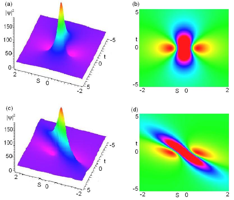
Figure 1: (color online). Rogue wave propagations (left) and contour plots (right) for the intensity $|\psi_{1}|^{2}$ of the one-rogon solution (3) for $\sigma=0.3,\,\beta=0.03,\,\alpha=2$. (a)-(b) $k=0$; (c)-(d) $k=-1.5$.

Moreover, the financial two-rogon solutions of Eq. (2) can be written as

$$\psi_{2}(S,t)=\alpha\sqrt{\frac{\sigma}{2\beta}}\left[1+\frac{P_{2}(S,t)+i\,Q_{2}(S,t)}{R_{2}(S,t)}\right]\exp\big{\{}i[kS+\sigma/2(\alpha^{2}-k^{2})t]\big{\}},\ \ \sigma\beta>0$$ (4)

with these functions $P_{2}(x,t),\ Q_{2}(x,t)$ and $R_{2}(x,t)$ being of polynomial forms of the stock price $S$ and time $t$

$$\begin{array}[]{l}P_{2}(S,t)=\displaystyle\frac{3}{8}-\frac{1}{2}\alpha^{4}(S-\sigma kt)^{4}-\frac{3}{2}\sigma^{2}\alpha^{6}t^{2}(S-\sigma kt)^{2}\vspace{0.08in}\cr\qquad\qquad\displaystyle-\frac{5}{8}\sigma^{4}\alpha^{8}t^{4}-\frac{3}{2}\alpha^{2}(S-\sigma kt)^{2}-\frac{9}{4}\sigma^{2}\alpha^{4}t^{2},\vspace{0.1in}\cr Q_{2}(S,t)=\displaystyle-\frac{1}{2}\sigma\alpha^{2}t\Big{[}\alpha^{4}(S-\sigma kt)^{4}+\sigma^{2}\alpha^{6}t^{2}(S-\sigma kt)^{2}\vspace{0.08in}\cr\qquad\qquad\displaystyle+\frac{1}{4}\sigma^{4}\alpha^{8}t^{4}-3\alpha^{2}(S-\sigma kt)^{2}+\frac{1}{2}\sigma^{2}\alpha^{4}t^{2}-\frac{15}{4}\Big{]},\vspace{0.1in}\cr R_{2}(S,t)=\displaystyle\frac{3}{32}+\frac{1}{12}\alpha^{6}(S-\sigma kt)^{6}+\frac{1}{8}\sigma^{2}\alpha^{8}t^{2}(S-\sigma kt)^{4}\vspace{0.08in}\cr\qquad\qquad\displaystyle+\frac{1}{16}\sigma^{4}\alpha^{10}t^{4}(S-\sigma kt)^{2}+\frac{1}{96}\sigma^{6}\alpha^{12}t^{6}\vspace{0.08in}\cr\qquad\qquad\displaystyle+\frac{1}{8}\alpha^{4}(S-\sigma kt)^{4}-\frac{3}{8}\sigma^{2}\alpha^{6}t^{2}(S-\sigma kt)^{2}\vspace{0.08in}\cr\qquad\qquad\displaystyle+\frac{9}{32}\sigma^{4}\alpha^{8}t^{4}+\frac{9}{16}\alpha^{2}(S-\sigma kt)^{2}+\frac{33}{32}\sigma^{2}\alpha^{4}t^{2},\end{array}$$ (13)

which contains four free parameters $\sigma,\,\beta,\,\alpha$ and $k$ to manage the different types of financial rogue wave propagations whose intensity $|\psi_{2}(S,t)|^{2}$ is depicted in Fig. 2 for the chosen volatility $\sigma=0.3$, adaptive market potential $\beta=0.03$, the scaling $\alpha=0.8$ and the gauge $k=0,-1.5$.

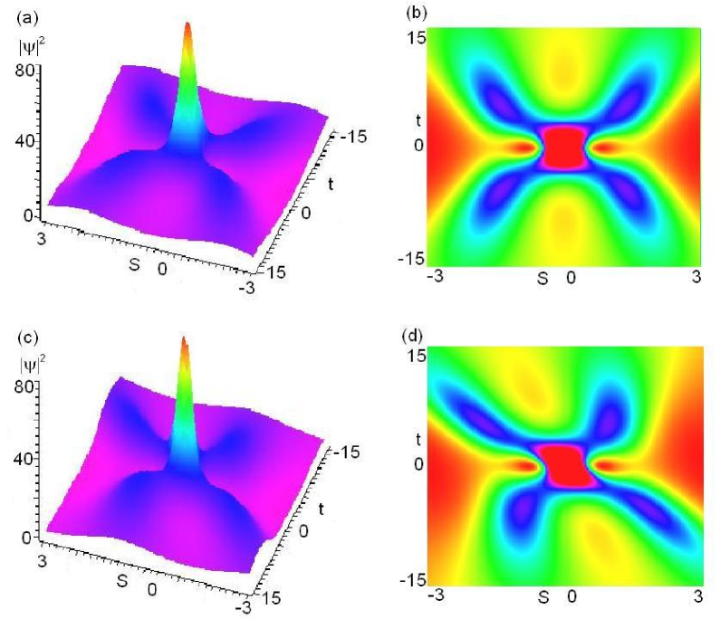
Figure 2: (color online). Rogue wave propagations (left) and contour plots (right) for the intensity $|\psi_{2}|^{2}$ of the one-rogon solution (4) for $\sigma=0.3,\,\beta=0.03,\,\alpha=0.8$. (a)-(b) $k=0$; (c)-(d) $k=-1.5$.

IV Conclusion

In conclusion, we have shown that the nonlinear option pricing model (2) also possesses the analytical financial one- and two-rogon solutions. This may further excite the possibility of relative researches and potential applications for the financial rogue wave phenomenon in the financial markets and related fields.

Acknowledgement The work was supported by the NSFC60821002/F02.

References

- (1)
- (2) G. Lowton, New Sci. 170 (2001) 28.
- (3) L. Draper, Mar. Obs. 35 (1965) 193.
- (4) C. Kharif, E. Pelinovsky, Eur. J. Mech. B (Fluids) 22 (2003) 603.
- (5) P. Müller, Ch. Garrett, A. Osborne, Oceanography 18 (2005) 66.
- (6) A. R. Osborne, Nonlinear Ocean Waves, Academic Press, New York, 2009.
- (7) C. Kharif, E. Pelinovsky, A. Slunyaev, Rogue Waves in the Ocean, Observation, Theories and Modeling, Springer, New York, 2009.
- (8) H. Tamura, T. Waseda, Y. Miyazawa, Geophys. Res. Lett. 36 (2009) L01607.
- (9) K. Dysthe, H. E. Krogstad, P. Müller, Annu. Rev. Fluid Mech. 40 (2008) 287.
- (10) D. R. Solli, C. Ropers, P. Koonath, B. Jalali, Nature 450 (2007) 1054.
- (11) D. R. Solli, C. Ropers, B. Jalali, Phys. Rev. Lett. 101 (2008) 233902.
- (12) D. H. Peregrine, J. Austral. Math. Soc. Ser. B 25 (1983) 16.
- (13) N. Akhmediev, A. Ankiewicz, J. M. Soto-Crespo, Phys. Rev. E 80 (2009) 026601.
- (14) N. Akhmediev, A. Ankiewicz, M. Taki, Phys. Lett. A 373 (2009) 675.
- (15) Yu. V. Bludov, V. V. Konotop, N. Akhmediev, Phys. Rev. A 80 (2009) 033610.
- (16) Z. Y. Yan, Phys. Lett. A 374 (2010) 672.
- (17) L. Stenflo and M. Marklund, arXiv:0911.1654.
- (18) K. It, Mem. Am. Math. Soc. 4 (1951) 1.
- (19) F. Black and M. Scholes, J. Pol. Econ. 81 (1973) 637.
- (20) R. C. Merton, J. Econ. Mana. Sci. 4 (1973) 141.
- (21) A. W. Lo, J. Portf. Manag. 30 (2004) 15.
- (22) A. W. Lo, J. Inves. Consult. 7 (2005) 21.
- (23) A. J. Frost, R. R. Prechter, Elliott Wave Principle: Key to Market Behavior. Wiley, New York, (1978); (10th Edition) Elliott Wave International, (2009)
- (24) P. Steven, Applying Elliott Wave Theory Profitably. Wiley, New York, (2003)
- (25) V. Ivancevic, T. Ivancevic, Quantum Neural Computation, Springer, New York, 2009.
- (26) V. Ivancevic, arXiv:0911.1834.
- (27)