Statistical Regularities of Equity Market Activity

Abstract

Equity activity is an essential topic for financial market studies. To explore its statistical regularities, we comprehensively examine the trading value, a measure of the equity activity, of the $3314$ most-traded stocks in the U.S. equity market and find that (i) the trading values follow a log-normal distribution; (ii) the standard deviation of the growth rate of the trading value obeys a power-law with the initial trading value, and the power-law exponent $\beta=0.14$. Remarkably, both features hold for a wide range of sampling intervals, from $5$ minutes to $20$ trading days. Further, we show that all the $3314$ stocks have long-term correlations, and their Hurst exponents $H$ follow a normal distribution. Furthermore, we find that the Hurst exponent depends on the size of the company. We also show that the relation between the scaling in the growth rate and the long-term correlation is consistent with $\beta=1-H$, similar to that found recently on human interaction activity by Rybski and collaborators.

I Introduction

As a typical complex system, the financial markets attracts many researchers in both economics and physics Kondor99 ; Bouchaud00 ; Mantegna00 ; Johnson03 ; Cizeau97 ; Liu97 ; Liu99 ; Harris86 ; Admati88 ; Plerou01 ; Plerou07 ; Lux00 ; Giardina01 ; Yamasaki05 ; Wang06 ; Wang07 ; Wang09 ; Weber07 ; Ivanov04 ; Eisler06A ; Eisler06B ; Eisler08 . It has been extensively studied over one hundred years, especially in recent few decades, since huge financial databases became available due to the development of electronic trading and data storing. A key issue of these studies is the dynamics of the equity market, including both of the price movement and market activity. Several stylized facts have been found for the equity price movement, such as (i) the distribution of the stock price changes (“return”) has a power-law tail and (ii) the absolute value of price change (“volatility”) is long-term power-law correlated Kondor99 ; Bouchaud00 ; Mantegna00 ; Johnson03 ; Cizeau97 ; Liu97 ; Liu99 ; Harris86 ; Admati88 ; Lux00 ; Giardina01 . These measures have been well studied, for example, a recent approach called return interval analysis has been developed to comprehensively study the temporal structure in the volatility time series Yamasaki05 ; Wang06 ; Wang07 ; Wang09 .

The market activity was also studied by many researchers. Plerou et al. investigated the market activity and found that the number of trades displays long-term power-law correlations and the trading volume follows a Lévy-stable distribution Plerou01 ; Plerou07 . Ivanov et al. studied the inter-trade time and showed multiscaling behavior in its distribution Ivanov04 . Eisler and Kertész analyzed the fluctuation in the trading values and found a certain scaling law Eisler06A ; Eisler06B ; Eisler08 . Moreover, the activity in many other economic and social systems has been studied Gibrat31 ; Zipf32 ; Sutton97 ; Gabaix99 ; Stanley96 ; Rybski09 . For example, recently Rybski et al. studied the dynamics of human interaction activity and showed the connection between the long-term correlations in the activity and scaling in the activity growth Rybski09 . It is important to comprehensively examine the dynamics of the equity activity and test the relation between the correlation and the scaling in the growth rate, which may help to better understand financial markets. In addition, the comparison between the financial markets and other complex systems may shed light on revealing the underlined mechanisms of the complex systems. For this purpose, we study here the equity activity of the U.S. stock market, a representative example of the world financial markets.

The paper is organized as follows: In section II we introduce the database and the variable of trading value which characterizes the equity activity, and demonstrate the intraday pattern for the trading value. In section III we investigate the distribution of the trading values and find that the distribution follows a log-normal function. We also find a power-law relation between the standard deviation of the growth rate of the trading value and the initial trading value, which holds for a wide range of sampling intervals. Section IV deals with the long-term correlations in the time series of the market activity, which is characterized by the Hurst exponent $H$. We show that the Hurst exponents of the stocks follow a normal distribution with $H=0.75\pm 0.09$. In Section V we discuss the relation between the scaling in the growth rate and the long-term correlations, and summarize our findings.

II Data Analyzed

In this paper we analyze the Trades And Quotes (TAQ) database from the New York Stock Exchange (NYSE), which records every transaction for all securities in the U.S. equity market. The period studied is from January 2, 2001 to December 31, 2002 (in total $500$ trading days). However, the number of trading days varies with the stock. To have enough records for analyzing, we only consider the stocks that were traded at least $480$ days. In total we have $3314$ stocks which include $1.42\times 10^{9}$ records. In addition, these stocks have quite different trading frequencies, from $6$ times per day to $6\times 10^{4}$ times per day. To study different stocks on the same footing, we adopt several typical sampling intervals $\Delta T$ in our analysis, including $\Delta T=5$-min, $30$-min, $1$-day, $5$-day ($1$ trading week), and $20$-day (roughly $1$ trading month). Note that $1$ trading day has $390$ minutes in the U.S. market. Thus the range of these sampling intervals is over $3$ order of magnitudes.

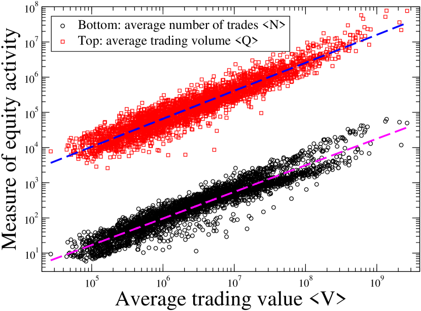
Figure 1: (Color online) Relation between the trading value $V$ and two other measures of the equity activity, number of trades $N$ and trading volume $Q$. Each data point represents the daily average of one stock in the 2001-02 period, and in total $3314$ stocks are plotted. Clearly the three measures are strongly correlated. To further show the tendency, we fit both cases with the power-law, as shown by the dashed lines. The corresponding power-law exponent is $0.76$ for the number of trades and $0.80$ for the trading volume.

The trading activity of an equity can be characterized by several measures, such as the number of trades $N$, trading volume $Q$ (number of shares traded), and trading value $V$ (amount of money traded) in a certain time interval $\Delta T$. To select an activity measure, we first need to test the relation among $V$, $N$, and $Q$. Without loss of generality, we adopt $\Delta T=1$-day. In Fig 1 we plot the average number of trades $\langle N\rangle$ vs. the average trading value $\langle V\rangle$ and the average trading volume $\langle Q\rangle$ vs. the average trading value $\langle V\rangle$. In this paper $\langle...\rangle$ stands for the average over the whole data set. Both cases show straight-line tendencies in the log-log scale, suggesting there are strong dependence between them. The correlation is $0.81$ between $\langle N\rangle$ and $\langle V\rangle$, and $0.86$ between $\langle Q\rangle$ and $\langle V\rangle$. Such strong correlations indicate that the three variables have similar features. In addition, the unit of the trading value (dollar) is the same for all stocks, but the unit of number of trades (times of stock) and trading volume (shares of stock) are all specific to a certain stock, and any two stocks are not the exact same financial asset. Thus we choose the trading value $V$ as the measure of the market activity.

In contrast to daily equity data, the intraday data are known to show specific patterns for measures such as volatility Liu99 ; Harris86 ; Admati88 ; Wang06 , due to different behaviors of traders during a trading day. For example, the market is very active immediately after the opening Admati88 , due to information arriving while the market is closed. A question naturally arises. Is there any intraday pattern in the trading activity? To test this, we investigate the daily trend of the trading value for all the $3314$ stocks. For one stock, the intraday pattern $A(s)$ is defined as

$$A(s)\equiv\frac{\langle V\rangle_{s}}{\langle V\rangle},$$ (1)

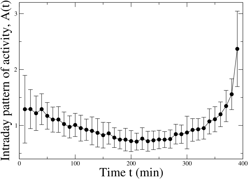
Figure 2: (Color online) Intraday pattern of the trading values. For each stock, we obtain the intraday pattern by computing the average trading value over all trading days for each 10-min time interval, and normalize it with the average activity over all 10-min intervals of this stock. To demonstrate the pattern of all equities in the market, we plot the average and standard deviation (as error bar) over the patterns of all the $3314$ stocks against the time $t$ in a trading day. Clearly we can see that the market activity is not uniform during a trading day. In particular it is relatively intensive in the opening and closing hours, and quiet around noon. Moreover, the differences are significantly large than the error bars, suggesting that this U-shape pattern persists for the entire market. Note that the error bars are larger in the opening and closing hours, which is consistent with the intensive activity in these hours.

Here $\langle V\rangle_{s}$ is the average trading value at a specific moment $s$ of a trading day, and $\langle V\rangle$ is the average trading value over all records. To show the tendency over the whole market, we plot the average of $A(s)$ of all the $3314$ stocks and its standard deviation (as error bar) in Fig. 2. Clearly there is no uniform pattern during a trading day. The pattern has a minimum around noon ($s=200$ min), which is consistent with the intraday pattern found for volatility Liu99 ; Harris86 ; Admati88 ; Wang06 . However, there is a pronounced peak at the closing hours and relative high values at the opening hours, which are opposite to that of volatility where in the opening hours it is higher compared to the closing hours. The volatility is more fluctuating in the opening hours since that lots of news arrive during the market closure and the market needs to rapidly response to them at the opening hours. On the other hand, the investors tend to make decisions after the market takes into account all information and thus more transactions are made in the closing hours. To avoid this daily oscillation, for the intraday data of each stock we divide the trading value with its pattern $A(s)$.

III Scaling in the Trading Value and its Growth Rate

Scaling and universality are two important concepts in statistical physics. A system obeys a scaling law if its components can be characterized by a property having a power-law relation for a broad range of scales (“scale invariance”). A typical behavior for scaling is data collapse: all curves can be “collapsed” onto a single curve, after a certain scale transformation. In many systems, the same scaling function holds, suggesting universal laws. Now we are trying to test whether the market activity has scaling and universality features.

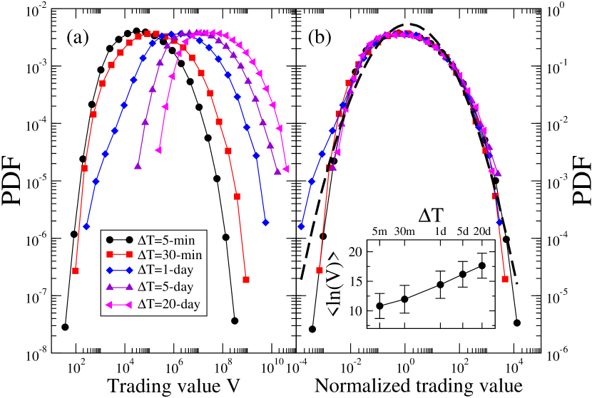
Figure 3: (Color online) Distribution of the trading values. (a) Plot of the probability density functions (PDF) of the trading value for 5 sampling intervals, $\Delta T=5$-min, $30$-min, $1$-day, $5$-day, and $20$-day. Though these curves have different centers and widths, their shapes are similar. To test this similarity, (b) we normalize the trading value for each sampling interval and plot their PDFs. All curves almost collapse into a single one, which can be well-fit by a log-normal distribution (as shown by the dashed line). This result suggests that the trading value follows a log-normal distribution for a sampling interval range over $3$ order of magnitudes. The mean value of $ln(V)$, $\langle ln(V)\rangle$, vs. the sampling interval $\Delta T$ is plotted in the inset of panel (b), where the error bars stand for standard deviations of $ln(V)$, $\sigma(ln(V))$. Note that $\langle ln(V)\rangle$ is logarithmically related to $\Delta T$ and $\sigma(ln(V))$ is almost constant, suggesting that the trading value linearly depends on the sampling interval.

We begin by examining the distribution of the trading values, which can be characterized by a probability density function (PDF) $P$. In Fig. 3(a) we plot the PDFs of $5$ sampling intervals, $\Delta T=5$-min, $30$-min, $1$-day, $5$-day, and $20$-day for all the $3314$ stocks. The distributions shift to the right (large values of $V$) with the increasing of the sampling interval. Interestingly, all the five distributions have a similar shape, which approximately follows a log-normal function,

$$P(V)\sim\exp{(-\frac{(ln(V)-\langle ln(V)\rangle)^{2}}{2\sigma^{2}(ln(V))})}.$$ (2)

In this paper $\sigma(x)\equiv\sqrt{\langle x^{2}\rangle-\langle x\rangle^{2}}$ represents the standard deviation of variable $x$. To further test Eq. (2), we normalize the trading value by replacing $ln(V)$ with $(ln(V)-\langle ln(V)\rangle)/\sigma(ln(V))$ and plot the corresponding PDFs in Fig. 3(b). Remarkably, all curves almost collapse onto a single one. Moreover, these curves can be well-fit by a log-normal function (as shown by the dashed line in Fig. 3(b)). This result supports that the distribution of the trading values follows Eq. (2). We also plot the mean values and standard deviations (as error bars) of $ln(V)$ in the inset of Fig. 3(b). While the mean value of $ln(V)$ increases with $\Delta T$, its standard deviation is almost constant for all the sampling intervals. This behavior further supports the consistency between the trading values over a wide range of sampling intervals, from $5$ minutes to $20$ trading days.

Dynamics of the financial markets is a key issue in econophysics and economics, which is usually characterized by the growth rate. This measure has been well studied for the price, which smoothly evolve with the time for many securities. However, the change in the equity activity might be irregular. There might be few transactions in some periods but many in the other periods. To avoid dramatic fluctuations, we define the growth rate at time $t$, $g(t)$, as the logarithmic change of two consecutive cumulative activities Rybski09 , i.e., for the trading value at time $t-1$, $V(t-1)$, and at time $t$, $V(t)$,

$$g(t)\equiv ln(\frac{V(t-1)+V(t)}{V(t-1)})=ln(1+\frac{V(t)}{V(t-1)}).$$ (3)

We analyze the growth rate of all stocks at all times together, therefore we neglect time $t$ of the growth rate. For simplicity, we denote the initial trading value of the growth rate, $V(t-1)$, as $V_{i}$ in the following. To examine the dynamics of the activity, we study two measures of the growth rate: (i) the conditional mean growth rate $\langle g|V_{i}\rangle$, which quantifies the average growth rate of the trading value given the initial trading value $V_{i}$; (ii) the conditional standard deviation $\sigma(g|V_{i})\equiv\sqrt{\langle g^{2}|V_{i}\rangle-\langle g|V_{i}\rangle^{2}}$, which characterizes the fluctuation of the growth rate conditional on a given initial trading value $V_{i}$.

In Fig. 4(a) we plot the conditional mean value $\langle g|V_{i}\rangle$ vs. initial value $V_{i}$ for the five sampling intervals. Interestingly, all the five curves tend to a constant $ln(2)$ for large $V_{i}$ values (as shown by the dashed line). According to Eq. (3), this behavior suggests that two consecutive trading values tend to be similar for the whole market. In other words, there is certain memory in the time series of trading value. In addition, there is an obviously systematic tendency with the sampling intervals. With the increasing of $\Delta T$, $\langle g|V_{i}\rangle$ decreases and shifts to the right for small $V_{i}$ values, which is due to the limited size of the database. For small $V_{i}$ values, the next trading value is typical the same or larger, thus the corresponding $\langle g|V_{i}\rangle$ value is significantly larger than $ln(2)$. For very large $V_{i}$ values, the next trading values tend to be smaller and thus $\langle g|V_{i}\rangle$ values decrease, as shown in the curves of $\Delta T=5$-min and $30$-min.

Next we plot the conditional standard deviation $\sigma(g|V_{i})$ vs. $V_{i}$ in Fig. 4(b), and find that the curves for the all five sampling intervals collapse onto a single one. Furthermore, these curves follow a power-law function (as guided by the dashed line in Fig. 4(b)),

$$\sigma(g|V_{i})\sim V_{i}^{-\beta},$$ (4)

with the exponent $\beta=0.14\pm 0.02$, which is consistent with the finding on growth rate of other complex systems Stanley96 ; Rybski09 . We must note that this scaling persists for a very broad range of $V_{i}$ values, which covers more than $6$ order of magnitudes. This remarkably behavior indicates a significant universality in the whole equity market.

IV Long-Term Correlations

Many financial time series have memory, where a value in the sequence depends on the previous values. Previous studies have shown that the return does not exhibit any linear correlations extending for more than a few minutes, but the volatility exhibits long-term correlations (see Refs. Mantegna00 and Liu99 for example). Thus, the temporal structure in the equity activity is also of interest. Fig. 4(a) already suggests a certain memory between two consecutive values of $V$. To further test the correlations in the trading value time series, we employ the detrended fluctuation analysis (DFA), a wide-used method to examine the correlations in the time series Peng94 ; Peng95 ; Bunde00 ; Hu01 ; Chen02 ; Kantelhardt02 ; Xu05 . In contrast to the conventional method such as the auto-correlation function, DFA can deals with the non-stationary time series such as financial markets records. After removing trends, DFA computes the root-mean-square fluctuation $F(\ell)$ of a time series within a window of $\ell$ points, and determines the Hurst exponent $H$ from the scaling function,

$$F(\ell)\sim\ell^{H}.$$ (5)

The correlation is characterized by the Hurst exponent $H\in(0,1)$. If $H>0.5$, the records have positive long-term correlations. if $H=0.5$, no correlation (white noise), and if $H<0.5$, it has long-term anti-correlations.

Without loss of generality, we study the long-term correlation in the time series of $\Delta T=5$-min for every stock. As examples, we plot the DFA curves in Fig. 5(a) for the activity of four typical stocks, Natco Group Inc. (NTG), Pharmacopeia Drug Discovery Inc. (PCOP), Molex Inc. (MOLX), and Advanced Micro Devices Inc. (AMD). As seen in the plot, their corresponding Hurst exponent varies in a wide range, from $0.6$ to $0.9$. To investigate the long-term correlations for all the $3314$ stocks, we plot the distribution of the $3314$ $H$ values in Fig. 5(b). Interestingly, this distribution can be well characterized by a normal distribution with a mean value of $0.75$ and standard deviation of $0.09$, as seen by the dashed line in the plot.

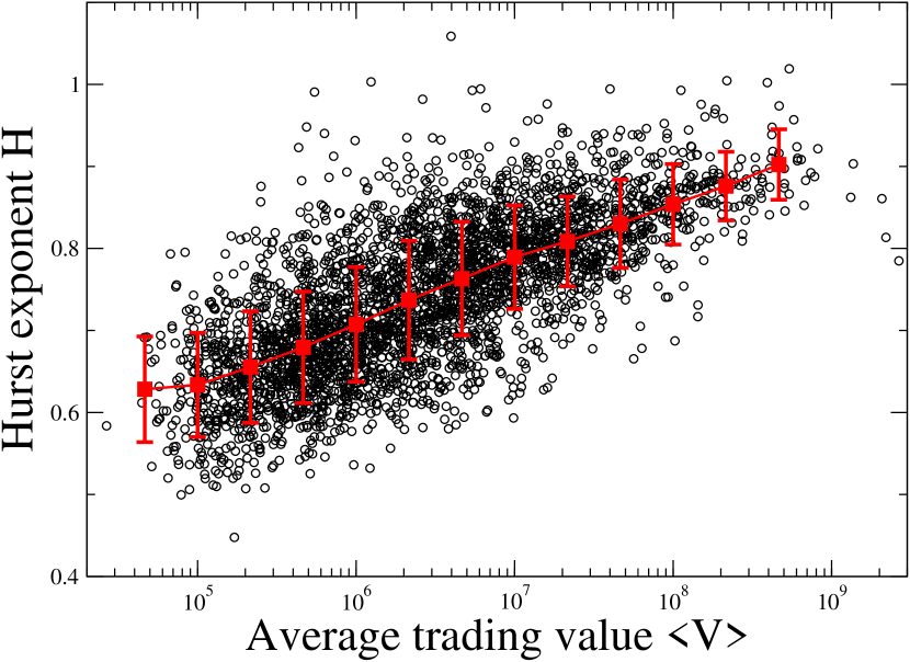
Figure 6: (Color online) Scatter plot of Hurst exponent $H$ vs. average trading value $\langle V\rangle$ for the $3314$ stocks. To better show the tendency, we group the points with similar $\langle V\rangle$ values and plot their mean values (as shown by the filled squares) and standard deviations (as shown by the error bars). It is seen that $H$ depends on the size of $\langle V\rangle$, and their relation approximately follows a logarithmic function, $H\sim 0.033\times ln(\langle V\rangle)$. This finding suggests that the stocks of smaller size are less correlated. It seems that their activities are more influenced by the external factors.

The next question is, why the Hurst exponent $H$ varies with the stock? As we know, there are many factors that relate to the long-term correlations in the financial time series. For example, the long-term correlations in the volatility depends on the size, activity, risk, and return of the stock Wang09 . Thus there might be many factors that affect the long-term correlations in the activity. Here we test the relation between $H$ and the average trading value $\langle V\rangle$ (without loss of generality, we choose the sampling interval of $\Delta T=1$-day for $\langle V\rangle$). The exponent $H$ clearly shows dependence on the value of $\langle V\rangle$, as seen in the scatter plot of Fig. 6. The exponent $H$ of activity tends to increase with $\langle V\rangle$. To better show the tendency, we also plot the average and standard deviation (as the error bar) of $H$ values for every logarithmic bin of $\langle V\rangle$ values, which follows a logarithmic function, $H\sim 0.033\times ln(\langle V\rangle)$. This finding indicates that the long-term persistence is relative weaker for the stocks with smaller $\langle V\rangle$ values. This might be understood since small stocks are easier to be influenced by the external factors and events due to their small size and market depth. Note that the error bars are almost constant for all range of $\langle V\rangle$ values.

V Discussions

As discussed in the Section II, other equity activity measures such as the number of trades and trading volume strongly depends on the trading value. We also explore their features including the scaling of the distributions and the long-term correlations in the activity time series. As expected, they are similar to those obtained for the trading value.

As suggested by Rybski et al. Rybski09 , the exponent $\beta$ and $H$ are related to each other and represent the fluctuations in the time series. Using Eqs. (4) and (5), $\beta$ is determined by the fluctuation of growth and its scaling with the size of the initial activity, and $H$ is generated from the scaling of the fluctuation with the time interval. This leads to the relation between $\beta$ and $H$ Rybski09

$$\beta=1-H.$$ (6)

In our analysis we find $\beta=0.14$ (Fig. 4(b)) and $H$ close to $0.8$ for all the $3314$ stocks (Fig. 5(b)), which roughly satisfies Eq. (6). Fig. 4(b) accumulates all the data points of the $3314$ stocks while the correlations vary with the stock, as demonstrated by Fig. 5(b). To better understand the dynamics of equity activity, the relation between $\beta$ and $H$ should be comprehensively examined, which will be studied in the future.

In summary, we studied the activity of the $3314$ most-traded U.S. stocks. We showed that the equity activity has an intraday pattern. The stock is more traded in the opening hours and significantly more in the closing hours. We found that the distribution of activity follows a log-normal function for all studied sampling intervals. We also found that the conditional standard deviation of growth rate has a power-law dependence on the initial trading value. Moreover, this scaling behavior is persistent for a wide range of sampling intervals, from $5$ minutes to $20$ trading days. Further, we explored the long-term correlations in the time series of the equity activity and found that the correlation exponent $H$ has a normal distribution over the entire market with $H=0.75\pm 0.09$. We also showed that the long-term correlation exponent $H$ depends logarithmically on the size of the activity. In other words, the smaller stock tends to have weaker long-term correlations.

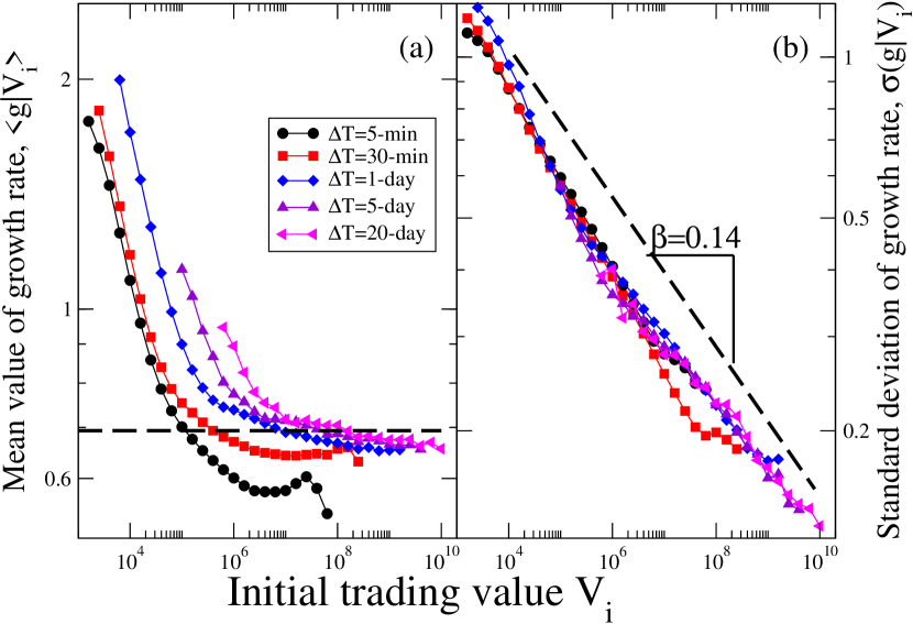
Figure 4: (Color online) Scaling in the growth rate of the trading value. The conditional mean growth rate $\langle g|V_{i}\rangle$ and conditional standard deviation of the growth rate $\sigma(g|V_{i})$ vs. the initial trading value $V_{i}$ are plotted in panel (a) and (b) respectively. Five sampling intervals, $\Delta T=5$-min, $30$-min, $1$-day, $5$-day, and $20$-day, are explored. Remarkably, al curves in panel (a) converge to a constant value, $ln(2)$, as suggested by the dashed line. Thus the two consecutive trading values tend to be the same, which indicates a strong memory in the sequence of the trading value. Note that all curves have large $\langle g|V_{i}\rangle$ values for small $V_{i}$ values, and they shift to the right when the sampling interval is increased. Also note that the curves of $\Delta T=5$-min and $30$-min have small drops for large $V_{i}$ values. Both behaviors are due to the finite size effect in the data. In panel (b), all curves approximately collapse into a single one, which suggests a scaling law for the sampling interval over $3$ order of magnitudes. Moreover, the curves can be well-fit by a power law for the trading value over $6$ order of magnitudes, $\sigma\sim V_{i}^{-\beta}$ with exponent $\beta=0.14\pm 0.02$.

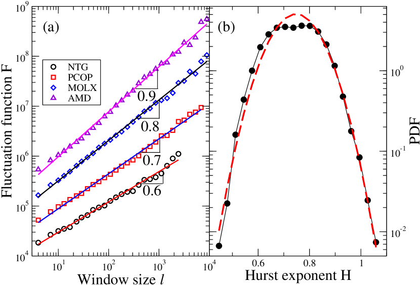
Figure 5: (Color online) Long-term correlation in the time series of the trading value. The time series is for a typical sampling interval, $\Delta T=5$-min. (a) Illustration of the DFA plot, fluctuation function $F$ vs. window size $\ell$. The results of four representative stocks, NTG, PCOP, MOLX, and AMD, are plotted and their Hurst exponents $H$ are labeled in the panel. (b) Distribution of the Hurst exponent $H$ for the 3314 stocks. Note that the distribution can be well-fit by a normal distribution, as shown by the dashed line, with $\langle H\rangle=0.75$ and $\sigma(H)=0.09$.

References

- (1) Econophysics: An Emerging Science, edited by I. Kondor and J. Kertész (Kluwer, Dordrecht, 1999).
- (2) J.-P. Bouchaud and M. Potters, Theory of Financial Risk: From Statistical Physics to Risk Management (Cambridge Univ. Press, Cambridge, England, 2000).
- (3) R. Mantegna and H. E. Stanley, Introduction to Econophysics: Correlations and Complexity in Finance (Cambridge Univ. Press, Cambridge, England, 2000).
- (4) N. F. Johnson, P. Jefferies, and P. M. Hui, Financial Market Complexity (Oxford Univ. Press, New York, 2003).
- (5) P. Cizeau, Y. Liu, M. Meyer, C.-K. Peng, and H. E. Stanley, Physica A 245, 441 (1997).
- (6) Y. Liu, P. Cizeau, M. Meyer, C.-K. Peng, and H. E. Stanley, Physica A 245, 437 (1997).
- (7) T. Lux and M. Marchesi, Int. J. Theor. Appl. Finance 3, 675 (2000).
- (8) I. Giardina and J.-P. Bouchaud, Physica A 299, 28 (2001).
- (9) Y. Liu, P. Gopikrishnan, P. Cizeau, M. Meyer, C.-K. Peng, and H. E. Stanley, Phys. Rev. E 60, 1390 (1999).
- (10) L. Harris, J. Financ. Econ. 16, 99 (1986).
- (11) A. Admati and P. Pfleiderer, Rev. Financ. Stud. 1, 3 (1988).
- (12) F. Wang, K. Yamasaki, S. Havlin, and H. E. Stanley, Phys. Rev. E 73, 026117 (2006).
- (13) K. Yamasaki, L. Muchnik, S. Havlin, A. Bunde, and H. E. Stanley, Proc. Natl. Acad. Sci. U.S.A. 102, 9424 (2005).
- (14) F. Wang, P. Weber, K. Yamasaki, S. Havlin and H. E. Stanley, Eur. Phys. J. B 55, 123 (2007).
- (15) F. Wang, K. Yamasaki, S. Havlin and H. E. Stanley, Phys. Rev. E 79, 016103 (2009).
- (16) P. Weber, F. Wang, I. Vodenska-Chitkushev, S. Havlin, and H. E. Stanley, Phys. Rev. E 76, 016109 (2007).
- (17) V. Plerou, P. Gopikrishnan, X. Gabaix, L. A. N. Amaral, and H. E. Stanley, Quant. Finance 1, 262 (2001).
- (18) V. Plerou and H. E. Stanley, Phys. Rev. E 76, 046109 (2007); E. Ráce, Z. Eisler, and J. Kertész, ibid 79, 068101 (2009); V. Plerou and H. E. Stanley, ibid 79, 068102 (2009).
- (19) P. Ch. Ivanov, A. Yuen, B. Podobnik, and Y. Lee, Phys. Rev. E 69, 056107 (2004).
- (20) Z. Eisler and J. Kertész, Phys. Rev. E 73, 046109 (2006).
- (21) Z. Eisler and J. Kertész, Eur. Phys. J. B 51, 145 (2006).
- (22) Z. Eisler, I. Bartos and J. Kertész, Adv. Phys. 57, 89 (2008).
- (23) R. Gibrat, Les Inégalités Économiques (Libraire du Recueil Sierey, Paris, 1031).
- (24) G. Zipf, Selective Studies and the Principle of Relative Frequency in Language (Harvard Univ Press, Cambridge, MA 1932).
- (25) J. Sutton, J. Econ. Lit. 35, 40 (1997).
- (26) X. Gabaix, Quart. J. Econ. 114, 739 (1999).
- (27) M. H. R. Stanley, L. A. N. Amaral, S. V. Buldyrev, S. Havlin, H. Leschhorn, P. Maass, M. A. Salinger, and H. E. Stanley, Nature 379, 804 (1996).
- (28) D. Rybski, S. V. Buldyrev, S. Havlin, F. Liljeros, and H. A. Makse, Proc. Natl. Acad. Sci. U.S.A. 106, 12640 (2009).
- (29) C.-K. Peng, S. V. Buldyrev, S. Havlin, M. Simons, H. E. Stanley, and A. L. Goldberger, Phys. Rev. E 49, 1685 (1994).
- (30) C.-K. Peng, S. Havlin, H. E. Stanley, and A. L. Goldberger, Chaos 5, 82 (1995).
- (31) A. Bunde, S. Havlin, J. W. Kantelhardt, T. Penzel, J.-H. Peter, and K. Voigt, Phys. Rev. Lett. 85, 3736 (2000).
- (32) K. Hu, P. Ch. Ivanov, Z. Chen, P. Carpena, and H. E. Stanley, Phys. Rev. E 64, 011114 (2001).
- (33) Z. Chen, P. Ch. Ivanov, K. Hu, and H. E. Stanley, Phys. Rev. E 65, 041107 (2002).
- (34) J. W. Kantelhardt, S. Zschiegner, E. Koscielny-Bunde, S. Havlin, A. Bunde, and H. E. Stanley, Physica A 316, 87 (2002).
- (35) L. Xu, P. Ch. Ivanov, K. Hu, Z. Chen, A. Carbone, and H. E. Stanley, Phys. Rev. E 71, 051101 (2005).