Radiative-nonrecoil corrections of order $\alpha^{2}(Z\alpha)^{5}$ to the Lamb shift

Abstract

We present results for the corrections of order $\alpha^{2}(Z\alpha)^{5}$ to the Lamb shift. We compute all the contributing Feynman diagrams in dimensional regularization and a general covariant gauge using a mixture of analytical and numerical methods. We confirm results obtained by other groups and improve their precision. Values of the 32 “master integrals” for this and similar problems are provided.

I Introduction

Recent developments in spectroscopy have led to very precise experimental values for the $1S$ Lamb shift and the Rydberg constant Berkeland:1995zz ; Weitz:1995zz ; Bourzeix:1996zz ; Udem:1997zz ; Schwob:1999zz , so that now the Lamb shift provides the best test of Quantum Electrodynamics for an atom. These achievements have spurred great theoretical efforts aimed at matching the current experimental accuracy (for a review of the present status and recent developments in the theory of light hydrogenic atoms, see Eides:2000xc ).

The theoretical prediction is expressed in terms of three small parameters: $Z\alpha$ describing effects due to the binding of an electron to a nucleus of atomic number $Z$; $\alpha$ (frequently accompanied by $1/\pi$) from electron selfinteractions; and the ratio of electron to nucleus masses. The Lamb shift is of the order $\alpha\left(Z\alpha\right)^{4}$; all corrections through the second order in the small parameters are known, as well as some of the third order Eides:2006hg .

Another source of corrections is the spatial distribution of the nuclear charge. Even for hydrogen, the experimental uncertainty in the measurement of the proton root mean square charge radius poses an obstacle for further theoretical progress. Fortunately, measurements can be performed also with the muonic hydrogen whose spectrum is much more sensitive to the proton radius. A comparison of the theoretical prediction Pachucki:1996 and anticipated new measurements muonicH is expected to soon improve the knowledge of this crucial parameter.

In this paper we focus on the second-order radiative-nonrecoil contributions to the Lamb shift of order $\alpha^{2}(Z\alpha)^{5}$. The total result for the corrections of this order was presented first in Pachucki:1994zz and improved in Eides:1995gy ; Eides:1995ey . Our full result is compatible with the previous ones and has better precision. When comparing contributions from individual diagrams with Eides:1995ey , however, we find small discrepancies in some cases.

In Section II we present the details of our approach, and in Section III we present our results. In Appendix A we show the results for the master integrals, and in Appendix B new analytic results for two diagrams.

II Evaluation

We consider an electron of mass $m$ orbiting a nucleus of mass $M$ and atomic number $Z$, where $Z$ is assumed to be of such a size that $Z\alpha$ is a reasonable expansion parameter. We are interested in corrections to the Lamb shift of order $\alpha^{2}(Z\alpha)^{5}$ and leading order in $m/M$, given by

$$\delta E=-|\psi_{n}(0)|^{2}\mathcal{M}^{(2,2,0)}(eN\to eN)\,,$$ (1)

where $|\psi_{n}(0)|^{2}=(Z\alpha\mu)^{3}/(\pi n^{3})$ is the squared modulus of the wave function of an $S$ bound state with principal quantum number $n$ ($\mu$ is the reduced mass of the system), and $\mathcal{M}^{(2,2,0)}(eN\to eN)$ is the momentum space representation of the amplitude of the interaction between the electron and the nucleus at orders $\alpha^{2}(Z\alpha)^{2}$ and $(m/M)^{0}$. Both particles are considered to be at rest and on their mass shell Peskin .

The correction $\delta E$ is given by the sum of all the three-loop diagrams presented in Figs. 1 and 2. In these figures, the continuous line represents the electron, and the dashed line represents the interaction with the nucleus. The reason for this is that for our purposes this interaction can be replaced by an effective propagator. In all diagrams, the leading order in $m/M$ comes from the region where all the loop momenta scale like $m$. The part of the diagrams representing the interaction between the electron and the nucleus at order $(Z\alpha)^{2}$ is given by the sum of the direct and crossed two-photon exchange shown in Fig. 3. If $k$ and $N$ are the loop and nucleus momenta, respectively, and $k^{2}\sim m^{2}\ll N^{2}=M^{2}$, the sum of the nucleus propagators can be approximated at leading order by

$$\frac{1}{(N+k)^{2}-M^{2}+i\epsilon}+\frac{1}{(N-k)^{2}-M^{2}+i\epsilon}$$

$$\simeq\frac{1}{2N\cdot k+i\epsilon}-\frac{1}{2N\cdot k-i\epsilon}=-i\pi\delta(N\cdot k)\,.$$ (2)

Since the nucleus is considered to be at rest, this gives us a $\delta(Mk^{0})$. Together with the propagators of the two photons, this constitutes the effective propagator.

We used dimensional regularization, and renormalized our results using the on-shell renormalization scheme. For all the photon propagators in Figs. 1 and 2 we used a general covariant $R_{\xi}$ gauge. The overall cancellation of the dependence on the gauge parameter in the final result provided us with a good check for our calculations. Since the gauge invariance of the sum of the subdiagrams in Fig. 3 is trivially and independently fulfilled, for the photonic part of the effective propagator we used the Feynman gauge.

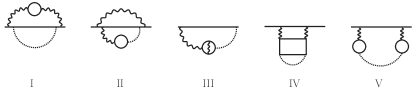
Figure 1: The different sets of vacuum polarization diagrams. Each set represents the drawn diagram plus all the possible permutations of its pieces.

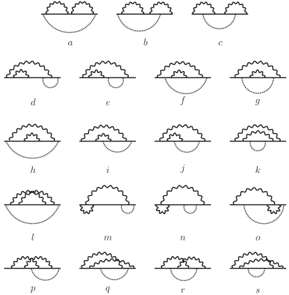
Figure 2: The diagrams involving a two-loop electron self-interaction and vertex corrections.

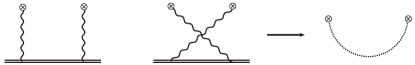
Figure 3: The sum of the direct and crossed diagrams is approximated by an effective propagator (the double line represents the propagator of the nucleus).

Since we are considering free asymptotic states with independent spins, the Dirac structures of the electron and the nucleus factorize, and we simplify them by inserting each of the structures between the spinors of the initial and final states and averaging over the spins of the initial states.

We use the program qgraf Nogueira:1991ex to generate all of the diagrams, and the packages q2e and exp Harlander:1997zb ; Seidensticker:1999bb to express them as a series of vertices and propagators that can be read by the FORM Vermaseren:2000nd package MATAD 3 Steinhauser:2000ry . Finally, MATAD 3 is used to represent the diagrams in terms of a set of scalar integrals using custom-made routines. In this way, we come to represent the amplitude $\mathcal{M}$ in terms of about 18000 different scalar integrals. These integrals can be expressed in terms of a few master integrals by means of integration-by-parts (IBP) identities Chetyrkin:1981qh . Using the so-called Laporta algorithm Laporta:1996mq ; Laporta:2001dd as implemented in the Mathematica package FIRE Smirnov:2008iw , we find 32 master integrals.

Since the program FIRE deals only with standard propagators, when using it we worked only with one of the nucleus propagators, instead of the Dirac delta of the effective propagator. That is, instead of working with $\delta(k^{0})$, we worked with $1/(2k\cdot N+i\epsilon)$, for example. Working with just one of the propagators is enough for this purpose, as the IBP method is insensitive to the $i\epsilon$ prescription (remember from Eq. (II) that in our approximation this is the only difference between the two propagators). Since each diagram in Figs. 1 and 2 represents the subtraction of two integrals that only differ in the nucleon propagator, when applying the IBP method we can set to zero any resulting integral in which the propagator $1/(2k\cdot N+i\epsilon)$ disappears. This can be done because the same integral with the propagator $1/(2k\cdot N-i\epsilon)$ instead would give the exact same contribution and thus the difference between the two is zero. Once the reduction to master integrals is complete, we can simply substitute back the delta function in place of the nucleon propagator.

In order to calculate the master integrals, we turned the expressions in Appendix A into a representation in terms of Feynman parameters. The procedure we then followed in most cases was to use a Mellin-Barnes representation Smirnov:1999gc ; Tausk:1999vh to break up sums of Feynman parameters raised to non-integer powers and transform the integrals into integrals of Gamma functions over the imaginary axis. In some cases, we were able to obtain analytical results. Otherwise, we used the Mathematica packages MB Czakon:2005rk and MBresolve Smirnov:2009up to perform a numerical calculation.

For integrals $I_{9}$, $I_{10}$, $I_{14}$, $I_{15}$, $I_{27}$, $I_{28}$, $I_{31}$, and $I_{32}$ (cf. Appendix A), the Mellin-Barnes representation was too cumbersome for a numerical evaluation. In these cases we used the Mathematica package FIESTA 1.2.1 Smirnov:2008py with integrators from the CUBA library Hahn:2004fe to perform numerical computations using sector decomposition Binoth:2000ps ; Heinrich:2008si . Like FIRE, FIESTA can only process standard propagators as input. This means that we had to use the momentum representation of the integrals with the nucleon propagators instead of the delta function. We separately calculated the integrals containing $1/(2N\cdot k+i\epsilon)$ and the ones containing $1/(-2N\cdot k+i\epsilon)$ instead, and added the two results. We checked the method by computing with FIESTA some integrals we had already found with MB and MBresolve. The results always agreed.

There was one case, integral $I_{32}$, where the FIESTA result for the integral with $1/(-2N\cdot k+i\epsilon)$ was numerically unstable. Fortunately, in this case we could find a representation in terms of Feynman parameters that we could compute directly using CUBA, without further treatment. This was possible because the integral is finite, and the representation was free of spurious divergences. We cross-checked this result using a beta version of FIESTA 2 Smirnov:2009pb , which did not produce the instabilities we encountered in the former version.

We performed an additional cross-check of our results by changing the basis of integrals. To do this, we took one of the integrals we computed with FIESTA and used the IBP method to express it in terms of a similar integral of our choice (same as the original one, but with some propagator(s) raised to different powers) plus other master integrals we already knew. We then computed the new integral with FIESTA and checked if the final result for the Lamb shift (or for individual diagrams) agreed with the calculation in the old basis. Since changing the basis modifies the coefficients of all the integrals involved in the change, the agreement of the results obtained with different bases is a very good cross-check of our calculations.

This cross-check was performed for several integrals. In particular, we changed integrals $I_{19}$ and $I_{27}$, which are the ones limiting our precision, and integrals $I_{15}$ and $I_{32}$. Since the last two integrals contain most of the propagators for integral types $F$ and $G$, the corresponding changes of basis affect the coefficients of most of the other integrals of the respective type.

III Results

Our final results for the separate contributions from the vacuum-polarization diagrams of Fig. 1 and the diagrams $a$–$s$ of Fig. 2 are

$$\delta E_{vac.} = \frac{\alpha^{2}(Z\alpha)^{5}}{\pi n^{3}}\left(\frac{\mu}{m}\right)^{3}m\,[0.86281422(3)]\,,$$ (3)

$$\delta E_{a-s} = \frac{\alpha^{2}(Z\alpha)^{5}}{\pi n^{3}}\left(\frac{\mu}{m}\right)^{3}m\,[-7.72381(4)]\,.$$ (4)

The best results so far for the vacuum polarization diagrams and for diagrams $a$–$s$ have been published in Pachucki:1993zz (cf. Eides:2000xc for references of partial results) and Eides:1995ey , respectively. Our results are compatible with them and improve the precision by two orders of magnitude in the case of $\delta E_{vac.}$ and a little over one order of magnitude for $\delta E_{a-s}$.

The total result reads

$$\delta E=\frac{\alpha^{2}(Z\alpha)^{5}}{\pi n^{3}}\left(\frac{\mu}{m}\right)^{3}m\,[-6.86100(4)]\,,$$ (5)

and the corresponding energy shifts for the $1S$ and the $2S$ states in hydrogen are

$$\delta E_{1S} = -296.866(2)\,\text{kHz}\,,$$ (6)

$$\delta E_{2S} = -37.1082(3)\,\text{kHz}\,.$$ (7)

Table 1: Comparison between our results for the different vacuum-polarization sets (in Fried-Yennie gauge) and those of Pachucki:1993zz ; Eides:1996uj . Numbers ending in an ellipsis indicate an analytic result, which we show in Appendix B.

Set	This paper	Refs. Pachucki:1993zz ; Eides:1996uj
I	$-0.07290996446926(4)$	$-0.0729098(3)$
II	0.61133839226…	$0.61133839226\dots$
III	0.50814858506…	$0.50814858506\dots$
IV	$-0.12291623(3)$	$-0.122915(3)$
V	$-23/378$	$-23/378$

Table 2: Comparison between our results for diagrams $a$–$s$ (in Fried-Yennie gauge) and those of Eides:1995ey . Numbers ending in an ellipsis indicate an analytic result, which we show in Appendix B.

Diagram	This paper	Ref. Eides:1995ey
$a$	0	0
$b$	2.955090809…	2.9551(1)
$c$	$-2.22312657\dots$	$-2.2231(1)$
$d$	$-5.2381153272259(2)$	$-5.238023(56)$
$e$	5.0561650638185(4)	5.056278(81)
$f$	$6\ln 2-207/40$	$-1.016145(21)$
$g$	$6\ln 2-147/80-\pi^{2}/4$	$-0.1460233(52)$
$h$	153/80	153/80
$i$	$-5.51731(2)$	$-5.51683(34)$
$j$	$-7.76838(1)$	$-7.76815(17)$
$k$	1.9597582447795(2)	1.959589(33)
$l$	1.74834(4)	1.74815(38)
$m$	1.87510512(6)	1.87540(17)
$n$	$-1.30570289(7)$	$-1.30584(18)$
$o$	$-12.06904(9)$	$-12.06751(47)$
$p$	6.13815(1)	6.13776(25)
$q$	$-7.52425(2)$	$-7.52453(34)$
$r$	14.36962(7)	14.36733(44)
$s$	$-0.9304766935602(5)$	$-0.930268(72)$

Choosing the Fried-Yennie gauge Fried:1958zz ; Adkins:1993qm , we also compared the results from the different sets of vacuum polarization diagrams with those of Pachucki:1993zz ; Eides:1996uj , and the results from the individual diagrams $a$–$s$ with those of Eides:1995ey . Our results for the vacuum polarization graphs and diagrams $a$–$s$ are presented in Tables 1 and 2, respectively. All numbers in the tables are to be multiplied by the prefactor $\alpha^{2}(Z\alpha)^{5}/(\pi n^{3})(\mu/m)^{3}m$ (note the difference in normalization in Pachucki:1993zz ).

We found new analytic results for four diagrams. The results for diagrams $f$ and $g$ are given in Table 2, while the results for diagrams $b$ and $c$, being too lengthy for the table, are presented in Appendix B. For completeness, the known analytic results for sets II and III of the vacuum polarization diagrams are given in Appendix B as well.

It should be mentioned that the errors of the results in Eqs. (3), (4), and (5) are not obtained from the sum of the errors of the diagrams in Tables 1 and 2. Once we decompose the problem into the calculation of master integrals, the diagrams are no longer independent, as the same master integral contributes to several different diagrams. Thus, to find the error of our total result, we first sum all diagrams and then sum all the errors of the integrals in quadrature.

We found discrepancies between our results for diagrams $a$–$s$ and those of Eides:1995ey . Most of the central values in the second and third column of table 2 lie between $1\sigma$ and $2\sigma$ away from each other, but in the case of diagrams $o$ and $s$ the difference is around $3\sigma$, and for diagrams $k$ and $r$, it reaches $5\sigma$ (we take as $\sigma$ the errors of individual diagrams in the third column). We should stress again that our calculation is done using dimensional regularization while the study of Ref. Eides:1995ey was performed in four dimensions. Even though all the individual diagrams are finite, one can imagine situations where the two regularization methods give different partial results. However, we do not observe significant cancellations in the sum of the differences. Thus, it seems the differences are real although practically negligible; their sum is very small and amounts to $10^{-3}$, which is the error estimate in Eides:1995ey . Thus our results agree within that error.

IV Summary

We have applied particle theory methods to compute, in dimensional regularization and a general covariant gauge, the corrections of order $\alpha^{2}(Z\alpha)^{5}$ to the Lamb shift. We have made use of IBP techniques to reduce the problem of computing all the necessary Feynman diagrams to the simpler problem of computing 32 scalar integrals. Mellin-Barnes integral representations and sector decomposition have then allowed us to obtain analytic results for some of these integrals, and good numerical results for the rest. With this, we have been able to reproduce and improve the results from previous calculations. The techniques used here are quite general and can be applied to other multi-loop problems in atomic physics.

Appendix A Results for the master integrals

In section II we presented our method of calculating the corrections to the Lamb shift, which differs significantly from the methods used in previous calculations. One important difference is the reduction of diagrams to master integrals. Here we present our results for all master integrals.

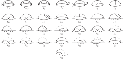
Figure 4: A graphic representation of the 32 master integrals. Solid and dashed lines represent massive and massless scalar propagators, respectively. The dotted double line denotes the delta function. A dot on a line signifies that the propagator is raised to a higher power. The external lines indicate the momentum $p$ of the electron flowing in and out of the diagram. The first two diagrams represent different integrals that differ only by a term in the numerator.

The set of master integrals is represented in Fig. 4. We have two different types of integrals. In Euclidean space, they are defined as:

$$F(\nu_{1},\nu_{2},\nu_{3},\nu_{4},\nu_{5},\nu_{6},\nu_{7},\nu_{8})=\frac{e^{3\gamma_{E}\epsilon}}{\left(\pi^{D/2}\right)^{3}}\int\frac{d^{D}k_{1}\,d^{D}k_{2}\,d^{D}k_{3}\;2\pi\,\delta(k_{2}^{0})}{(k_{1}^{2})^{\nu_{1}}\,(k_{2}^{2})^{\nu_{2}}\,(k_{3}^{2})^{\nu_{3}}\,[(k_{1}+p)^{2}+1]^{\nu_{4}}}$$

$$\times\frac{1}{[(k_{1}+k_{2}+p)^{2}+1]^{\nu_{5}}\,[(k_{1}+k_{2}+k_{3}+p)^{2}+1]^{\nu_{6}}\,[(k_{2}+k_{3}+p)^{2}+1]^{\nu_{7}}\,[(k_{3}+p)^{2}+1]^{\nu_{8}}}\,,$$ (8)

$$G(\nu_{1},\nu_{2},\nu_{3},\nu_{4},\nu_{5},\nu_{6},\nu_{7})=\frac{e^{3\gamma_{E}\epsilon}}{\left(\pi^{D/2}\right)^{3}}\int\frac{d^{D}k_{1}\,d^{D}k_{2}\,d^{D}k_{3}\;2\pi\,\delta(k_{1}^{0})}{(k_{1}^{2})^{\nu_{1}}\,(k_{2}^{2})^{\nu_{2}}\,(k_{3}^{2})^{\nu_{3}}\,[(k_{1}+k_{2}+p)^{2}+1]^{\nu_{4}}}$$

$$\times\frac{1}{[(k_{1}+k_{2}+k_{3}+p)^{2}+1]^{\nu_{5}}\,[(k_{2}+k_{3}+p)^{2}+1]^{\nu_{6}}\,[(k_{3}+p)^{2}+1]^{\nu_{7}}}\,,$$ (9)

where $D=4-2\epsilon$, and $p=(i,\vec{0})$ is the momentum of the electron. The mass of the electron has been set equal to one for convenience and can be easily restored from the dimension of the integral. The factor $e^{3\gamma_{E}\epsilon}$, where $\gamma_{E}$ is the Euler-Mascheroni constant, has been introduced to suppress the dependence of the results on this constant.

With these definitions, our results for the master integrals are:

$$I_{1} = F(1,0,0,0,0,1,0,1)=2e^{3\gamma_{E}\epsilon}\,\frac{\Gamma(1-\epsilon)\Gamma^{2}\left(-\frac{3}{2}+2\epsilon\right)\Gamma\left(-\frac{1}{2}+\epsilon\right)\Gamma\left(-\frac{5}{2}+3\epsilon\right)}{\Gamma(-3+4\epsilon)}\,,$$ (10)

$$I_{2} = F(1,0,-1,0,0,1,0,1)=-2I_{1}\,,$$ (11)

$$I_{3} = F(0,0,0,0,1,1,1,0)=-96.174642407742494299(1)-3003.97283051743374945(1)\epsilon$$ (12)

$$-16370.644886761701890(1)\epsilon^{2}-204040.09217878970569(1)\epsilon^{3}+\mathcal{O}(\epsilon^{4})\,,$$

$$I_{4} = F(-1,0,0,1,0,1,0,1)=128.23285654365665907(1)+4005.2971073565783326(1)\epsilon$$ (13)

$$+21827.526515682269186(1)\epsilon^{2}+272053.45623838627426(1)\epsilon^{3}+\mathcal{O}(\epsilon^{4})\,,$$

$$I_{5} = F(0,-1,0,0,1,1,1,0)=213.37528929773859515(1)-1789.0076495990746772(1)\epsilon+\mathcal{O}(\epsilon^{2})\,,$$ (14)

$$I_{6} = F(1,0,1,0,0,1,0,0)=2\sqrt{\pi}e^{3\gamma_{E}\epsilon}\,\frac{\Gamma^{2}(1-\epsilon)\Gamma\left(-\frac{5}{2}+3\epsilon\right)\Gamma\left(-\frac{3}{2}+2\epsilon\right)\Gamma\left(\frac{9}{2}-5\epsilon\right)}{\Gamma(2-2\epsilon)\Gamma(3-3\epsilon)}\,,$$ (15)

$$I_{7} = F(1,0,0,0,1,0,0,1)=2\sqrt{\pi}e^{3\gamma_{E}\epsilon}\,\frac{\Gamma(-1+\epsilon)\Gamma\left(-\frac{3}{2}+2\epsilon\right)\Gamma\left(\frac{5}{2}-3\epsilon\right)\Gamma(-\frac{1}{2}+\epsilon)}{\Gamma(2-2\epsilon)}\,,$$ (16)

$$I_{8} = F(0,0,0,0,1,0,1,1)=2\sqrt{\pi}e^{3\gamma_{E}\epsilon}\,\frac{\Gamma(-1+\epsilon)\Gamma\left(-\frac{3}{2}+2\epsilon\right)\Gamma^{2}\left(-\frac{1}{2}+\epsilon\right)}{\Gamma(-1+2\epsilon)}\,,$$ (17)

$$I_{9} = F(0,1,0,0,1,1,1,1)=-\frac{8\pi^{2}}{\epsilon}-257.35053226188(1)-2952.9668342496406(4)\epsilon+\mathcal{O}(\epsilon^{2})\,,$$ (18)

$$I_{10} = F(0,0,0,1,1,1,1,1)=-420.49901(1)+1860.837(4)\epsilon+\mathcal{O}(\epsilon^{2})\,,$$ (19)

$$I_{11} = F(1,0,0,0,1,1,0,1)=2^{3-4\epsilon}\pi e^{3\gamma_{E}\epsilon}\,\frac{\Gamma\left(\epsilon-\frac{1}{2}\right)}{\cos\left(2\pi\epsilon\right)}\left[2\frac{\Gamma\left(\frac{5}{2}-3\epsilon\right)\Gamma\left(\epsilon\right)}{\Gamma\left(4-4\epsilon\right)}\,{}_{3}F_{2}\left(1,\frac{5}{2}-3\epsilon,\epsilon;\frac{3}{2},4-4\epsilon;1\right)\right.$$ (20)

$$\left.-\sqrt{\pi}\frac{\Gamma\left(1-\epsilon\right)\Gamma\left(3\epsilon-\frac{3}{2}\right)}{\Gamma\left(\frac{5}{2}-2\epsilon\right)\Gamma\left(2\epsilon\right)}\,{}_{3}F_{2}\left(1,1-\epsilon,3\epsilon-\frac{3}{2};\frac{5}{2}-2\epsilon,2\epsilon;1\right)\right]\,,$$

$$I_{12} = F(1,1,0,0,1,1,0,1)=-\frac{4\pi^{2}}{\epsilon}-24\pi^{2}-\frac{4\pi^{4}}{3}+\pi^{2}\left(-116-\frac{59}{3}\pi^{2}+32\ln 2+100\zeta(3)\right)\epsilon+\mathcal{O}(\epsilon^{2})\,,$$ (21)

$$I_{13} = F(1,1,0,1,0,1,0,1)=-263.74028719521945979(1)+1741.1125810306205720(1)\epsilon+\mathcal{O}(\epsilon^{2})\,,$$ (22)

$$I_{14} = F(1,0,0,0,1,1,1,1)=-362.8560(1)+\mathcal{O}(\epsilon)\,,$$ (23)

$$I_{15} = F(1,1,0,0,1,1,1,1)=36.969282(2)+\mathcal{O}(\epsilon)\,,$$ (24)

$$I_{16} = F(1,4,0,0,1,0,1,1)=\pi^{2}\left(-\frac{513}{128\epsilon}-\frac{11077}{768}-\frac{571}{16}\ln 2+32\sqrt{5}\ln\left(\frac{1+\sqrt{5}}{2}\right)\right)$$ (25)

$$-1889.3810189605726842(1)\epsilon-2199.2559561980712031(1)\epsilon^{2}+\mathcal{O}(\epsilon^{3})\,,$$

$$I_{17} = F(1,0,0,0,2,0,2,1)=\frac{32\pi^{2}}{\sqrt{5}}\ln\left(\frac{1+\sqrt{5}}{2}\right)-683.43054120051764110(1)\epsilon$$ (26)

$$+5647.2496334930969112(1)\epsilon^{2}+\mathcal{O}(\epsilon^{3})\,,$$

$$I_{18} = F(1,4,1,0,1,0,1,1)=\pi^{2}\left[\frac{343}{512\epsilon}+\frac{125257}{46080}-\frac{2}{3}\pi^{2}+\frac{169}{192}\ln 2+16\ln^{2}2-48\ln^{2}\left(\frac{1+\sqrt{5}}{2}\right)\right]+\mathcal{O}(\epsilon)\,,$$ (27)

$$I_{19} = F(1,0,1,0,1,1,1,0)=-293.4480(2)+\mathcal{O}(\epsilon)\,,$$ (28)

$$I_{20} = F(1,0,0,1,1,0,1,1)=\pi^{2}\left[-\frac{2}{\epsilon}-2-\frac{8}{3}\pi^{2}+16\sqrt{5}\ln\left(\frac{1+\sqrt{5}}{2}\right)+32\ln^{2}\left(\frac{1+\sqrt{5}}{2}\right)\right]$$ (29)

$$+1394.0754186124348755(1)\epsilon+\mathcal{O}(\epsilon^{2})\,,$$

$$I_{21} = F(1,1,1,0,0,1,0,1)=2\pi^{2}-\frac{4\pi^{4}}{3}+\pi^{2}\left(44-4\pi^{2}+80\zeta(3)\right)\epsilon+\mathcal{O}(\epsilon^{2})\,,$$ (30)

$$I_{22} = F(0,0,0,1,1,0,1,1)=-\frac{128\pi^{2}}{3}-\pi^{2}\left(\frac{1792}{3}+\frac{256}{3}\pi-\frac{1024}{3}\ln 2\right)\epsilon+\mathcal{O}(\epsilon^{2})\,,$$ (31)

$$I_{23} = F(1,0,1,0,1,0,1,0)$$ (32)

$$= \frac{2\pi^{3}e^{3\gamma_{E}\epsilon}\,}{\Gamma^{2}\left(2-2\epsilon\right)\Gamma\left(\frac{3}{2}-\epsilon\right)}\left[2^{2\epsilon-2}\frac{\Gamma\left(1-\epsilon\right)\Gamma\left(\epsilon-\frac{1}{2}\right)}{\sin\left(\pi\epsilon\right)\cos\left(4\pi\epsilon\right)}\left(\frac{\Gamma\left(\frac{7}{2}-5\epsilon\right)\sin\left(\pi\epsilon\right)}{\Gamma\left(\frac{5}{2}-3\epsilon\right)\sin\left(2\pi\epsilon\right)\cos\left(3\pi\epsilon\right)}-\frac{\Gamma\left(3\epsilon-\frac{3}{2}\right)}{\Gamma\left(5\epsilon-\frac{5}{2}\right)\cos\left(2\pi\epsilon\right)}\right)\right.$$

$$+\frac{\sqrt{\pi}\,\Gamma\left(2-2\epsilon\right)\Gamma\left(2\epsilon-\frac{1}{2}\right)}{\Gamma\left(2-\epsilon\right)\Gamma\left(3\epsilon-\frac{1}{2}\right)\sin\left(\pi\epsilon\right)\cos\left(\pi\epsilon\right)\cos\left(3\pi\epsilon\right)}\,{}_{3}F_{2}\left(1,2-2\epsilon,2\epsilon-\frac{1}{2};2-\epsilon,3\epsilon-\frac{1}{2};1\right)$$

$$\left.-\frac{2^{1-2\epsilon}\pi\,\Gamma\left(\frac{5}{2}-3\epsilon\right)}{\Gamma\left(\frac{5}{2}-2\epsilon\right)\Gamma\left(\frac{1}{2}+\epsilon\right)\sin\left(2\pi\epsilon\right)\cos\left(\pi\epsilon\right)\cos\left(2\pi\epsilon\right)}\,{}_{3}F_{2}\left(1,\frac{5}{2}-3\epsilon,\epsilon;\frac{5}{2}-2\epsilon,2\epsilon;1\right)\right]\,,$$

$$I_{24} = G(0,1,2,1,0,1,0)=\frac{2\pi^{2}}{\epsilon}-162.745878930257(1)+640.681562239(2)\epsilon$$ (33)

$$-9490.745115169417(3)\epsilon^{2}+\mathcal{O}(\epsilon^{3})\,,$$

$$I_{25} = G(2,1,1,1,0,1,0)=-\frac{4\pi^{2}}{\epsilon}-192.3546921335253(1)-2297.18352848038(1)\epsilon$$ (34)

$$-10356.58582995624(1)\epsilon^{2}+\mathcal{O}(\epsilon^{3})\,,$$

$$I_{26} = G(1,1,1,1,0,1,0)=-\frac{4\pi^{2}}{\epsilon}-244.4995291143211(3)-2339.54007847666(2)\epsilon+\mathcal{O}(\epsilon^{2})\,,$$ (35)

$$I_{27} = G(0,1,1,2,0,1,1)=136.8086023(2)-907.048(2)\epsilon+\mathcal{O}(\epsilon^{2})\,,$$ (36)

$$I_{28} = G(0,1,1,1,1,1,0)=-280.62418(1)+734.494(1)\epsilon+\mathcal{O}(\epsilon^{2})\,,$$ (37)

$$I_{29} = G(1,1,1,0,1,1,1)=118.63826101784(1)+\mathcal{O}(\epsilon)\,,$$ (38)

$$I_{30} = G(0,1,1,0,1,1,0)=-10\sqrt{\pi}e^{3\gamma_{E}\epsilon}\,\frac{\Gamma\left(\epsilon\right)\Gamma^{2}\left(1-\epsilon\right)\Gamma\left(\frac{5}{2}-5\epsilon\right)\Gamma\left(-\frac{3}{2}+3\epsilon\right)}{\Gamma\left(2-2\epsilon\right)\Gamma\left(\frac{7}{2}-4\epsilon\right)}$$ (39)

$$\times{}_{3}F_{2}\left(\frac{7}{2}-5\epsilon,\frac{3}{2}-\epsilon,-\frac{1}{2}+\epsilon;\frac{7}{2}-4\epsilon,\frac{1}{2}+\epsilon;1\right)\,,$$

$$I_{31} = G(1,1,1,1,1,1,0)=49.3616(1)+\mathcal{O}(\epsilon)\,,$$ (40)

$$I_{32} = G(1,1,1,1,1,1,1)=26.272804(6)+291.1097(1)\epsilon+\mathcal{O}(\epsilon^{2})\,,$$ (41)

where $\zeta$ denotes Riemann’s zeta function, and ${}_{3}F_{2}$ is a generalized hypergeometric function. The latter can be expanded in $\epsilon$ with the help of the Mathematica package HypExp 2 Huber:2007dx .

The relation between integrals $I_{1}$ and $I_{2}$ expressed in Eq. (11) is not evident when looking at their respective representations. This relation becomes clear when checking the cancellation of the gauge-parameter dependence in the sum of all diagrams. If the 32 integrals presented here were an irreducible basis, the gauge dependence of the coefficient of each integral should vanish independently. However, this does not happen with the coefficients of integrals $I_{1}$ and $I_{2}$, which means that the integrals are connected. Demanding the cancellation of the gauge dependence yields Eq. (11). We checked this relation by computing explicitly the analytic solution for $I_{2}$.

There appears to be also a relation between integrals $I_{3}$ and $I_{4}$, although the gauge dependence does not give us any hint in this case. By demanding the cancellation of poles in several diagrams, one can find the following relation between the first three terms of $I_{3}$ and $I_{4}$,

$$I_{4}=-\frac{4}{3}I_{3}+\mathcal{O}(\epsilon^{3})\,.$$ (42)

The relation, however, seems to be valid to all orders in the $\epsilon$ expansion. We checked it numerically up to order $\epsilon^{4}$, but we could not find an analytic proof for it.

Integrals $I_{3}$–$I_{5}$, $I_{12}$, $I_{13}$, $I_{16}$, $I_{17}$, and $I_{20}$–$I_{22}$ can be represented as a one-fold Mellin-Barnes integral. We only show numerical results with 20-digit precision, which is more than enough for our purposes. However, these integrals can be easily evaluated with a precision of 100 digits or more. With this kind of precision it is possible to find analytical results, using the PSLQ algorithm pslq . In this way, we determined the $\mathcal{O}(\epsilon)$ term of integrals $I_{12}$ and $I_{21}$.

The analytic expression for the $\mathcal{O}(\epsilon^{0})$ term in $I_{20}$ was obtained using the analytic result for set II of vacuum-polarization diagrams presented in Eides:1996uj . Likewise, the analytic expression for the $\mathcal{O}(\epsilon)$ term in $I_{22}$ was extracted from the analytic result for set III found in Pachucki:1993zz . As mentioned above, we were able to numerically calculate these integrals to 100-digit precision and confirm the analytic expressions with PSLQ.

Appendix B Analytic results

Here we show the analytic results for diagrams $b$ and $c$ from Fig. 2:

$$\text{Diagram }b=$$ (43)

$$\frac{111}{8}-\pi^{2}-9\ln 2+24\ln^{2}2+\frac{48}{\sqrt{5}}\ln\left(\frac{1+\sqrt{5}}{2}\right)$$

$$-72\ln^{2}\left(\frac{1+\sqrt{5}}{2}\right),$$

$$\text{Diagram }c=$$ (44)

$$-\frac{352897}{27000}+\frac{31}{45}\pi^{2}-\frac{643}{225}\ln 2-\frac{248}{15}\ln^{2}2$$

$$+\frac{104}{9\sqrt{5}}\ln\left(\frac{1+\sqrt{5}}{2}\right)+\frac{248}{5}\ln^{2}\left(\frac{1+\sqrt{5}}{2}\right).$$

For completeness, we also give here the analytic results for sets II and III of the vacuum polarization diagrams, found in Eides:1996uj and Pachucki:1993zz , respectively:

Set II $$= \frac{67282}{6615}-\frac{2}{9}\pi^{2}+\frac{628}{63}\ln 2$$

$$-\frac{872}{63}\sqrt{5}\ln\left(\frac{1+\sqrt{5}}{2}\right)+\frac{8}{3}\ln^{2}\left(\frac{1+\sqrt{5}}{2}\right)\,,$$

Set III $$= \frac{15647}{13230}-\frac{25}{63}\pi+\frac{52}{63}\ln 2\,.$$ (46)

References

• (1) D. J. Berkeland, E. A. Hinds and M. G. Boshier, Phys. Rev. Lett. 75, 2470 (1995).
• (2) M. Weitz et al., Phys. Rev. A 52, 2664 (1995).
• (3) S. Bourzeix et al., Phys. Rev. Lett. 76, 384 (1996).
• (4) T. Udem, A. Huber, B. Gross, J. Reichert, M. Prevedelli, M. Weitz and T. W. Hänsch, Phys. Rev. Lett. 79, 2646 (1997).
• (5) C. Schwob et al., Phys. Rev. Lett. 82, 4960 (1999).
• (6) M. I. Eides, H. Grotch and V. A. Shelyuto, Phys. Rept. 342, 63 (2001) [arXiv:hep-ph/0002158].
• (7) K. Pachucki, Phys. Rev. A 63, 042503 (2001); M. I. Eides and V. A. Shelyuto, Can. J. Phys. 85, 509 (2007) [arXiv:physics/0612244].
• (8) K. Pachucki, Phys. Rev. A 53, 2092 (1996).
• (9) B. Lauss, Nucl. Phys. A 827, 401C (2009) [arXiv:0902.3231 [nucl-ex]]; A. Antognini et al., AIP Conf. Proc. 796, 253 (2005).
• (10) K. Pachucki, Phys. Rev. Lett. 72, 3154 (1994)
• (11) M. I. Eides and V. A. Shelyuto, Pisma Zh. Eksp. Teor. Fiz. 61, 465 (1995) [JETP Lett. 61, 478 (1995)].
• (12) M. I. Eides and V. A. Shelyuto, Phys. Rev. A 52, 954 (1995) [arXiv:hep-ph/9501303].
• (13) For a quantum field theoretical treatment of non-relativistic bound states see, for example, Sec. 5.3 of M. E. Peskin and D. V. Schroeder, Quantum Field Theory, (Westview Press, Boulder, 1995).
• (14) P. Nogueira, J. Comput. Phys. 105, 279 (1993).
• (15) R. Harlander, T. Seidensticker and M. Steinhauser, Phys. Lett. B 426, 125 (1998) [arXiv:hep-ph/9712228].
• (16) T. Seidensticker, arXiv:hep-ph/9905298.
• (17) J. A. M. Vermaseren, arXiv:math-ph/0010025.
• (18) M. Steinhauser, Comput. Phys. Commun. 134, 335 (2001) [arXiv:hep-ph/0009029]; URL: http://www-ttp.particle.uni-karlsruhe.de/~ms/software.html.
• (19) F. V. Tkachov, Phys. Lett. B 100, 65 (1981); K. G. Chetyrkin and F. V. Tkachov, Nucl. Phys. B 192, 159 (1981).
• (20) S. Laporta and E. Remiddi, Phys. Lett. B 379, 283 (1996) [arXiv:hep-ph/9602417].
• (21) S. Laporta, Int. J. Mod. Phys. A 15, 5087 (2000) [arXiv:hep-ph/0102033].
• (22) A. V. Smirnov, JHEP 0810, 107 (2008) [arXiv:0807.3243 [hep-ph]].
• (23) V. A. Smirnov, Phys. Lett.  B 460, 397 (1999) [arXiv:hep-ph/9905323].
• (24) J. B. Tausk, Phys. Lett.  B 469, 225 (1999) [arXiv:hep-ph/9909506].
• (25) M. Czakon, Comput. Phys. Commun. 175, 559 (2006) [arXiv:hep-ph/0511200].
• (26) A. V. Smirnov and V. A. Smirnov, Eur. Phys. J. C 62, 445 (2009) [arXiv:0901.0386 [hep-ph]].
• (27) A. V. Smirnov and M. N. Tentyukov, Comput. Phys. Commun. 180, 735 (2009) [arXiv:0807.4129 [hep-ph]].
• (28) T. Hahn, Comput. Phys. Commun. 168, 78 (2005) [arXiv:hep-ph/0404043].
• (29) T. Binoth and G. Heinrich, Nucl. Phys. B 585, 741 (2000) [arXiv:hep-ph/0004013]; Nucl. Phys. B 680, 375 (2004) [arXiv:hep-ph/0305234]; Nucl. Phys. B 693, 134 (2004) [arXiv:hep-ph/0402265].
• (30) G. Heinrich, Int. J. Mod. Phys. A 23, 1457 (2008) [arXiv:0803.4177 [hep-ph]].
• (31) A. V. Smirnov, V. A. Smirnov and M. Tentyukov, arXiv:0912.0158 [hep-ph].
• (32) K. Pachucki, Phys. Rev. A 48, 2609 (1993).
• (33) H. M. Fried and D. R. Yennie, Phys. Rev. 112, 1391 (1958).
• (34) G. S. Adkins, Phys. Rev. D 47, 3647 (1993).
• (35) M. I. Eides, H. Grotch and V. A. Shelyuto, Phys. Rev. A 55, 2447 (1997) [arXiv:hep-ph/9610443].
• (36) J. A. M. Vermaseren, Comput. Phys. Commun. 83, 45 (1994).
• (37) D. Binosi, J. Collins, C. Kaufhold and L. Theussl, Comput. Phys. Commun. 180, 1709 (2009) [arXiv:0811.4113 [hep-ph]].
• (38) T. Huber and D. Maître, Comput. Phys. Commun. 178, 755 (2008) [arXiv:0708.2443 [hep-ph]].
• (39) H.R.P. Ferguson, D.H. Bailey and S. Arno, Math. Comput. 68, 351 (1999).