Feature selection when there are many influential features

Abstract

Recent discussion of the success of feature selection methods has argued that focusing on a relatively small number of features has been counterproductive. Instead, it is suggested, the number of significant features can be in the thousands or tens of thousands, rather than (as is commonly supposed at present) approximately in the range from five to fifty. This change, in orders of magnitude, in the number of influential features, necessitates alterations to the way in which we choose features and to the manner in which the success of feature selection is assessed. In this paper, we suggest a general approach that is suited to cases where the number of relevant features is very large, and we consider particular versions of the approach in detail. We propose ways of measuring performance, and we study both theoretical and numerical properties of the proposed methodology.

, and

1 Introduction

1.1 Motivation and summary

In this paper, we develop statistical methods for determining features that enable effective discrimination between two populations of very high dimensional data, when the number of component-wise differences that provide leverage for discrimination is relatively large but the sizes of those differences are potentially small. By way of contrast, conventional approaches to solving this problem tend to rely on relatively large differences and relatively small numbers of components where differences occur.

In such problems, it is generally going to be of substantial practical interest to identify, with reasonable accuracy, the components that have greatest leverage for correct discrimination. Simply constructing a classifier, which might depend in a difficult-to-determine way on differences between two populations, is generally not going to provide all the information that is sought. However, particularly when the number of such components is large, we may not be able to identify the components without error. How accurate can we be, and in what circumstances is accuracy high? In this paper we shall endeavour to answer these questions.

Achieving reasonable accuracy can involve relatively computer-intensive methods, for example, algorithms that need $\mathrm{O}(p^{2})$ rather than $\mathrm{O}(p)$ time if the problem is $p$-dimensional. However, if we use an initial, deterministic dimension reduction step, which decreases dimension to $q$ where $q\ll p$, then $\mathrm{O}(p^{2})$ calculations can be reduced to $\mathrm{O}(p\log p+q^{2})$, where $p\log p$ is the computational cost of ordering the initial $p$ components. In many cases, we expect $q$ to be a rather crude upper bound to the true number, $r$ say, of components that impact on performance of the classifier. The four-stage algorithm that we shall introduce in Section 2 enables us to reduce computational expense from $\mathrm{O}(p\log p+q^{2})$ to $\mathrm{O}(p\log p+r^{2})$. (These order-of-magnitude calculations ignore the effects of training sample size, $n$ say, since in the problems we are considering $n$ is typically much less than $p$, $q$ or $r$ and so has relatively little impact on the final result.)

Support for the conjecture that $r$ can be quite large, for example, in genomics problems, has been given by Goldstein [29], who, in the words of J.N. Hirschhorn in the same issue of the New England Journal of Medicine, “builds a speculative mathematical model and infers that there will be tens of thousands of common variants influencing each disease and trait” (Hirschhorn [35]). Goldstein’s [29] calculations are also consistent with $r$ being in the thousands, not just the tens of thousands:

$\ldots$ the genetic burden of common diseases must be mostly carried by large numbers of rare variants. In this theory, schizophrenia, say, would be caused by combinations of 1000 rare genetic variants, not of 10 common genetic variants.

(See Wade [43].) Kraft and Hunter [37] argue that “many, rather than few, variant risk alleles are responsible for the majority of the inherited risk of each common disease.” Again, $r$ is large rather than small.

In the discussion above one might interpret $p$ and $r$ as representing numbers of single nucleotide polymorphisms (SNPs), alleles, or perhaps genes. There are believed to be between 10 and 30 million SNPs on a human chromosome, and some 25,000 genes. However, genomic analyses based on decoding the full DNA of individuals who suffer from specific conditions (Wade [43]) increase the values of both $p$ and $r$ by orders of magnitude. (In practice $r$ will be chosen empirically, and so will actually be a function of the data, but at the level of the discussion in the present section there is little to be gained by making this distinction.)

1.2 Example

We do not have to look beyond datasets well covered in the statistical literature to see evidence of a very large number of influential components being present in a dataset. We have taken three popular microarray datasets, described in more detail in Section 5.4, pertaining to colon cancer, leukemia and prostate cancer. In each case, there are many thousands of genes, each with a continuum of expression levels, as well as a binary response variable, indicating whether or not a patient carries the condition. For each dataset we performed a Wilcoxon rank sum test for each gene, using the response to divide observations, so as to test nonparametrically for a change in mean. The kernel estimates of the densities of $p$-values from these experiments are displayed in Figure 1 in solid red lines. The peak at the left for each dataset suggests a significant number of low $p$-values, more than would be expected if only a few genes contributed to the understanding of the response.

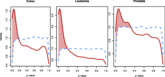
Figure 1: Distribution of $p$-values of Wilcoxon tests applied to the components of microarray datasets. The red solid line represents the actual data, while the dashed blue line is when the response is randomly permuted and so there is no genuine signal. The shaded regions give estimates of the proportion of components genuinely related to the response.

To extend the experiment further, we randomly permuted the response amongst the observations 50 times and repeated the Wilcoxon tests, recovering the distributions denoted by the blue dashed lines. These can be thought of as the expected distributions of $p$-values were each gene independently varying with respect to the response. They asymptotically approximate the uniform distribution. The shaded region in each plot then provides a rough estimate of the fraction of components related to the response. These fractions are 16%, 30% and 8.5% of all genes considered (or equivalently, 320, 2140 and 510 genes, resp.), for the colon, leukemia and prostate datasets, respectively. We have also done a similar experiment for a SNP data on multiple sclerosis to be introduced in Section 5.5, where the fraction is $3.9\%$ out of 300,900 SNPs. It should also be noted that these observations are genuine; the statistic measured (difference between estimated densities) is many standard deviations above what would be expected by chance.

1.3 Comments on the literature

Methods for feature selection based on the linear model are generally considered only in cases where the number of features is relatively small. Otherwise, the value of the response variable can be unreasonably insensitive to changes in a single feature. Examples of approaches founded on the linear model include the nonnegative garrotte (e.g., Breiman [6, 7]; Gao [27]), the lasso (Tibshirani [40]), the Dantzig selector (Candes and Tao [8]), and related techniques (e.g., Donoho and Huo [17]; Fan and Li [22, 23]; Donoho and Elad [16]; Tropp [42]; Donoho [14, 15]; Fan and Ren [25]; Fan and Fan [21]). The feature-ranking approach that we consider is more closely related to correlation-based approaches of Fan and Lv [24] and Hall and Miller [31], but it is does not assume the existence of a response variable. Instead it utilises class labels via a logistic model. Monograph-length treatments of classifiers and related methodology include those of Duda et al. [20], Hastie et al. [34] and Shakhnarovich et al. [38].

2 Methodology

2.1 Data and algorithm

Denote the two populations of interest by $\Pi_{0}$ and $\Pi_{1}$. Training data from each are acquired as $p$-vectors $X_{i}=(X_{i1},\ldots,X_{ip})$, for $1\leq i\leq n$. We also record the value of a label $I_{i}$, for each $i$; it equals 0 or 1, indicating the index of the population from which $X_{i}$ came.

One potential algorithm for identifying indices $j$, of vector components $X_{ij}$ which capture differences between $\Pi_{0}$ and $\Pi_{1}$, has four stages, (1)–(4) below. The goal of the algorithm is to determine empirically a set $\{{\hat{\jmath}}_{1},\ldots,{\hat{\jmath}}_{r}\}$ of indices, a subset of $\{1,\ldots,p\}$, such that the features with indices ${\hat{\jmath}}_{1},\ldots,{\hat{\jmath}}_{r}$ have significant influence on whether $X_{i}$ comes from $\Pi_{0}$ or $\Pi_{1}$. Those features can then be combined into a classifier, for example, the support vector machine or a centroid-based method, to effect discrimination.

(1) Component ranking. Using a method such as that suggested in Section 2.2, rank all components in terms of their individual influence on $I_{i}$, interpreted as a zero–one response variable. This stage takes $\mathrm{O}(p\log p)$ time to run, and produces a permutation ${\hat{\jmath}}_{1},\ldots,{\hat{\jmath}}_{p}$, say, of $1,\ldots,p$, where the order of the sequence ${\hat{\jmath}}_{1},\ldots,{\hat{\jmath}}_{p}$ is of major importance and signifies that, for each $k$, the component with rank ${\hat{\jmath}}_{k}$ has greater leverage than the component with rank ${\hat{\jmath}}_{k+1}$ on a measure of our ability to predict $I_{i}$ from $X_{i}$.

(2) Deterministic dimension reduction. Truncate at $q$ (where $1\leq q\leq p$) the sequence we derived in step (1). From this point, we work only with $q$-vectors comprised of the components with indices ${\hat{\jmath}}_{1},\ldots,{\hat{\jmath}}_{q}$. The value of $q$ is determined largely by our computational resources, bearing in mind that the computational expense of constructing the classifier could be as high as $\mathrm{O}(q^{2})$.

(3) Adaptive dimension reduction. In this stage, we use an empirical method to reduce dimension from $q$, chosen in stage (3), to $r$, so that the final choice of feature indices is ${\hat{\jmath}}_{1},\ldots,{\hat{\jmath}}_{r}$. Potential approaches are discussed in Section 2.3, and include methods based on: (3a) thresholding, (3b) change-point methods, or (3c) application of classifiers to blocks of components.

(4) Backing and filling. In practice, it can be advantageous to rerun stage (3) of the algorithm using several of the values of $j$ chosen early in stage (2), or early in the implementation of stage (3), bearing in mind that there is potential for noise in the choice of ${\hat{\jmath}}_{1}$, for example, to throw the algorithm off course for a period. At this point we could, for example, experiment with different choices of block size in method (3c).

2.2 Method for ranking components

Given an index $j$ between 1 and $p$, and scalar parameters $\alpha$ and $\beta$, we capture the relationship between $I_{i}$ and $X_{ij}$ by assuming a logit model:

$$P(I_{i}=0|X_{ij})=\bigl{\{}1+\exp(\alpha+\beta X_{ij})\bigr{\}}^{-1},\qquad P(I_{i}=1|X_{ij})=1-P(I_{i}=0|X_{ij}).$$

The likelihood of $I_{i}$, given $X_{ij}$, is

$$L_{ij}(I_{i}|\alpha,\beta;X_{ij})=\biggl{(}\frac{t_{ij}}{1+t_{ij}}\biggr{)}^{I_{i}}\biggl{(}\frac{1}{1+t_{ij}}\biggr{)}^{1-I_{i}}=\frac{t_{ij}^{I_{i}}}{1+t_{ij}},$$

where $t_{ij}=\exp(\alpha+\beta X_{ij})$. Therefore, the negative log-likelihood is

$$\ell_{ij}(\alpha,\beta)=-\log L_{ij}(I_{i}|\alpha,\beta;X_{ij})=-I_{i}(\alpha+\beta X_{ij})+\log\bigl{\{}1+\exp(\alpha+\beta X_{ij})\bigr{\}},$$ (1)

and its counterpart for $X_{1j},\ldots,X_{nj}$ is

$$\ell_{j}(\alpha,\beta)=\frac{1}{n}\sum_{i=1}^{n}\ell_{ij}(\alpha,\beta).$$ (2)

Define $({\hat{\alpha}}_{j},{\hat{\beta}}_{j})$ to be the value of $(\alpha,\beta)$ that minimises $\ell_{j}(\alpha,\beta)$, and put

$${\hat{\ell}}_{j}=\ell_{j}({\hat{\alpha}}_{j},{\hat{\beta}}_{j}).$$ (3)

The ordering ${\hat{\jmath}}_{1},\ldots,{\hat{\jmath}}_{p}$ mentioned in step (1) of the algorithm in Section 2.1 is determined by the values of ${\hat{\ell}}_{j}$. Specifically, ${\hat{\ell}}_{{\hat{\jmath}}_{1}}\leq\cdots\leq{\hat{\ell}}_{{\hat{\jmath}}_{p}}$.

2.3 Methods for adaptive dimension reduction

Several approaches are feasible, including: (3a) Thresholding. Here we compute, from the data, a subsidiary criterion ${\tilde{\ell}}_{j}$, for $1\leq j\leq p$ (we might simply choose ${\tilde{\ell}}_{j}\equiv 0$) and a threshold $t$; we take $k_{0}\geq 0$ to be an integer; and we define $r\in[k_{0}+1,q]$, a function of the data, to be the least integer in that range such that ${\hat{\ell}}_{{\hat{\jmath}}_{r+k}}-{\tilde{\ell}}_{{\hat{\jmath}}_{r+k}}>t$ for $1\leq k\leq k_{0}$. See Section 4 for an example. (3b) Change-point methods. Here we look for a change-point in the sequence ${\hat{\ell}}_{{\hat{\jmath}}_{1}},\ldots,{\hat{\ell}}_{{\hat{\jmath}}_{p}}$, and we take ${\hat{\jmath}}_{r}$ to be the location of that point. (There is a vast literature on methodology and theory for change-point detection. It includes book-length accounts by Carlstein et al. [9], Csörgő and Horváth [12], Chen and Gupta [11] and Wu [44].) (3c) Application of classifiers. For $k\geq 1$, let ${\mathcal{B}}_{k}=\{{\hat{\jmath}}_{(k-1)b+1},\ldots,{\hat{\jmath}}_{kb}\}$ denote the $k$th block of feature indices; here, $b$ denotes block length. (Theoretical considerations suggest that taking $b\sim\mathrm{const.}\ n$ is appropriate.) In step $s$ of stage (3c) we construct the classifier that is based on the training data vectors where all but the components with indices in $\bigcup_{1\leq k\leq s}{\mathcal{B}}_{k}$ have been stripped away. We use cross-validation to measure classifier performance, and in this way we determine whether progressing from step $s$ to step $s+1$ gives an improvement. If it does not then, subject to the “jiggling” suggested in stage (4), we stop at step $s$. If performance is improved by passing to the $(s+1)$st block then we proceed to step $s+1$, where we again assess performance. However, this approach can be biased in favour of low apparent error rate, without having the same impact on actual error rate; see Section 5.3 for discussion.

2.4 Duration of algorithm

Stage (3) of the algorithm takes $\mathrm{O}(r^{2})$ time to complete, where $r$, in the range $1\leq r\leq q$, denotes the final number of components on which we determine that the classifier should depend. In particular, the algorithm concludes with a list of $r$ components, say ${\hat{\jmath}}_{\ell_{1}},\ldots,{\hat{\jmath}}_{\ell_{r}}$ where $\{{\hat{\jmath}}_{\ell_{1}},\ldots,{\hat{\jmath}}_{\ell_{r}}\}=\bigcup_{k\leq{\hat{s}}}{\mathcal{B}}_{k}\subseteq\{{\hat{\jmath}}_{1},\ldots,{\hat{\jmath}}_{q}\}$, on which the final classifier is based. The $\mathrm{O}(r^{2})$ figure is derived as follows: Constructing the classifier from $s$ batches takes $\mathrm{O}(sb)$ time, so the total time needed is $\mathrm{O}(\sum_{1\leq s\leq{\hat{s}}}sb)=\mathrm{O}({\hat{s}}^{2}b)=\mathrm{O}(r^{2})$. Here, since $b$ is generally of order $n$ (see Section 5) and ${\hat{s}}^{2}b=\mathrm{O}(r^{2}b)$, we have replaced $r^{2}b$ by $r^{2}$ since, in the problems we are treating, $n$ is generally so much less than $r$ that it can be treated as fixed. Provided the number of reruns in stage (4) is only $\mathrm{O}(1)$, the order of magnitude of the time taken to run the algorithm to completion is $\mathrm{O}(p\log p+r^{2})$.

2.5 Discussion

The procedures above are intended to reflect methodologies already used in practice. Our main aim is to show that such techniques can be used to address not just contemporary problems where there is believed to be considerable sparsity and only a small number of significant features (e.g., five or ten genes out of thousands or tens of thousands), but also reduced sparsity and a larger total number of features (e.g., thousands or tens of thousands of DNA sequences out of tens or hundreds of thousands of possibilities). Additionally we show that the methods continue to work well under minimal distributional assumptions (e.g., normality is not needed), and minimal conditions about relationships among features. In all these senses, procedures such as those described above are particularly versatile.

The proposed approach belongs to the class of marginal methods for that it only uses marginal information for feature selection. Marginal methods are feasible when different features are independent or weakly dependent. When this is not the case, a natural problem is how to incorporate dependence among different features for feature ranking and classification. One possible approach is to first estimate the correlations and then include them in the classifier. However, without rather narrow assumptions this can introduce substantial noise into the process of inference for high-dimensional data, and in fact one can be better off simply ignoring the correlations; see, for example, Tibshirani et al. [41], Bickel and Levina [5] and Fan and Fan [21].

The feature ranking problem can also be re-cast in terms of logistic regression, where the design matrix $\{X_{ij}\}_{\{1\leq i\leq n,1\leq j\leq p\}}$ is randomly generated and perhaps non-Gaussian. Hence, there is a natural connection between the component-by-component, or marginal, approach suggested in the present paper, and existing techniques for feature selection, such as the lasso (e.g., Chen et al. [10]; Tibshirani [40]). Genovese et al. [28] compared marginal methods with the lasso and showed that the two approaches have comparable performance over a wide range of parameter values, both theoretically and empirically, but that marginal methods are computationally more efficient, especially when both $n$ and $p$ are large.

Our work is connected to that of Fan and Lv [24] in that it is founded on component-wise analysis of high-dimensional data. Fan and Lv’s ingenious technique was based on correlation, and is related to likelihood through its connections to least-squares in the setting of Gaussian experimental errors. In contrast, we use a logistic model to define a likelihood for each component, and we rank those component-wise likelihoods. Fan and Lv’s [24] aim is “to reduce dimensionality from high to a moderate scale that is below the sample size” (to quote from their paper), and then to use relatively conventional methods to select features. However, our goal is inherently different, since a basis for our argument is the concern that, as Goldstein [29] argued, the number of important features might be relatively large, and in particular much larger than sample size.

Our paper is connected to those of Fan and Lv [24] and Fan and Song [26], and in particular our methodology, minus the “adaptive dimension reduction” and “backing and filling” steps, is Fan and Song’s [26] SIS approach when the model in question is logistic. However, the parameter settings that we treat, both in our numerical work and our theory, are quite different from theirs. In particular, we focus on regimes where the useful features are very weak and only moderately sparse. In contrast, Fan and Lv [24] and Fan and Song [26] address cases where the signals are relatively strong or very sparse. Secondly, we evaluate our approach using the new criterion of misranking, introduced below, which is particularly appropriate to problems where many influential features are present and, for at least this reason, different from criteria employed by Fan and Lv [24] and Fan and Song [26]. It is also different from the FDR approach adopted by Benjamini and Hochberg [4] and many other authors.

In broad terms the methodology that we suggest could be used in conjunction with existing approaches to feature selection, but those generally do not conclude with a ranking of features, and that would limit their usefulness to us. More particularly, as discussed above, our approach differs from those of Fan and Lv [24] and others, in that our aim is not to dramatically reduce the number of features to a handful, but to address a much larger number of features. Nevertheless some methods, for example, random forests (which produce a feature importance list) and shrunken centroids do create an ordering for the portion of predictors that are given nonzero weight, and would be candidates for implementing part of our methodology.

3 Properties of feature ranking

3.1 Main result on ranking

Let $\pi=E(I_{i})$ denote the proportion of data that come from population $\Pi_{1}$. We assume below that $0<\pi<1$, and that when the training data are drawn randomly from the union of $\Pi_{0}$ and $\Pi_{1}$, the prior probability that any given datum $X_{i}$ is from $\Pi_{1}$ equals $\pi$. Therefore, the corresponding probability for $\Pi_{0}$ is $1-\pi$. We take $n$, representing the total size of the training sample, to be the key asymptotic parameter, and interpret the dimension, $p$, of $X_{i}$ as a function of $n$.

Next, we describe our model. Write $X_{i}=(X_{i1},\ldots,X_{ip})$, and, when $X_{i}$ comes from $\Pi_{1}$, take

$$X_{ij}=\mu_{j}+Z_{ij},$$ (4)

where $\mu_{j}\geq 0$ are constants and, for simplicity, we assume that the variables $Z_{ij}$ are identically distributed as $Z$, say. (This condition can be relaxed; see (8) below.) Take $X_{ij}=Z_{ij}$ when $X_{i}$ is drawn from $\Pi_{0}$. The vectors $(Z_{i1},\ldots,Z_{ip})$ and variables $I_{i}$, for $1\leq i\leq n$, are assumed to be totally independent. We allow the $\mu_{j}$’s to be functions of $n$.

Write ${\hat{\alpha}}_{j}$ and ${\hat{\beta}}_{j}$ for the values of $\alpha$ and $\beta$ that jointly minimise ${\hat{\ell}}_{j}(\alpha,\beta)$ within radius $n^{-c}$ of $(\alpha_{0},0)$, where $\alpha_{0}=\log\{\pi/(1-\pi)\}$, for any given $c\in(0,{{\frac{1}{2}}})$. (A separate argument can be used to prove that if ${\hat{\alpha}}_{j}$ and ${\hat{\beta}}_{j}$ are chosen without constraint then, under the conditions of Theorem 1 below, they satisfy ${\hat{\alpha}}_{j}=\alpha_{0}+\mathrm{O}_{p}(n^{-c})$ and ${\hat{\beta}}_{j}=\mathrm{O}_{p}(n^{-c})$ uniformly in $1\leq j\leq p$, for some $c\in(0,{{\frac{1}{2}}})$.) Define

$$S_{j}=\frac{\sum_{i}(I_{i}-\pi)X_{ij}}{n\pi(1-\pi)},$$ (5)

and note that $E(S_{j})=0$. Put $\lambda=(n^{-1}\log n)^{1/2}$.

Theorem 1

Assume that for each $n$, $|\mu_{j}|\leq\mathrm{const.}\ \lambda$ for $1\leq j\leq p$; that $p=p(n)\to\infty$ and, for constants $B_{1}>0$ and $B_{2}>2\max(B_{1}+3,2B_{1})$, $p=\mathrm{O}(n^{B_{1}})$ and $0<E|Z|^{B_{2}}<\infty$; and that $E(Z)=0$. Then, uniformly in $1\leq j\leq p$,

$${\hat{\ell}}_{j}=\ell_{j}({\hat{\alpha}}_{j},{\hat{\beta}}_{j})=R-{{{\textstyle\frac{1}{2}}}}\pi(3-2\pi)\bigl{(}EZ^{2}\bigr{)}^{-1}(S_{j}+\mu_{j})^{2}+\mathrm{O}_{p}\bigl{(}\lambda^{3}\bigr{)},$$ (6)

where the random variable $R=R(n)$ does not depend on $j$. More particularly, the $\mathrm{O}_{p}(\lambda^{3})$ term in (6) can be written as $\Theta_{j}\lambda^{3}$, where, for a constant $B_{3}$ depending on $B_{1}$ and $B_{2}$, and with $B_{4}={{\frac{1}{4}}}\{B_{2}-2\max(B_{1}+3,2B_{1})\}-\varepsilon$ for any $\varepsilon>0$, the random variables $\Theta_{j}$, for $1\leq j\leq p$, satisfy:

$$\sum_{j=1}^{p}P\bigl{(}|\Theta_{j}|>B_{3}\bigr{)}=\mathrm{O}\bigl{(}n^{-B_{4}}\bigr{)}$$ (7)

as $n\to\infty$.

The statistic $S_{j}$ is, up to normalisation, the well-known $z$-score statistic for testing whether the $j$th feature is significant or not; see, for example, Donoho and Jin [18, 19] and Jin [36]. In (6), since the first term, $R$, does not depend on $j$ then the second term is the one that reflects the strengths of individual features. As a result, ranking features according to ${\hat{\ell}}_{j}$ gives close, but not necessarily the same, results as ranking features according to $|S_{j}+\mu_{j}|$.

Next, we interpret the assumptions imposed in Theorem 1. The condition $|\mu_{j}|\leq\mathrm{const.}\ \lambda$, for $1\leq j\leq p$, is imposed so as to make the contribution of $\mu_{j}$ difficult to identify. In particular, if $|\mu_{j}|$ is of larger order than $\lambda$ then it can be shown from large deviation properties that the contribution of the “signal” $\mu_{j}$ will be easily visible above the noise, and so the contribution of the gene corresponding to the index $j$ will be very easy to identify. This would exemplify the classical setting, where a relatively small number of genes describe adequately the link to disease, and we are not addressing that case in this paper. The conditions $p=\mathrm{O}(n^{B_{1}})$ and $0<E|Z|^{B_{2}}<\infty$ imply that the number of dimensions can be polynomially large as a function of sample size, and that only a polynomial number of moments needs to be assumed. The assumption $B_{2}>2\max(B_{1}+3,2B_{1})$ implies that the number of moments required increases no faster than linearly as a function of the rate of growth of $p$, expressed in terms of sample size.

The assumption that each $Z_{ij}$ has the same distribution is made to simplify discussion and notation, and is readily relaxed. For example, it suffices to assume that each $Z_{ij}$, for $1\leq i\leq n$, is distributed as $Z_{j}$, say, where, instead of the assumptions imposed on $Z$ in the theorem, we ask that:

$$E(Z_{j})=0$$, is bounded away from zero and infinity uniformly in , and for all and some random variable , where .

(8)

In this case, the moment $E(Z^{2})$ in (6) would be replaced by $E(Z_{j}^{2})$. The conclusions that we draw, below, from Theorem 1 are unchanged, provided we interpret $\mu_{j}$ as $\mu_{j}/(EZ_{j}^{2})^{1/2}$ during discussion.

Although we ask that the vectors $X_{i}$ be independent, we make no assumption about the relationships among their components. For example, the values of $Z_{i1},\ldots,Z_{ip}$ can be highly dependent (indeed, in an extreme case, equal to one another) or completely independent. The latter instance is actually the most difficult, in terms of rigorously establishing that (6) and (7) hold. At the other end of the spectrum, the case where $Z_{i1}=\cdots=Z_{ip}$ with probability 1 is trivial, since there effectively only a single component index, with different candidate values for the mean, has to be treated.

3.2 Expected number of misrankings

Assume that some of the $\mu_{j}$’s are zero and all the others are strictly positive. Ideally, we would like the criterion ${\hat{\ell}}_{j}$ to be a good indicator of the positivity of $\mu_{j}$, in particular to take a lesser (or larger negative) value if $\mu_{j}$ is positive than it does when $\mu_{j}=0$. Reflecting this aspiration, if there exist component indices $j_{1}$ and $j_{2}$ such that $\mu_{j_{1}}>0$ and $\mu_{j_{2}}=0$, but ${\hat{\ell}}_{j_{2}}<{\hat{\ell}}_{j_{1}}$, then we shall say that a misranking has occurred. The expected total number of misrankings,

$$\nu_{\mathrm{misrank}}=\sum_{j_{1}\colon\ \mu_{j_{1}}>0}\sum_{j_{2}\colon\ \mu_{j_{2}}=0}P({\hat{\ell}}_{j_{2}}<{\hat{\ell}}_{j_{1}}),$$

is a measure of the performance of ${\hat{\ell}}_{j}$ as a criterion for distinguishing between positive and zero values of $\mu_{j}$; lower values of $\nu_{\mathrm{misrank}}$ correspond to higher performance.

Since the random variable $S_{j}$ in (5) and (6) has standard deviation of size $n^{-1/2}$ then, if the positive $\mu_{j}$’s are of smaller order than $n^{-1/2}$, with probability converging to ${{\frac{1}{2}}}$ any attempt to rank any pair of means $\mu_{j}$ using the values of ${\hat{\ell}}_{j}$ will produce the wrong result about half the time. The following theorem makes this clear. Let $p_{1}$ denote the number of indices $j$ for which $\mu_{j}>0$, and put

$$\sigma_{j_{1}j_{2},\pm}^{2}=\pi(1-\pi)\operatorname{var}(Z_{1j_{1}}\pm Z_{1j_{2}})$$ (9)

for respective choices of the plus and minus signs.

To avoid degeneracy, where the problem of identifying genes is relatively simple, we assume below that the quantities $\sigma_{j_{1}j_{2},\pm}^{2}$ are bounded away from zero, and of course, since we are endeavouring to capture cases where the signals $\mu_{j}$ are so weak that the corresponding genes cannot be identified, we ask that the $\mu_{j}$’s be uniformly of smaller order than $n^{-1/2}$.

Theorem 2

Assume the conditions of Theorem 1, that $\sup_{j\leq p}\mu_{j}=\mathrm{o}(n^{-1/2})$, and that $\sigma_{j_{1},j_{2},\pm}^{2}$ is bounded away from zero uniformly in $j_{1}$, $j_{2}$ and choices of the $\pm$ signs. Then $P({\hat{\ell}}_{j_{2}}<{\hat{\ell}}_{j_{1}})\to{{\frac{1}{2}}}$ uniformly in $1\leq j_{1},j_{2}\leq p$, in particular uniformly in pairs $j_{1},j_{2}$ such that $\mu_{j_{1}}>0$ and $\mu_{j_{2}}=0$. Moreover, $\nu_{\mathrm{misrank}}={{\frac{1}{2}}}p_{1}(p-p_{1})+\mathrm{o}\{p_{1}(p-p_{1})\}$ as $n\to\infty$.

Likewise, if the positive $\mu_{j}$’s are of size $n^{-1/2}$ then the probability of incorrectly ranking the $j_{1}$th component lower than the $j_{2}$th component, even though $\mu_{j_{1}}>0$ and $\mu_{j_{2}}=0$, does not converge to zero. The next theorem quantifies this property. There we define $\Phi$ to be the standard normal distribution function.

Theorem 3

Assume the conditions of Theorem 1, and that each nonzero $\mu_{j}$ equals $cn^{-1/2}$ where $c>0$. Then

$$P({\hat{\ell}}_{j_{2}}<{\hat{\ell}}_{j_{1}})=\Phi(-c/\sigma_{j_{1}j_{2},+})\Phi(c/\sigma_{j_{1}j_{2},-})+\Phi(c/\sigma_{j_{1}j_{2},+})\Phi(-c/\sigma_{j_{1}j_{2},-})+\mathrm{o}(1),$$

uniformly in $j_{1},j_{2}$ such that $\mu_{j_{1}}>0$ and $\mu_{j_{2}}=0$. Furthermore,

$$\nu_{\mathrm{misrank}} = \sum_{j_{1}\colon\ \mu_{j_{1}}>0}\sum_{j_{2}\colon\ \mu_{j_{2}}=0}\bigl{\{}\Phi(-c/\sigma_{j_{1}j_{2},+})\Phi(c/\sigma_{j_{1}j_{2},-})+\Phi(c/\sigma_{j_{1}j_{2},+})\Phi(-c/\sigma_{j_{1}j_{2},-})\bigr{\}}$$

$${}+\mathrm{o}\bigl{\{}p_{1}(p-p_{1})\bigr{\}}$$

as $n\to\infty$.

Here, by default, $\Phi(-\infty)=0$ and $\Phi(\infty)=1$. This is relevant when $\sigma_{j_{1}j_{2},\pm}=0$.

If the number of components where the mean is positive is large, for example if it equals a nonnegligible proportion of the total number, $p$, of components, then the number of misrankings can generally not be reduced to low levels unless we take the nonzero means to be a little larger than $n^{-1/2}$ in order of magnitude terms. It is enough to take the positive mean to be a logarithmic factor larger; specifically, the mean should equal $c\lambda$ where, as before, $c>0$ and $\lambda=(n^{-1}\log n)^{1/2}$. Theorem 4, below, shows that in this case the expected number of misrankings can be reduced to a quantity of smaller order than $p$, or even to a number that converges to zero polynomially fast, depending on how large we choose $c$.

As a prelude to stating Theorem 4, we introduce an assumption which asks that the random variables $Z_{j}$ satisfy a pairwise Cramér continuity condition. Here it is convenient to assume that there exists an infinite stochastic process $Z_{1},Z_{2},\ldots$ such that:

(a) Each $$Z_{j}$$ has the distribution of (in this sense the process is weakly stationary), (b) if is drawn from then has the same joint distribution as , and (c) if is drawn from then has the same joint distribution as , where the ’s are the nonnegative constants introduced prior to Theorem 1.

(10)

The Cramér continuity condition we impose is the following:

$$\limsup_{t\to\infty}\sup_{|t_{1}|+|t_{2}|>t}\sup_{1\leq j_{1}<j_{2}<\infty}\bigl{|}E\bigl{\{}\exp(\mathrm{i}t_{1}Z_{j_{1}}+\mathrm{i}t_{2}Z_{j_{2}})\bigr{\}}\bigr{|}<1,$$ (11)

where on this occasion $\mathrm{i}=\sqrt{-1}$. For example, (11) would hold if the process $Z_{j}$ were strictly stationary and each pair $(Z_{j_{1}},Z_{j_{2}})$ had a joint density $f_{j_{1}j_{2}}$ that satisfied $\sup_{j_{1},j_{2}}\int\int|{\ddot{f}}_{j_{1}j_{2}}|<\infty$, where ${\ddot{f}}_{j_{1}j_{2}}(x_{1},x_{2})=(\partial^{2}/\partial x_{1}\partial x_{2})f_{j_{1}j_{2}}(x_{1},x_{2})$. It would also hold if the variables $Z_{j}$ were independent with a common nonsingular distribution.

Recall that $p_{1}$ equals the number of indices $j$ such that $\mu_{j}>0$, and that $B_{4}=B_{4}(\varepsilon)={{\frac{1}{4}}}\{B_{2}-2\max(B_{1}+3,2B_{1})\}-\varepsilon$ where $\varepsilon>0$. Define $\sigma_{j_{1}j_{2},\pm}$ by (9) and put $\kappa_{n}=(\log n)^{1/2}$.

Theorem 4

Assume the conditions of Theorem 1, that $(\ref{eq3.6})$ and $(\ref{eq3.7})$ hold, and that $B_{2}$, in the moment condition $E|Z|^{B_{2}}<\infty$, is so large that for some $\varepsilon>0$, $p_{1}(p-p_{1})=\mathrm{o}(n^{B_{4}})$. Take each nonzero $\mu_{j}$ to equal $c(n^{-1}\log n)^{1/2}$, where $c>0$. Then

$$\nu_{\mathrm{misrank}} = \bigl{\{}1+\mathrm{o}(1)\bigr{\}}\sum_{j_{1}\colon\ \mu_{j_{1}}>0}\sum_{j_{2}\colon\ \mu_{j_{2}}=0}\bigl{\{}\Phi(-c\kappa_{n}/\sigma_{j_{1}j_{2},+})+\Phi(-c\kappa_{n}/\sigma_{j_{1}j_{2},-})\bigr{\}}$$

$${}+\mathrm{o}(1)$$

as $n\to\infty$.

Elucidation of (4) requires information about the covariance of the process $Z_{j}$, in (10). For simplicity let us assume that the variables $Z_{j}$ are uncorrelated. Then by (9), $\sigma_{j_{1}j_{2},\pm}^{2}=2\pi(1-\pi)E(Z^{2})\equiv(2c_{0})^{-1}$, say, for either choice of the $\pm$ signs. Hence, (4) implies that

$$\nu_{\mathrm{misrank}}=\bigl{\{}1+\mathrm{o}(1)\bigr{\}}p_{1}(p-p_{1})\bigl{\{}2\pi c(2c_{0}\log n)^{1/2}\bigr{\}}^{-1}n^{-c_{0}c^{2}}+\mathrm{o}(1).$$

Therefore, if $c$ is chosen so large that $p_{1}(p-p_{1})(\log n)^{-1/2}n^{-c_{0}c^{2}}\to 0$ then the expected number of misranks will converge to zero. For smaller positive values of $c$ the expected number will be of smaller order than the potential number of misranks, $p_{1}(p-p_{1})$, but it will not necessarily be negligible itself.

The results in Theorems 2–4 have benefited from a simplification afforded by the assumption that the variables $Z_{ij}$ all have the same distribution, and in particular have the same variance. As noted below Theorem 1, that condition can be relaxed and the assumption (8) imposed instead. In practice, however, one could standardise, in a componentwise fashion, the values of $X_{ij}$ for scale, and in that case it is possible to state versions of Theorems 2–4 in settings where $E(Z_{ij}^{2})$ varies with $j$. The model that we have been using, that is, $X_{ij}=Z_{ij}+c(n^{-1}\log n)^{1/2}I_{i}$ where the $Z_{ij}$’s are independent, is (for moderate $n$) a good approximation to the standardised form $X_{ij}^{\prime}=Z_{ij}^{\prime}+c(n^{-1}\log n)^{1/2}I_{i}$, where the $Z_{ij}^{\prime}$s satisfy (8). Detailed arguments here are similar to those given by Hall and Wang [32].

3.3 Effects of dependence of the process $Z_{j}$ on interpretations of (6)

The expected value of the number of misrankings, which we treated in Section 3.3, is not as much affected by dependence among components of the $Z_{j}$ process as are other aspects of the distribution of the number of misrankings. For example, if the $Z_{j}$’s (in the stochastic process $Z_{1},Z_{2},\ldots$ introduced in (10)) are all independent then the quantities $S_{j}$, defined at (5) and on which the values of ${\hat{\ell}}_{j}$ predominantly depend (see (6)), are also independent, and so decisions based on the respective values of ${\hat{\ell}}_{j}$ are made virtually independently of one another. In this case the variance of the total number of misrankings is relatively low. However, if the $Z_{j}$’s are highly dependent then the variance can be higher, although it depends on how the positive means are distributed among the components of $X_{i}$. In the present section we briefly discuss these issues.

Let the process $Z_{1},Z_{2},\ldots$ in (10) be $\zeta$-dependent, meaning that any subsequence$Z_{j_{1}},\ldots,Z_{j_{k}}$ such that $j_{\ell+1}-j_{\ell}>\zeta$, for each $\ell$, is comprised entirely of independent random variables. We permit $\zeta$ to diverge with $n$, and we suppose that $p_{1}$, the number of nonzero values of $\mu_{j}$, can also increase with $n$ and that $\limsup_{n\to\infty}p_{1}/p<1$. One approach to arranging the nonzero means is to distribute them randomly, for example, taking $\mu_{j}=J_{j}\mu$ for $1\leq j\leq p$, where $J_{1},\ldots,J_{p}$ is a random permutation of $p_{1}$ ones and $p-p_{1}$ zeros and is independent of the $Z_{j}$’s in (10). In this setting, the clustering that arises through dependence is often negligible, even if the dependence in the process $Z_{1},\ldots,Z_{p}$ is quite strong.

To appreciate why, note that the expected number of nonzero means in each string of $\zeta$ consecutive components of $X_{i}$, when $X_{i}$ is drawn from $\Pi_{1}$, equals $\zeta\times p^{-1}p_{1}$; and that if $(\zeta p_{1})^{2}=\mathrm{o}(p)$ then the probability that none of the approximately $p/\zeta$ strings (placed end to end) of $\zeta$ consecutive components that contain one or more nonzero means are adjacent, and the probability that none of the strings contains more than one component, both converge to zero. Therefore, in view of the assumption of $\zeta$-dependence, if we treat the $Z_{j}$’s as independent and identically distributed when making a statement about properties of rankings deduced from (6), the probability that we commit an error in the statement converges to zero as $n\to\infty$. It can then be deduced that, in cases where the positive means are randomly distributed and $(\zeta p_{1})^{2}=\mathrm{o}(p)$, the variance of the number of misrankings is relatively low.

Alternatively, rather than scatter the nonzero means $\mu_{j}$ randomly throughout the vector $(Z_{1},\ldots,Z_{p})$, we could place them all down one end. This makes the distribution of those quantities just about as “clumpy” as possible, by exploiting the $\zeta$-dependence property. For example, if $p_{1}\leq\zeta$ then all of the nonzero means are attributed to the first $p_{1}$ variables in the sequence $X_{i1},\ldots,X_{ip}$, when $X_{i}$ is drawn from population $\Pi_{1}$. The assumption of $\zeta$-dependence permits $X_{i1}=\cdots=X_{ip_{1}}$ with probability 1, whenever $X_{i}$ comes from either $\Pi_{0}$ or $\Pi_{1}$. This reduces the amount of available information, since all the components that contain information for discriminating between $\Pi_{0}$ and $\Pi_{1}$ are simply copies of one another; there are no independent sources of corroborating information. Moreover, the values of $S_{j}$ in (6) are identical for $1\leq j\leq p_{1}$, and so the values of ${\hat{\ell}}_{j}$ are the same too, up to remainders of order $\lambda^{3}$, which implies that the total number of misranks is approximately equal to $p_{1}$ times the number of times that a specific component with a positive mean is misranked.

Of course, this increases the variance of the number of misranks. The setting $p_{1}\leq\zeta$ can encompass instances where $(\zeta p_{1})^{2}=\mathrm{o}(p)$, which was shown two paragraphs above to result in a relatively high amount of information about the differences between $\Pi_{0}$ and $\Pi_{1}$ when the nonzero means are scattered randomly in the data vector. These examples illustrate the more general rule that, in cases where the positive means are distributed consecutively in relatively long-range dependent vectors $X_{i}$, the variance of the number of misranks tends to be higher than in cases where those means are distributed at random.

We conclude this section by comparing the notion of misranking with that of (feature) False Discovery Rate (FDR); for the latter, see for example Benjamini and Hochberg [4] and Abramovich et al. [1]. For any set of selected features, FDR equals the fraction of falsely selected features. This concept and that of misranking both provide informative measures of how well important features are ranked, but they are nevertheless different in important respects. To appreciate why, let us focus on a specific feature. If we adhere to the notion of FDR then all that matters is whether the feature is selected or not. If we instead we use the concept of misranking then the order or rank of the feature being selected also matters. Technically there are also important differences. For instance, misrankings are defined quite simply in terms of pairwise comparisons of individual features, while FDR can involve higher-order relationships among different features. If we consider the influence, on these measures, of dependence among features, then misranking depends only on pairwise dependence, but FDR may depend on high-order relationships. As a result, FDR can be significantly more difficult to characterise than misranking, and requires much more heavily constrained assumptions about dependence than are necessary using the misranking measure. Therefore, since the central problem is how well important features are ranked, it is more appropriate to assess performance here using misranking, rather than FDR.

The number of misrankings bears a close relationship to both the Wilcoxon rank-sum test and the area under curve ($\mathrm{AUC}$) of the ROC plot (see Hanley and McNeil [33]). In this case, the ROC is constructed with respect to whether each feature is correctly classified as having nonzero mean on not. In fact, it is possible to show that

$$\mathrm{AUC}=1-\bigl{\{}p_{1}(p-p_{1})\bigr{\}}^{-1}(\rm{\#misrankings}).$$ (13)

Thus, we may interpret properties of $\nu_{\mathrm{misrank}}$ in Theorems 2–4 in the context of $\mathrm{AUC}$. For instance, under the assumptions of Theorem 2 the $\mathrm{AUC}$ score decays to 0.5, this being the score for the random guessing model.

4 Thresholding for adaptive dimension reduction

Recall that in Theorem 1 we showed that ${\hat{\ell}}_{j}$ equals $-U_{j1}$, where

$$U_{j1}={{{\textstyle\frac{1}{2}}}}\pi(3-2\pi)\bigl{(}EZ^{2}\bigr{)}^{-1}(S_{j}+\mu_{j})^{2},$$ (14)

plus a quantity that does not depend on $j$, plus a remainder term that is uniformly smaller in size. The feature-ranking step (stage (1) in the algorithm in Section 2.1) aspires to re-order the indices $j$ such that the indices for which $\mu_{j}\neq 0$ are ranked first, and those for which $\mu_{j}=0$ are listed together at the end of the sequence. If this objective is largely achieved, then the main task that remains is to choose the point in the ranking where the change occurs; this is stage (3) of the algorithm in Section 2.1. In the present section we explore method (3a), based on thresholding; see Section 2.3.

Observe that if $U_{j1}$ is as at (14) then $U_{j1}=U_{j2}+U_{j3}$, where

$$U_{j2}={{{\textstyle\frac{1}{2}}}}\pi(3-2\pi)\bigl{(}EZ^{2}\bigr{)}^{-1}S_{j}^{2},\qquad U_{j3}={{{\textstyle\frac{1}{2}}}}\pi(3-2\pi)\bigl{(}EZ^{2}\bigr{)}^{-1}\bigl{(}\mu_{j}^{2}+2\mu_{j}S_{j}\bigr{)}.$$ (15)

If we can construct a good approximation, ${\widehat{U}}_{j2}$ say, to $U_{j2}$ then we can subtract it from ${\hat{\ell}}_{j}$, leaving only $U_{j3}$ plus a small remainder. The value of $U_{j3}$ is exactly zero if $\mu_{j}=0$, and is strictly positive with high probability if $\mu_{j}>0$. The quantity ${\tilde{\ell}}_{j}=-{\widehat{U}}_{j2}$ is referred to in that notation in method (3a) in Section 2.3. If we choose an appropriate threshold, $t$ say, then we can implement (3a) as follows:

define $$r\in[k_{0}+1,q]$$, a random variable, to be the least integer in that range such that for ,

(16)

where $k_{0}\geq 0$ is a fixed integer. Then, subject to the jiggling step in stage (4) of the algorithm, we determine that the features with indices ${\hat{\jmath}}_{1},\ldots,{\hat{\jmath}}_{r}$ are the ones that have greatest influence on whether a data value $X_{i}$ came from $\Pi_{0}$ or $\Pi_{1}$.

To define ${\widehat{U}}_{j2}$, put ${\hat{\pi}}=n^{-1}\sum_{i}I_{i}$ and ${\bar{X}}_{j}=n^{-1}\sum_{i}X_{ij}$, define our estimator of $\tau^{2}=E(Z^{2})$ by ${\hat{\tau}}^{2}=(np)^{-1}\sum_{i}\sum_{j}(X_{ij}-{\bar{X}}_{j})^{2}$, and let ${\widehat{S}}_{j}=\{n{\hat{\pi}}(1-{\hat{\pi}})\}^{-1}\sum_{i}(I_{i}-{\hat{\pi}})(X_{ij}-{\bar{X}}_{j})$; compare the definition of $S_{j}$ at (5). Then, motivated by the definition of $U_{j2}$ at (15), put

$$-{\tilde{\ell}}_{j}={\widehat{U}}_{j2}\equiv{{{\textstyle\frac{1}{2}}}}{\hat{\pi}}(3-2{\hat{\pi}}){\hat{\tau}}^{-1/2}{\widehat{S}}_{j}^{2}.$$

Theorem 5, below, shows in effect that this is a good approximation to $U_{j2}$. Let $B_{4}$ be as in Theorem 1.

Theorem 5

Under the conditions of Theorem 1, we can write

$${\hat{\ell}}_{j}-{\tilde{\ell}}_{j}=R-U_{j3}+\Omega_{j}\lambda^{3},$$ (17)

where $R$ is as in $(\ref{eq3.2})$ and, for a constant $B>0$, the random variables $\Omega_{j}$ satisfy

$$\sum_{j=1}^{p}P\bigl{(}|\Omega_{j}|>B\bigr{)}=\mathrm{O}\bigl{(}n^{-B_{4}}\bigr{)}.$$ (18)

Finally, we describe implementation of method (3a) in stage (3) in Section 2.3. We shall assume we are in the context of Theorem 4, where the nonzero $\mu_{j}$’s equal $c(n^{-1}\log n)^{1/2}$. Here it is appropriate to take the threshold $t=t(n)$ to be a sequence of negative numbers such that $|t|$ is of strictly larger order than $\lambda^{3}$ and of strictly smaller order than $\lambda^{2}$; that is, such that

$$|t|=\mathrm{o}\bigl{(}\lambda^{2}\bigr{)}\quad\mbox{and}\quad\lambda^{3}=\mathrm{o}\bigl{(}|t|\bigr{)}.$$ (19)

Let $k_{1}$ denote the number of nonzero means added to the components of $X_{i}$ when $X_{i}$ is drawn from $\Pi_{1}$. To simplify discussion, we assume that $k_{1}$ is nonrandom, although of course it may depend on $n$. Below Theorem 4 we discussed a case where the expected number of misrankings converged to zero, and hence the probability of a misranking occurring also tended to zero. In this setting,

with probability converging to 1, $$\mu_{{\hat{\jmath}}_{k}}>0$$ for and for ,

(20)

and it can be shown that if $t<0$ satisfies (19) then the definition of $r$ at (16) produces a random variable which, with probability converging to 1 as $n\to\infty$, equals $k_{0}+k_{1}$. Therefore, taking $k_{0}=0$ in the rule at (16) ensures that, with probability converging to 1, $r$ is exactly equal to $k_{1}$. Cases where the nonzero means are of size $c(n^{-1}\log n)^{1/2}$, but $c$ is not sufficiently large to ensure that (20) holds, can be treated satisfactorily by choosing $t<0$ to satisfy (19) but taking $k_{0}\geq 1$. Depending on the strength of dependence between components of the vector $X$ it is possible to choose a fixed $k_{0}$ such that, with probability converging to 1, $r$ is within $C\rho k_{1}$ of $k_{1}$, where $C>0$ and $\rho$ equals the expected proportion of feature indices that have positive means when $X_{i}$ is drawn from $\Pi_{1}$, but are incorrectly ranked at a low level.

5 Numerical properties

Our numerical studies involve three parts. First, in Sections 5.1–5.2, we use simulated data to investigate several aspects of misranking, including misranking stability, influence of dependence on misranking, and prediction with large simulated examples. Second, in Section 5.4, we compare our methods with several popular classifiers (including SVM and Random Forest) with the three aforementioned gene microarray data sets. Last, in Section 5.5, we further compare our method with SVM and Random Forest with a multiple sclerosis SNP data set.

5.1 Stability of misranking totals

Here we simulate under the model at (4), where the signals are represented by $\mu_{j}$ and the noise by $Z_{ij}$. If we measure performance in terms of the total number of misrankings, or equivalently in terms of $\mathrm{AUC}$ (see (13)), and if the $\mu_{j}$’s decrease at rate $n^{-1/2}$, then Theorem 3 implies that performance should be stable as a function of sample size, $n$. That is, it should depend very little on $n$. To explore this property numerically we consider the cases $n=20$, 50, 100 and 200, with $p=0.4\times n^{2}$. We take 90% of the $\mu_{j}$’s to equal zero and the others to equal $c_{0}(20/n)^{1/2}$, where $c_{0}=0.4,0.8,\ldots,0.16$. The noise variables $Z_{ij}$ are independent and identically distributed as N$(0,1)$.

Figure 2 shows how the expected value of $\mathrm{AUC}$ varies with $n$. The dashed lines on either side of each curve are 95% pointwise confidence bands for the $\mathrm{AUC}$ estimate, and quantify the uncertainty of the simulation study. The key feature is that, as predicted by Theorem 3, $\mathrm{AUC}$ changes very little with $n$, even when $n$ is small. As expected, and as predicted by Theorems 2–4, $\mathrm{AUC}$ increases with increasing $c_{0}$.

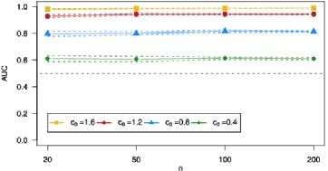
Figure 2: AUC scores in simulation study with $\mu_{j}=c_{0}(20/n)^{1/2}$, in the example of Section 5.1.

We also explored cases where the nonzero $\mu_{j}$’s took random values, in particular where they were drawn randomly and uniformly from the interval $[0,c_{0}(20/n)^{1/2}]$. This case is more challenging, since the genuine signals are now strictly smaller than in the previous situation. Therefore, it comes as no surprise to learn that the $\mathrm{AUC}$ levels for each $c_{0}$ are reduced. However, the overall pattern of stability with respect to $n$ is still evident, with very slightly more variation than in the case of fixed $\mu_{j}$’s.

5.2 Influence of dependence on misranking performance

Next, we discuss the effects of dependent noise $Z_{ij}$ in the model at (4). We take the noise to be a moving average of order 1, that is, $Z_{ij}=\rho Z_{i,j-1}+(1-\rho^{2})^{1/2}\varepsilon_{i,j}$, where the $\varepsilon_{i,j}$’s are independent and normal N$(0,1)$. Thus, $Z_{ij}$ and $Z_{ik}$ are correlated for all pairs $(j,k)$, with the coefficient of correlation decaying exponentially fast in $|j-k|$. The value of $c_{0}$ is fixed at 1.2, and nonzero $\mu_{j}$’s are chosen uniformly in $[0,c_{0}(20/n)^{1/2}]$. The values of $n$, $p$ and the number of true signals are as in Section 5.1.

Table 1 gives values of Monte Carlo approximations to the means and standard deviations of $\mathrm{AUC}$ scores when the features for which $\mu_{j}$ is nonzero are grouped together among the lowest values of $j$, as in the discussion following Theorem 4. The main observation is that while mean $\mathrm{AUC}$ remains stable across the table, the variability of $\mathrm{AUC}$ is much greater when strong dependence exists. For instance, if $n=200$ then when $\rho=0.99$ the standard deviation of $\mathrm{AUC}$ scores is ten times larger than when $\rho=0$. The presence of dependence makes the problem significantly more difficult; it effectively inserts an element of randomness into the process of correctly ranking important features.

Table 2 shows results in the same setting, except that the indices of features where $\mu_{j}$ is nonzero are distributed randomly between 1 and $p$. There is again a high degree of stability, but variability is comparatively less than that in Table 1, consistent with the discussion in Section 3.3. In particular, by randomly distributing the indices of the nonzero $\mu_{j}$’s we effectively reduce dependence among the features that are important, and so, reflecting the results in Table 1, the problem becomes less statistically challenging.

Table 1: Mean and standard deviation of $\mathrm{AUC}$ scores for simulation with correlated noise and grouped effects

	AUC means				AUC std dev.
$\rho$	$n=20$	$n=50$	$n=100$	$n=200$	$n=20$	$n=50$	$n=100$	$n=200$
$-0.99$	0.725	0.698	0.706	0.709	0.136	0.078	0.039	0.018
$-0.75$	0.704	0.717	0.715	0.712	0.064	0.022	0.012	0.006
$-0.50$	0.650	0.705	0.718	0.711	0.070	0.024	0.011	0.006
$-0.25$	0.702	0.725	0.706	0.716	0.062	0.025	0.012	0.007
0.00	0.699	0.707	0.711	0.714	0.070	0.027	0.012	0.006
0.25	0.687	0.714	0.707	0.712	0.080	0.032	0.015	0.007
0.50	0.666	0.682	0.713	0.713	0.094	0.037	0.017	0.009
0.75	0.715	0.710	0.718	0.719	0.101	0.047	0.025	0.013
0.99	0.662	0.725	0.708	0.704	0.259	0.157	0.107	0.065

Table 2: Mean and standard deviation of $\mathrm{AUC}$ scores for simulation with correlated noise and randomised effects

	AUC means				AUC std dev.
$\rho$	$n=20$	$n=50$	$n=100$	$n=200$	$n=20$	$n=50$	$n=100$	$n=200$
$-0.99$	0.712	0.712	0.713	0.715	0.139	0.058	0.032	0.016
$-0.75$	0.702	0.710	0.713	0.714	0.078	0.030	0.014	0.008
$-0.50$	0.705	0.710	0.711	0.714	0.076	0.032	0.015	0.008
$-0.25$	0.706	0.705	0.713	0.714	0.078	0.032	0.015	0.007
0.00	0.696	0.709	0.714	0.712	0.077	0.030	0.015	0.007
0.25	0.698	0.712	0.710	0.714	0.078	0.034	0.016	0.008
0.50	0.703	0.713	0.714	0.714	0.081	0.030	0.016	0.007
0.75	0.698	0.712	0.711	0.714	0.088	0.034	0.016	0.008
0.99	0.741	0.721	0.712	0.710	0.195	0.091	0.053	0.024

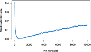
Figure 3: Ideal prediction success for the example of Section 5.3.

5.3 Prediction in a large simulated problem

Here we present the analysis of a single simulated dataset, demonstrating how our approach performs when the centroid classifier is used. We take $p=10\mbox{, }000$ and $n=100$ (50 for each class). Ten percent of the variables $X_{ij}$ (in the model at (4)) include a nonzero signal. These $\mu_{j}$’s are drawn from the uniform distribution on $[0,0.35]$, and the noise variables $Z_{ij}$ are independent $N(0,1)$. This is a particularly difficult problem, since the signals are very weak compared to the noise, and sample size is quite small.

Figure 3 shows the prediction performance of the centroid classifier on a test set of 1000 replicates in the case of “ideal feature selection,” where the 1000 features with nonzero signals are selected first, in decreasing order of signal strength, followed by the 9000 features where the signal is not present. In particular, the order is not chosen empirically. The minimum of the graph occurs at 449 features (out of a maximum of 1000), and corresponds to a misclassification rate of only 0.5%. The decrease in predictive performance caused by less useful, or redundant, features is apparent from the figure; the weaker genuine features actually hurt prediction performance because they contain more noise than signal. Also of note is the fact that a large number of features is needed to obtain good prediction. For example, if attention is confined only to the strongest 50 features then the misclassification rate increases to 16%.

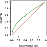
Figure 4: ROC plot for feature ranking in the example of Section 5.3.

For the same dataset, we undertook feature ranking based on the values of ${\hat{\ell}}_{j}$, defined at (3). The result was the ROC chart in Figure 4. There the value of $k$ in the ranking ${\hat{\jmath}}_{1},\ldots,{\hat{\jmath}}_{k},{\hat{\jmath}}_{k+1},\ldots,{\hat{\jmath}}_{p}$, defined in the sentence below (3), is represented as $k/p$ on the horizontal axis, and the vertical axis depicts the value of ${\hat{\ell}}_{{\hat{\jmath}}_{k}}/{\hat{\ell}}_{{\hat{\jmath}}_{1}}$, a ratio of two negative numbers. The area under the empirical curve, that is, $\mathrm{AUC}$, equals 0.626, meaning that a fraction $1-0.626\approx 37\%$ of the paired scores correspond to a misranking. The ROC curve is indexed by model size, with bottom left denoting an empty model and the top right a full model. For a given model size, we can read off the chart the corresponding sensitivity, or proportion of true important features included, and the false positive rate, or proportion of redundant features in the model. Ideally a model should have high sensitivity and low false positive rate, and the chart indicates the tradeoff between the two for various model sizes.

Figure 5 shows how prediction accuracy varies with model size. Performance is now clearly a long way from that represented in Figure 3, where the 1000 features with nonzero signals were listed first in decreasing order of strength. The minimum misclassified rate is now 13.7%, and requires the use of 3258 of the 10,000 features. As discussed in the previous paragraph, every model size corresponds to a position on the ROC plot in Figure 4, in this case $(0.31,0.51)$. Hence the optimal model found here contains 51% of the genuine features, and 31% of the redundant ones.

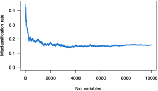
Figure 5: Performance using feature ranking and centroid classifier for the example of Section 5.3.

We next explore stage (3) of the four-stage algorithm suggested in Section 2.1, addressing in turn each of the approaches (3a)–(3c) discussed in Section 2.3. We implement the threshold method, (3a), by comparison with a randomised model where the observed classes $I_{i}$ are scrambled and likelihoods recalculated, and employ the approach suggested in the second paragraph of Section 4; see (16). In particular, the threshold is chosen by computing the $100\alpha$th percentile of scores for the scrambled data. Doing this for $\alpha=0.2$ corresponds to seeking a false positive rate of 0.2. In the numerical example that we are considering here, this recovers a model with 2159 predictors and produces a test set misclassification rate of 16.8%. A model this size corresponds to the point (0.196, 0.40) on the ROC chart. Notice that we have effectively targeted the false positive rate of $\alpha=0.2$ via this approach.

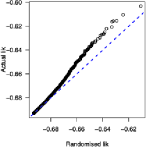
Figure 6: Comparison of actual and randomised log-likelihoods in the example of Section 5.3.

To provide an example of the change-point method, (3b), suggested in Section 2.3 for choosing model size, we consider the ratio of the sorted likelihoods from the original and scrambled rankings. These are plotted in Figure 6, along with a $45^{\circ}$ line. Starting with the weakest features, we expect the ratio to remain near 1 until a sizeable number of features that genuinely contain a positive signal cause the ratio to shrink. For this purpose we can use the simple change-point statistic for detecting a change in the mean (see Chapter 2 of Csörgő and Horváth [12]),

$$T(t)=n^{-1/2}\bigl{\{}S(nt)-tS(n)\bigr{\}},$$

where $S(k)$ equals the cumulative sum of the first $k$ ratios, and $t\in(0,1)$ denotes the examined proportion of the dataset. This leads to a model with 1760 features and a misclassification rate of 16.2%, comparable to that when using method (3a). This model size corresponds to the point (0.16, 0.36) on the ROC plot.

Finally, in reference to the classifier-based approach (3c) suggested in Section 2.3, we note that the apparent error rate can be driven quickly to zero without the actual error rate being reduced as much as it is if we employ methods (3a) or (3b). For example, when using (3c) in conjunction with the centroid classifier the “best” model, with apparent error rate equal to zero, occurs when just 39 features are selected; but the misclassification rate on the test set is 32.5%, almost twice that obtained for either of methods (3a) and (3b).

5.4 Results for microarray data examples

A challenge when using our methodology to analyse previously considered real datasets is that the latter were possibly considered because they illustrate cases where only a very small number of features determine the class label. In particular, contrary to the concerns raised by Goldstein [29], the number of influential components is quite small. To simplify matters, we demonstrate here that likelihood based ranking is a powerful tool for improving a wide variety of classifiers. We make use of three well-known sets of microarray data. These relate, respectively, to leukemia (Golub et al. [30]), colon cancer (Alon et al. [2]) and prostate cancer (Singh et al.  [39]) and have 7129, 2000 and 6033 components, respectively. Dettling [13] and Donoho and Jin [18] discuss the performance of a variety of classifiers on these datasets, using a two-thirds/one-third split of the data into training and test samples. Their results are reported in Table 3. Readers may refer to the above papers for details on specific methods.

=250pt Method Leukemia Colon Prostate Bagboo 4.08 16.10 7.53 Boost 5.67 19.14 8.71 RanFor 1.92 14.86 9.00 SVM 1.83 15.05 7.88 DLDA 2.92 12.86 14.18 KNN 3.83 16.38 10.59 PAM 3.55 13.53 8.87 HCT 2.86 13.77 9.47

Table 3: Percentage misclassification rate of different methods on microarray datasets

Table 4: Performance of best methods on reduced datasets, using likelihood based ranking

	Leukemia		Colon		Prostate
Prop.	SVM	RanFor	RDA	RanFor	PAM	RanFor
0.0025	34.72	4.58	14.29	16.58	8.82	8.00
0.005	34.61	3.78	13.00	15.71	8.37	7.67
0.01	6.86	3.36	13.13	15.77	7.84	7.73
0.025	1.89	2.97	13.10	15.74	7.16	8.20
0.05	1.67	2.58	13.26	15.16	7.29	8.55
0.10	1.58	2.50	13.19	14.94	7.02	8.90
0.15	1.67	2.22	13.16	14.94	7.10	9.14
0.25	1.64	2.36	12.90	15.03	7.06	9.49
0.375	1.61	2.11	12.87	15.52	6.82	9.67
0.50	1.58	2.22	13.00	15.58	6.82	9.90
0.75	1.53	2.36	12.97	16.13	7.02	9.80
1.00	1.61	2.31	13.00	16.32	7.04	10.24

To test the effectiveness of likelihood-based ranking, we chose the best classification method and the random forest classifier (a consistent performer) for each of the datasets. An extra step was added to each cross-validation fold; the two-thirds training data was used to rank features based on the likelihood score, and then only a proportion of the top-ranked features were used to estimate the final model. The results are presented in Table 4. The last row of the table shows results for the full dataset; they should in theory match those in Table 3, with differences attributable to tuning approaches. We could not reproduce the accuracy reported for DLDA on the colon dataset, and so used the next best method (PAM).

In each case, accuracy can be improved by reducing the model size. For the best classifiers on each dataset, this effect was small but noticeable; for the leukemia data, dimension was reduced by 25% and error by 5%; for the colon dataset, dimension was reduced by 62.5% and error by 1%; and for the prostate dataset, dimension was reduced by 62.5% and error by 3%. For the random forest models, the results were even more pronounced, with marked improvement in prediction and significant dimension reduction. For the prostate dataset, the error was reduced by 25%, using just 0.005 of the available features in each fold. This suggests that the likelihood based ranking method can effectively control the sparsity of a model and potentially improve model performance.

While firm conclusions are difficult here, we argue that this analysis presents evidence for a large number of relatively weak effects contributing to a model. Indeed, in all but one case we would prefer a model size larger than the dozens, or fewer, used in many conventional approaches to feature selection. Furthermore, our feature ranking appears to be a useful means of determining the effective model size.

5.5 Results for analysis of SNP data

We applied our methodology to SNP data collected to study multiple sclerosis (ANZgene [3]; Wade [43]). The original dataset consisted of 5031 subjects, which were collected by two organisations: the Australian and New Zealand multiple sclerosis genetic consortium (ANZgene) and the Wellcome Trust Multiple Sclerosis Genetic Consortium 2. For data permission reasons, we restrict our analysis to 3606 collected by ANZgene. This part consists of 1618 case subjects (positive response) and 1988 control subjects (zero response).

For each of the subjects, we have 300,900 corresponding SNP measurements, collected from different locations on the genome of each patient. Each of these variables takes the values 0, 1 or 2, which we treat as numeric. There were a small number of missing values, which we addressed by setting them equal to the median value for that SNP.

The dataset was randomly divided into two-thirds training data and one-third test data. Likelihood scores were calculated, and SNPs ranked, based on their improvement over AIC. We then built three sets of models:

• The centroid classifier using the top ranked $1,2,\ldots,30\mbox{,}099$ variables. Note that this means that the final model was fitted using 10% of the total variables;

• A tuned SVM classifier using the top ranked $20,40,60,\ldots,4000$ variables; and

• A random forest classifier using the top ranked $20,40,60,\ldots,4000$ variables.

The SVM and random forest models were not fitted beyond 4000 variables because these were infeasible on desktop computers. For each model, the classification error rate was measured on the test dataset. These results are presented in Figure 7.

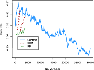
Figure 7: Comparison of error rates on the multiple sclerosis SNP data.

We make two comments regarding these results. First, the trend in the centroid classifier gives strong evidence of a large number of weak effects; the performance continues to improve as more variables are added, suggesting that there is useful information in the full top $10\%$ of the ranked variables. Second, the SVM and random forest approaches performed better using a smaller number of SNPs, but worse when compared to the large centroid models, again supporting the idea of many weak effects. We would expect that adaptations of approaches like SVM to large numbers of variables could also offer good performance.

References

- [1] {barticle}[mr] \bauthor\bsnmAbramovich, \bfnmFelix\binitsF., \bauthor\bsnmBenjamini, \bfnmYoav\binitsY., \bauthor\bsnmDonoho, \bfnmDavid L.\binitsD.L. &\bauthor\bsnmJohnstone, \bfnmIain M.\binitsI.M. (\byear2006). \btitleAdapting to unknown sparsity by controlling the false discovery rate. \bjournalAnn. Statist. \bvolume34 \bpages584–653. \biddoi=10.1214/009053606000000074, issn=0090-5364, mr=2281879 \bptokimsref \endbibitem
- [2] {barticle}[pbm] \bauthor\bsnmAlon, \bfnmU.\binitsU., \bauthor\bsnmBarkai, \bfnmN.\binitsN., \bauthor\bsnmNotterman, \bfnmD. A.\binitsD.A., \bauthor\bsnmGish, \bfnmK.\binitsK., \bauthor\bsnmYbarra, \bfnmS.\binitsS., \bauthor\bsnmMack, \bfnmD.\binitsD. &\bauthor\bsnmLevine, \bfnmA. J.\binitsA.J. (\byear1999). \btitleBroad patterns of gene expression revealed by clustering analysis of tumor and normal colon tissues probed by oligonucleotide arrays. \bjournalProc. Natl. Acad. Sci. USA \bvolume96 \bpages6745–6750. \bidissn=0027-8424, pmcid=21986, pmid=10359783 \bptokimsref \endbibitem
- [3] {bmisc}[pbm] \borganizationAustralia and New Zealand Multiple Sclerosis Genetics Consortium (ANZgene). (\byear2009). \bhowpublishedGenome-wide association study identifies new multiple sclerosis susceptibility loci on chromosomes 12 and 20. Nat. Genet. 41 824–828. \biddoi=10.1038/ng.396, issn=1546-1718, pii=ng.396, pmid=19525955 \bptokimsref \endbibitem
- [4] {barticle}[mr] \bauthor\bsnmBenjamini, \bfnmYoav\binitsY. &\bauthor\bsnmHochberg, \bfnmYosef\binitsY. (\byear1995). \btitleControlling the false discovery rate: A practical and powerful approach to multiple testing. \bjournalJ. R. Stat. Soc. Ser. B Stat. Methodol. \bvolume57 \bpages289–300. \bidissn=0035-9246, mr=1325392 \bptokimsref \endbibitem
- [5] {barticle}[mr] \bauthor\bsnmBickel, \bfnmPeter J.\binitsP.J. &\bauthor\bsnmLevina, \bfnmElizaveta\binitsE. (\byear2004). \btitleSome theory of Fisher’s linear discriminant function, ‘naive Bayes,’ and some alternatives when there are many more variables than observations. \bjournalBernoulli \bvolume10 \bpages989–1010. \biddoi=10.3150/bj/1106314847, issn=1350-7265, mr=2108040 \bptokimsref \endbibitem
- [6] {barticle}[mr] \bauthor\bsnmBreiman, \bfnmLeo\binitsL. (\byear1995). \btitleBetter subset regression using the nonnegative garrote. \bjournalTechnometrics \bvolume37 \bpages373–384. \biddoi=10.2307/1269730, issn=0040-1706, mr=1365720 \bptokimsref \endbibitem
- [7] {barticle}[mr] \bauthor\bsnmBreiman, \bfnmLeo\binitsL. (\byear1996). \btitleHeuristics of instability and stabilization in model selection. \bjournalAnn. Statist. \bvolume24 \bpages2350–2383. \biddoi=10.1214/aos/1032181158, issn=0090-5364, mr=1425957 \bptokimsref \endbibitem
- [8] {barticle}[mr] \bauthor\bsnmCandes, \bfnmEmmanuel\binitsE. &\bauthor\bsnmTao, \bfnmTerence\binitsT. (\byear2007). \btitleThe Dantzig selector: Statistical estimation when is much larger than . \bjournalAnn. Statist. \bvolume35 \bpages2313–2351. \biddoi=10.1214/009053606000001523, issn=0090-5364, mr=2382644 \bptokimsref \endbibitem
- [9] {bbook}[mr] \beditor\bsnmCarlstein, \bfnmEdward\binitsE., \beditor\bsnmMüller, \bfnmHans-Georg\binitsH.G. &\beditor\bsnmSiegmund, \bfnmDavid\binitsD., eds. (\byear1994). \btitleChange-Point Problems. \bseriesInstitute of Mathematical Statistics Lecture Notes—Monograph Series \bvolume23. \blocationHayward, CA: \bpublisherIMS. \bidmr=1477909 \bptokimsref \endbibitem
- [10] {barticle}[author] \bauthor\bsnmChen, \bfnmS. S.\binitsS.S., \bauthor\bsnmDonoho, \bfnmD. L.\binitsD.L. &\bauthor\bsnmSaunders, \bfnmM. A.\binitsM.A. (\byear1998). \btitleAtomic decomposition by basis pursuit. \bjournalSIAM J. Sci. Comp. \bvolume20 \bpages33–61. \bptokimsref \endbibitem
- [11] {bbook}[mr] \bauthor\bsnmChen, \bfnmJie\binitsJ. &\bauthor\bsnmGupta, \bfnmA. K.\binitsA.K. (\byear2000). \btitleParametric Statistical Change Point Analysis. \blocationBoston, MA: \bpublisherBirkhäuser. \bidmr=1761850 \bptokimsref \endbibitem
- [12] {bbook}[mr] \bauthor\bsnmCsörgő, \bfnmMiklós\binitsM. &\bauthor\bsnmHorváth, \bfnmLajos\binitsL. (\byear1997). \btitleLimit Theorems in Change-Point Analysis. \bseriesWiley Series in Probability and Statistics. \blocationChichester: \bpublisherWiley. \bidmr=2743035 \bptokimsref \endbibitem
- [13] {barticle}[pbm] \bauthor\bsnmDettling, \bfnmMarcel\binitsM. (\byear2004). \btitleBagBoosting for tumor classification with gene expression data. \bjournalBioinformatics \bvolume20 \bpages3583–3593. \biddoi=10.1093/bioinformatics/bth447, issn=1367-4803, pii=bth447, pmid=15466910 \bptokimsref \endbibitem
- [14] {barticle}[mr] \bauthor\bsnmDonoho, \bfnmDavid L.\binitsD.L. (\byear2006). \btitleFor most large underdetermined systems of linear equations the minimal -norm solution is also the sparsest solution. \bjournalComm. Pure Appl. Math. \bvolume59 \bpages797–829. \biddoi=10.1002/cpa.20132, issn=0010-3640, mr=2217606 \bptokimsref \endbibitem
- [15] {barticle}[mr] \bauthor\bsnmDonoho, \bfnmDavid L.\binitsD.L. (\byear2006). \btitleFor most large underdetermined systems of equations, the minimal -norm near-solution approximates the sparsest near-solution. \bjournalComm. Pure Appl. Math. \bvolume59 \bpages907–934. \biddoi=10.1002/cpa.20131, issn=0010-3640, mr=2222440 \bptokimsref \endbibitem
- [16] {barticle}[mr] \bauthor\bsnmDonoho, \bfnmDavid L.\binitsD.L. &\bauthor\bsnmElad, \bfnmMichael\binitsM. (\byear2003). \btitleOptimally sparse representation in general (nonorthogonal) dictionaries via minimization. \bjournalProc. Natl. Acad. Sci. USA \bvolume100 \bpages2197–2202 (electronic). \biddoi=10.1073/pnas.0437847100, issn=1091-6490, mr=1963681 \bptokimsref \endbibitem
- [17] {barticle}[mr] \bauthor\bsnmDonoho, \bfnmDavid L.\binitsD.L. &\bauthor\bsnmHuo, \bfnmXiaoming\binitsX. (\byear2001). \btitleUncertainty principles and ideal atomic decomposition. \bjournalIEEE Trans. Inform. Theory \bvolume47 \bpages2845–2862. \biddoi=10.1109/18.959265, issn=0018-9448, mr=1872845 \bptokimsref \endbibitem
- [18] {barticle}[auto:STB—2013/06/05—13:45:01] \bauthor\bsnmDonoho, \bfnmD. L.\binitsD.L. &\bauthor\bsnmJin, \bfnmJ.\binitsJ. (\byear2008). \btitleHigher criticism thresholding: Optimal feature selection when useful features and rare and weak. \bjournalProc. Natl. Acad. Sci. USA \bvolume105 \bpages14790–14795. \bptokimsref \endbibitem
- [19] {barticle}[mr] \bauthor\bsnmDonoho, \bfnmDavid\binitsD. &\bauthor\bsnmJin, \bfnmJiashun\binitsJ. (\byear2009). \btitleFeature selection by higher criticism thresholding achieves the optimal phase diagram. \bjournalPhilos. Trans. R. Soc. Lond. Ser. A Math. Phys. Eng. Sci. \bvolume367 \bpages4449–4470. \biddoi=10.1098/rsta.2009.0129, issn=1364-503X, mr=2546396 \bptokimsref \endbibitem
- [20] {bbook}[mr] \bauthor\bsnmDuda, \bfnmRichard O.\binitsR.O., \bauthor\bsnmHart, \bfnmPeter E.\binitsP.E. &\bauthor\bsnmStork, \bfnmDavid G.\binitsD.G. (\byear2001). \btitlePattern Classification, \bedition2nd ed. \blocationNew York: \bpublisherWiley-Interscience. \bidmr=1802993 \bptokimsref \endbibitem
- [21] {barticle}[mr] \bauthor\bsnmFan, \bfnmJianqing\binitsJ. &\bauthor\bsnmFan, \bfnmYingying\binitsY. (\byear2008). \btitleHigh-dimensional classification using features annealed independence rules. \bjournalAnn. Statist. \bvolume36 \bpages2605–2637. \biddoi=10.1214/07-AOS504, issn=0090-5364, mr=2485009 \bptokimsref \endbibitem
- [22] {barticle}[mr] \bauthor\bsnmFan, \bfnmJianqing\binitsJ. &\bauthor\bsnmLi, \bfnmRunze\binitsR. (\byear2001). \btitleVariable selection via nonconcave penalized likelihood and its oracle properties. \bjournalJ. Amer. Statist. Assoc. \bvolume96 \bpages1348–1360. \biddoi=10.1198/016214501753382273, issn=0162-1459, mr=1946581 \bptokimsref \endbibitem
- [23] {bincollection}[mr] \bauthor\bsnmFan, \bfnmJianqing\binitsJ. &\bauthor\bsnmLi, \bfnmRunze\binitsR. (\byear2006). \btitleStatistical challenges with high dimensionality: Feature selection in knowledge discovery. In \bbooktitleInternational Congress of Mathematicians. Vol. III (\beditor\bfnmM.\binitsM. \bsnmSanz-Sole, \beditor\bfnmJ.\binitsJ. \bsnmSoria, \beditor\bfnmJ. L.\binitsJ.L. \bsnmVarona &\beditor\bfnmJ.\binitsJ. \bsnmVerdera, eds.) \bpages595–622. \blocationZürich: \bpublisherEur. Math. Soc. \bidmr=2275698 \bptokimsref \endbibitem
- [24] {barticle}[auto:STB—2013/06/05—13:45:01] \bauthor\bsnmFan, \bfnmJ.\binitsJ. &\bauthor\bsnmLv, \bfnmJ.\binitsJ. (\byear2008). \btitleSure independence screening for ultra-high dimensional feature space. \bjournalJ. R. Stat. Soc. Ser. B Stat. Methodol. \bvolume70 \bpages849–911. \bptokimsref \endbibitem
- [25] {barticle}[pbm] \bauthor\bsnmFan, \bfnmJianqing\binitsJ. &\bauthor\bsnmRen, \bfnmYi\binitsY. (\byear2006). \btitleStatistical analysis of DNA microarray data in cancer research. \bjournalClin. Cancer Res. \bvolume12 \bpages4469–4473. \biddoi=10.1158/1078-0432.CCR-06-1033, issn=1078-0432, pii=12/15/4469, pmid=16899590 \bptokimsref \endbibitem
- [26] {barticle}[mr] \bauthor\bsnmFan, \bfnmJianqing\binitsJ. &\bauthor\bsnmSong, \bfnmRui\binitsR. (\byear2010). \btitleSure independence screening in generalized linear models with NP-dimensionality. \bjournalAnn. Statist. \bvolume38 \bpages3567–3604. \biddoi=10.1214/10-AOS798, issn=0090-5364, mr=2766861 \bptokimsref \endbibitem
- [27] {barticle}[mr] \bauthor\bsnmGao, \bfnmHong-Ye\binitsH.Y. (\byear1998). \btitleWavelet shrinkage denoising using the non-negative garrote. \bjournalJ. Comput. Graph. Statist. \bvolume7 \bpages469–488. \biddoi=10.2307/1390677, issn=1061-8600, mr=1665666 \bptokimsref \endbibitem
- [28] {barticle}[mr] \bauthor\bsnmGenovese, \bfnmChristopher R.\binitsC.R., \bauthor\bsnmJin, \bfnmJiashun\binitsJ., \bauthor\bsnmWasserman, \bfnmLarry\binitsL. &\bauthor\bsnmYao, \bfnmZhigang\binitsZ. (\byear2012). \btitleA comparison of the lasso and marginal regression. \bjournalJ. Mach. Learn. Res. \bvolume13 \bpages2107–2143. \bidissn=1532-4435, mr=2956354 \bptokimsref \endbibitem
- [29] {barticle}[auto:STB—2013/06/05—13:45:01] \bauthor\bsnmGoldstein, \bfnmD. B.\binitsD.B. (\byear2009). \btitleCommon genetic variation and human traits. \bjournalNew England J. Med. \bvolume360 \bpages1696–1698. \bptokimsref \endbibitem
- [30] {barticle}[pbm] \bauthor\bsnmGolub, \bfnmT. R.\binitsT.R., \bauthor\bsnmSlonim, \bfnmD. K.\binitsD.K., \bauthor\bsnmTamayo, \bfnmP.\binitsP., \bauthor\bsnmHuard, \bfnmC.\binitsC., \bauthor\bsnmGaasenbeek, \bfnmM.\binitsM., \bauthor\bsnmMesirov, \bfnmJ. P.\binitsJ.P., \bauthor\bsnmColler, \bfnmH.\binitsH., \bauthor\bsnmLoh, \bfnmM. L.\binitsM.L., \bauthor\bsnmDowning, \bfnmJ. R.\binitsJ.R., \bauthor\bsnmCaligiuri, \bfnmM. A.\binitsM.A., \bauthor\bsnmBloomfield, \bfnmC. D.\binitsC.D. &\bauthor\bsnmLander, \bfnmE. S.\binitsE.S. (\byear1999). \btitleMolecular classification of cancer: Class discovery and class prediction by gene expression monitoring. \bjournalScience \bvolume286 \bpages531–537. \bidissn=0036-8075, pii=7911, pmid=10521349 \bptokimsref \endbibitem
- [31] {barticle}[mr] \bauthor\bsnmHall, \bfnmPeter\binitsP. &\bauthor\bsnmMiller, \bfnmHugh\binitsH. (\byear2009). \btitleUsing generalized correlation to effect variable selection in very high dimensional problems. \bjournalJ. Comput. Graph. Statist. \bvolume18 \bpages533–550. \biddoi=10.1198/jcgs.2009.08041, issn=1061-8600, mr=2751640 \bptokimsref \endbibitem
- [32] {barticle}[mr] \bauthor\bsnmHall, \bfnmPeter\binitsP. &\bauthor\bsnmWang, \bfnmQiying\binitsQ. (\byear2010). \btitleStrong approximations of level exceedences related to multiple hypothesis testing. \bjournalBernoulli \bvolume16 \bpages418–434. \biddoi=10.3150/09-BEJ220, issn=1350-7265, mr=2668908 \bptokimsref \endbibitem
- [33] {barticle}[auto:STB—2013/06/05—13:45:01] \bauthor\bsnmHanley, \bfnmJ. A.\binitsJ.A. &\bauthor\bsnmMcneil, \bfnmB. J.\binitsB.J. (\byear1982). \btitleThe meaning and use of the area under a receiver operating characteristic (ROC) curve. \bjournalRadiology \bvolume143 \bpages29–36. \bptokimsref \endbibitem
- [34] {bbook}[mr] \bauthor\bsnmHastie, \bfnmTrevor\binitsT., \bauthor\bsnmTibshirani, \bfnmRobert\binitsR. &\bauthor\bsnmFriedman, \bfnmJerome\binitsJ. (\byear2001). \btitleThe Elements of Statistical Learning: Data Mining, Inference, and Prediction. \bseriesSpringer Series in Statistics. \blocationNew York: \bpublisherSpringer. \bidmr=1851606 \bptokimsref \endbibitem
- [35] {barticle}[auto:STB—2013/06/05—13:45:01] \bauthor\bsnmHirschhorn, \bfnmJ. N.\binitsJ.N. (\byear2009). \btitleGenomewide association studies—Illuminating biologic pathways. \bjournalNew England J. Med. \bvolume360 \bpages1699–1701. \bptokimsref \endbibitem
- [36] {barticle}[mr] \bauthor\bsnmJin, \bfnmJiashun\binitsJ. (\byear2009). \btitleImpossibility of successful classification when useful features are rare and weak. \bjournalProc. Natl. Acad. Sci. USA \bvolume106 \bpages8859–8864. \biddoi=10.1073/pnas.0903931106, issn=1091-6490, mr=2520682 \bptokimsref \endbibitem
- [37] {barticle}[auto:STB—2013/06/05—13:45:01] \bauthor\bsnmKraft, \bfnmP.\binitsP. &\bauthor\bsnmHunter, \bfnmD. J.\binitsD.J. (\byear2009). \btitleGenetic risk prediction—Are we there yet? \bjournalNew England J. Med. \bvolume360 \bpages1701–1703. \bptokimsref \endbibitem
- [38] {bbook}[auto:STB—2013/06/05—13:45:01] \bauthor\bsnmShakhnarovich, \bfnmG.\binitsG., \bauthor\bsnmDarrell, \bfnmT.\binitsT. &\bauthor\bsnmIndyk, \bfnmP.\binitsP. (\byear2005). \btitleNearest-Neighbor Methods in Learning and Vision. Theory and Practice. \blocationCambridge, MA: \bpublisherMIT Press. \bptokimsref \endbibitem
- [39] {barticle}[auto:STB—2013/06/05—13:45:01] \bauthor\bsnmSingh, \bfnmD.\binitsD., \bauthor\bsnmFebbo, \bfnmP. G.\binitsP.G., \bauthor\bsnmRoss, \bfnmK.\binitsK., \bauthor\bsnmJackson, \bfnmD. G.\binitsD.G., \bauthor\bsnmManola, \bfnmJ.\binitsJ., \bauthor\bsnmLadd, \bfnmC.\binitsC., \bauthor\bsnmTamayo, \bfnmP.\binitsP., \bauthor\bsnmRenshaw, \bfnmA. A. D.\binitsA.A.D., \bauthor\bsnmAmico, \bfnmA. V.\binitsA.V. &\bauthor\bsnmRichie, \bfnmJ. P.\binitsJ.P. (\byear2002). \btitleGene expression correlates of clinical prostate cancer behavior. \bjournalCancer Cell \bvolume1 \bpages203–09. \bptokimsref \endbibitem
- [40] {barticle}[mr] \bauthor\bsnmTibshirani, \bfnmRobert\binitsR. (\byear1996). \btitleRegression shrinkage and selection via the lasso. \bjournalJ. R. Stat. Soc. Ser. B Stat. Methodol. \bvolume58 \bpages267–288. \bidissn=0035-9246, mr=1379242 \bptokimsref \endbibitem
- [41] {barticle}[auto:STB—2013/06/05—13:45:01] \bauthor\bsnmTibshirani, \bfnmR.\binitsR., \bauthor\bsnmHastie, \bfnmT.\binitsT., \bauthor\bsnmNarasimhan, \bfnmB.\binitsB. &\bauthor\bsnmChu, \bfnmG.\binitsG. (\byear2002). \btitleDiagnosis of multiple cancer types by shrunken centroids of gene expression. \bjournalProc. Natl. Acad. Sci. USA \bvolume99 \bpages6567–572. \bptokimsref \endbibitem
- [42] {barticle}[mr] \bauthor\bsnmTropp, \bfnmJoel A.\binitsJ.A. (\byear2005). \btitleRecovery of short, complex linear combinations via minimization. \bjournalIEEE Trans. Inform. Theory \bvolume51 \bpages1568–1570. \biddoi=10.1109/TIT.2005.844057, issn=0018-9448, mr=2241515 \bptokimsref \endbibitem
- [43] {bmisc}[auto:STB—2013/06/05—13:45:01] \bauthor\bsnmWade, \bfnmN.\binitsN. (\byear2009). \bhowpublishedGenes show limited value in predicting diseases. New York Times, April 15. Available at www.nytimes.com/2009/04/16/health/research/16gene.html. \bptokimsref \endbibitem
- [44] {bbook}[mr] \bauthor\bsnmWu, \bfnmYanhong\binitsY. (\byear2005). \btitleInference for Change-Point and Post-Change Means After a CUSUM Test. \bseriesLecture Notes in Statistics \bvolume180. \blocationNew York: \bpublisherSpringer. \bidmr=2142337 \bptokimsref \endbibitem