Abstract

Models based on Universal Extra Dimensions predict Kaluza-Klein (KK) excitations of all Standard Model (SM) particles. We examine the pair production of KK excitations of top- and bottom-quarks at the Large Hadron Collider. Once produced, the KK top/bottom quarks can decay to $b$-quarks, leptons and the lightest KK-particle, $\gamma_{1}$, resulting in 2 $b$-jets, two opposite sign leptons and missing transverse momentum, thereby mimicing top-pair production. We show that, with a proper choice of kinematic cuts, an integrated luminosity of 100 fb^-1 would allow a discovery for an inverse radius upto $R^{-1}=750$ GeV.

Key Words:  Universal Extra Dimension, LHC, etc.

I Introduction

The twin primary goals of Large Hadron Collider (LHC), expected to start operating by the end of 2009 are to understand the mechanism for electro-weak symmetry breaking (EWSB) as well as uncover any new dynamics that may be operative at the scale of a few TeVs. Two classes of theories command special attention at future experiments like the LHC: supersymmetric theories on the one hand and those invoking one or more extra space-like dimensions on the other. It should be noted that these two ideas (supersymmetry and additional dimensions) are by no means mutually exclusive.

Extra-dimensional theories can be subdivided into two main classes. The first corresponds to those wherein the Standard Model (SM) fields are confined to a (3 + 1) dimensional subspace of the full manifold. We shall not concern ourselves with such models. The second class comprises models wherein some or all of the SM fields can access the extended space-time manifold [1], whether fully or partially. Such TeV scale extra-dimensional scenarios could lead to a new mechanism of supersymmetry breaking [2], relax the upper limit of the lightest supersymmetric neutral Higgs [3], address the issue of fermion mass hierarchy from a different perspective [4], provide a cosmologically viable dark matter candidate [5], interprete the Higgs as a quark composite leading to a successful EWSB without the necessity of a fundamental scalar or Yukawa interactions [6], and lower the unification scale down to a few TeVs [7, 8, 9]. Our concern here is a specific and particularly interesting framework, called the Universal Extra Dimension (UED) scenario, characterized by a single flat extra dimension, compactified on an $S^{1}/Z_{2}$ orbifold, which is accessed by all the SM particles [1]. From a 4-dimensional viewpoint, every field will then have an infinite tower of Kaluza-Klein (KK) modes, the zero modes being identified as the corresponding SM states.

The key feature of the UED Lagrangian is that the momentum in the universal fifth direction is conserved. From a 4-dimensional perspective, this implies KK number conservation. However, boundary conditions break this symmetry, leaving behind only a conserved KK parity, defined as $(-1)^{n}$, where $n$ is the KK number. This discrete symmetry ensures that the lightest KK particle is stable (hence being a natural candidate for the Dark Matter particle [5]) and that the level-one KK-modes would be produced only in pairs. This also ensures that the KK modes do not affect electroweak processes at the tree level. And while they do contribute to higher order electroweak processes, in a loop they appear only in pairs resulting in a substantial suppression of such contributions, thereby allowing for relatively smaller KK-spacings. In spite of the infinite multiplicity of the KK states, the KK parity ensures that all electroweak observables are finite (up to one-loop)[10], and a comparison of the observable predictions with experimental data yields bounds on the compactification radius $R$. Constraints on the UED scenario from the measurement of the anomalous magnetic moment of the muon [11], flavour changing neutral currents [12, 13, 14], $Z\to b\bar{b}$ decay [15], the $\rho$ parameter [1, 16], several other electroweak precision tests [17], all conclude that $R^{-1}~{}\raisebox{-1.72218pt}{\hbox to0.0pt{$\sim$\hss}}\raisebox{1.72218pt}{$>$}~{}300$ GeV.

The fact that such a small value for $R^{-1}$ (equivalently, small KK spacings) is still allowed, renders collider search prospects very interesting both in the context of hadronic [18] and leptonic [19] colliders.

In this work, we study a very specific signal of the universal extra dimension at the Large Hadron Collider, culminating in a final state that would be very well-studied at the LHC irrespective of the existence of any such models. To be precise, we consider the pair production of the first KK-top and KK-bottom quarks at the LHC. While decaying, these may go into a pair of $b$-jets accompanied by a pair of opposite-signed leptons as well as missing transverse momentum ($p_{T}/\hskip 4.30554pt$). This specific final state also arises from the pair production and decay of top quarks and indeed forms a bedrock of top-quark study. Thus, the same data sample can be utilised for exploring the signals of UED.

The rest of paper is organised as follows. In the next section, we briefly discuss the universal extra-dimensional scenario with emphasis on its mass spectrum. In the subsequent section, we will discuss the production and decay of the first KK-top and KK-bottom quarks. We also compare the decay signal with that of SM top quarks, which will be produced copiously at the LHC. We will discuss the kinematic cuts which can seperate the UED signal from that of SM top quarks. Finally, we summarise in section IV.

II Universal Extra Dimension

The extra dimension is compactified on a circle of radius $R$ with a $Z_{2}$ orbifolding defined by identifying $y\to-y$, where $y$ denotes the fifth (compactified) coordinate. The orbifolding is crucial in generating chiral zero modes for fermions. Each component of a 5-dimensional field must be either even or odd under the orbifold projection. After integrating out the compactified dimension, the effective 4-dimensional Lagrangian can be written in terms of the respective zero modes and the KK excitations. It is instructive to take a glance at the KK mode expansions of these fields. Defining

$${\cal C}_{n}\equiv\sqrt{\frac{2}{\pi\,R}}\,\cos\,\frac{n\,y}{R}\qquad{\rm and}\qquad{\cal S}_{n}\equiv\sqrt{\frac{2}{\pi\,R}}\,\sin\,\frac{n\,y}{R}\ ,$$ (1)

the KK expansions are given by

$$\begin{array}[]{rcl}A_{\mu}(x,y)&=&\displaystyle\frac{1}{\sqrt{2}}\,A_{\mu}^{(0)}(x)\,{\cal C}_{0}+\sum^{\infty}_{n=1}A_{\mu}^{(n)}(x)\,{\cal C}_{n}\ ,\\[4.30554pt] A_{5}(x,y)&=&\displaystyle\sum^{\infty}_{n=1}A_{5}^{(n)}(x)\,{\cal S}_{n}\ ,\\[4.30554pt] \phi(x,y)&=&\displaystyle\frac{1}{\sqrt{2}}\,\phi^{(0)}(x){\cal C}_{0}+\sum^{\infty}_{n=1}\phi^{(n)}(x)\,{\cal C}_{n}\ ,\\[10.76385pt] \mathcal{Q}_{i}(x,y)&=&\displaystyle\frac{1}{\sqrt{2}}\,\mathcal{Q}_{i}(x)\,{\cal C}_{0}+\sum^{\infty}_{n=1}\left[\mathcal{Q}^{(n)}_{iL}(x)\,{\cal C}_{n}+\mathcal{Q}^{(n)}_{iR}(x)\,{\cal S}_{n}\right]\ ,\\[10.76385pt] \mathcal{U}_{i}(x,y)&=&\displaystyle\frac{1}{\sqrt{2}}\,\mathcal{U}_{i}(x)\,{\cal C}_{0}+\sum^{\infty}_{n=1}\left[\mathcal{U}^{(n)}_{iR}(x)\,{\cal C}_{n}+\mathcal{U}^{(n)}_{iL}(x)\,{\cal S}_{n}\right]\ ,\\[10.76385pt] \mathcal{D}_{i}(x,y)&=&\displaystyle\frac{1}{\sqrt{2}}\,\mathcal{D}_{i}(x)\,{\cal C}_{0}+\sum^{\infty}_{n=1}\left[\mathcal{D}^{(n)}_{iR}(x)\,{\cal C}_{n}+\mathcal{D}^{(n)}_{iL}(x)\,{\cal S}_{n}\right]\ ,\end{array}$$ (2)

where $i=1\dots 3$ denotes generations and the fields $\mathcal{Q}_{i}$, $\mathcal{U}_{i}$, and $\mathcal{D}_{i}$ describe the 5-dimensional quark weak-doublet and singlet states respectively. The zero modes thereof are identified with the 4-dimensional chiral SM quark states. The complex scalar field $\phi(x,y)$ and the gauge boson $A_{\mu}(x,y)$ are $Z_{2}$ even fields with their zero modes identified with the SM scalar doublet and SM gauge bosons respectively. On the contrary, the field $A_{5}(x,y)$, which is a real scalar transforming in the adjoint representation of the gauge group, does not have any zero mode. The KK expansions of the lepton fields are analogous to those for the quarks and are not shown for the sake of brevity.

II.1 Radiative corrections to the KK-masses

As is well known, the tree-level mass of a level-$n$ KK component is given by

$$m_{n}^{2}=m_{0}^{2}+\frac{n^{2}}{R^{2}}\ ,$$ (3)

$m_{0}$ is the mass associated with the corresponding SM field. Now, as a zeroth approximation, one may treat all the SM particles, apart from the top quark, the weak gauge bosons and the Higgs boson, to be nearly massless. This implies, that, at each KK-level, the different states are approximately degenerate. An immediate consequence would be the quasi-stability of many of the KK-fields, leading to possibly spectacular signatures in a collider environment. This, however, is only the leading order approximation and quantum corrections lift this degeneracy. Apart from the usual radiative corrections that we expect in a Minkowski-space field theory, there are additional corrections accruing from the fact of the fifth direction being a compact one. We briefly review these next.

• Bulk corrections:
  These arise due to the winding of the internal loop (lines) around the compactified direction[20], and are nonzero (and finite) only for the gauge boson KK-excitations. For the first level KK-modes, the bulk corrections are given by

  $$\begin{array}[]{rcl}\delta\,(m_{B^{n}}^{2})&=&\displaystyle-\frac{39\,\zeta(3)\,a_{1}}{2\,\pi^{2}\,R^{2}}\ ,\\[8.61108pt] \delta\,(m_{W^{n}}^{2})&=&\displaystyle-\frac{5\,\zeta(3)\,a_{2}}{2\,\pi^{2}\,R^{2}}\ ,\\[8.61108pt] \delta\,(m_{g^{n}}^{2})&=&\displaystyle-\frac{3\,\zeta(3)\,a_{3}}{2\,\pi^{2}\,R^{2}}\ ,\end{array}$$ (4)

  where $a_{i}\equiv g_{i}^{2}/16\,\pi^{2}\ ,i=1\dots 3$ with $g_{i}$ denoting the respective gauge coupling constants. The vanishing of these corrections in the limit $R\rightarrow\infty$ reflects the removal of the compactness of the fifth direction and hence the restoration of full five-dimensional Lorentz invariance.

• Orbifold corrections:
  The very process of orbifolding introduces a set of special (fixed) points in the fifth direction (two in the case of $S^{1}/Z_{2}$ compactification). This clearly violates the five-dimensional Lorentz invariance of the tree level Lagrangian. Unlike the bulk corrections, the boundary corrections are not finite, but are logarithmically divergent[20]. They are just the counterterms of the total orbifold correction, with the finite parts being completely unknown, dependent as they are on the details of the ultraviolet completion. Assuming that the boundary kinetic terms vanish at the cutoff scale $\Lambda$ ($=20$ TeV here) the corrections from the boundary terms, at a renormalization scale $\mu$ would obviously be proportional to $L_{0}\equiv\ln(\Lambda^{2}/\mu^{2})$. Denoting $m_{n}({\cal A})$ to be the tree-level mass of the $n$-th KK-component of a SM field ${\cal A}$, we have[20]

  $$\begin{array}[]{rcl}\bar{\delta}\,m_{Q^{n}}&=&\displaystyle m_{n}\,\left(3\,a_{3}+\frac{27}{16}\,a_{2}+\frac{a_{1}}{16}\right)\,L_{0}\ ,\\[8.61108pt] \bar{\delta}\,m_{u^{n}}&=&m_{n}\,\left(3\,a_{3}+a_{1}\right)\,L_{0}\ ,\\[8.61108pt] \bar{\delta}\,m_{d^{n}}&=&\displaystyle m_{n}\,\left(3\,a_{3}+\frac{a_{1}}{4}\right)\,L_{0}\ ,\\[8.61108pt] \bar{\delta}\,m_{L^{n}}&=&\displaystyle m_{n}\,\left(\frac{27}{16}\,a_{2}+\frac{9}{16}\,a_{1}\right)\,L_{0}\ ,\\[8.61108pt] \bar{\delta}\,m_{e^{n}}&=&\displaystyle\frac{9\,a_{1}}{4}\,m_{n}\,L_{0}\ ,\\[8.61108pt] \bar{\delta}\,(m_{B^{n}}^{2})&=&\displaystyle\frac{-a_{1}}{6}\,m_{n}^{2}\,L_{0}\\[8.61108pt] \bar{\delta}\,(m_{W^{n}}^{2})&=&\displaystyle\frac{15\,a_{2}}{2}\,m_{n}^{2}\,L_{0}\ ,\\[8.61108pt] \bar{\delta}\,(m_{g^{n}}^{2})&=&\displaystyle\frac{23\,a_{3}}{2}\,m_{n}^{2}\,L_{0}\ ,\\[8.61108pt] \bar{\delta}\,(m_{H^{n}}^{2})&=&\displaystyle m_{n}^{2}\,\left(\frac{3}{2}\,a_{2}+\frac{3}{4}\,a_{1}-\frac{\lambda_{H}}{16\pi^{2}}\right)L_{0}+\overline{m}_{H}^{2}\ ,\end{array}$$ (5)

  where the boundary term for the Higgs scalar, namely $\overline{m}_{H}^{2}$, is taken to be vanishing.

The KK-excitations of the neutral electroweak gauge bosons mix in a fashion analogous to their SM counterparts and the mass eigenstates and eigenvalues of the KK ‘photons’ and ‘$Z$’ bosons are obtained by diagonalizing the corresponding mass squared matrices. In the $(B_{n},W^{3}_{n})$ basis, the latter reads

$$\left(\begin{array}[]{cc}\displaystyle\frac{n^{2}}{R^{2}}+\hat{\delta}m_{B^{n}}^{2}+\frac{1}{4}g_{1}^{2}v^{2}&\displaystyle\frac{1}{4}g_{1}g_{2}v^{2}\\[8.61108pt] \displaystyle\frac{1}{4}g_{1}g_{2}v^{2}&\displaystyle\frac{n^{2}}{R^{2}}+\hat{\delta}m_{W^{n}}^{2}+\frac{1}{4}g_{2}^{2}v^{2}\end{array}\right),$$

where $\hat{\delta}$ represents the total one-loop correction, including both bulk and boundary contributions. Note that, with $v$ being just the scale of EWSB, the extent of mixing is miniscule even at $R^{-1}=500$ GeV and is progressively smaller for the higher KK-modes. As a consequence, unless $R^{-1}$ is very small, the $Z^{1}$ and $\gamma^{1}$ are, for all practical purposes, essentially $W^{1}_{3}$ and $B^{1}$. This has profound consequences in the decays of the KK-excitations.

With the mass corrections for $B^{n}$ always being negative, and the contribution from EWSB being relatively small, it is understandable that the KK-photons have masses very close to $n/R$. A further consequence is that the lightest KK-particle (LKP), and hence the Dark Matter candidate, is almost always the $\gamma^{1}$. Furthermore, of the other KK-excitations, the leptonic fields are the lightest (and nearly degenerate) followed by the weak gauge boson excitations. The quark and gluon excitations are the heaviest within a given KK-level on account of the substantial corrections due to the strong interactions.

In a similar vein, the quark excitations mix too. With the 5-dimensional theory necessarily being a non-chiral one, for every SM fermion state, there correspond two states at each KK-level (see eqn.2). These obviously mix with each other with a strength determined by the SM Yukawa coupling. Thus, while the two top-states at level one (hereafter denoted as $t^{1}_{1}$ and $t^{1}_{2}$) are split slightly, the other KK fermions are almost degenerate. This is depicted in Table 1 which lists the masses of the first KK-modes of various SM particles, after the inclusion of radiative corrections, for three representative valuesof $1/R$, namely, 300, 500 and 800 GeV.

$R^{-1}$	$m_{t^{1}_{1}}$	$m_{t^{1}_{2}}$	$m_{b^{1}_{1}},m_{b^{1}_{2}}$	$m_{L^{1}}$	$m_{e^{1}}$	$m_{g^{1}}$	$m_{{W^{\pm}}^{1}}$	$m_{Z^{1}}$	$m_{\gamma^{1}}$
300	389.0	373.5	347.6	309.0	303.3	384.3	327.4	328.6	301.5
500	599.9	587.3	585.5	515	505.5	642.3	536	542.1	501.0
800	941.6	900.3	924.9	815.9	808.7	1024.7	850.4	850.5	800.0

Table 1: One-loop corrected masses (in GeVs) for the first KK-mode of different fermions and gauge bosons for three values of the compactification radius $R$.

III Production and decay of the first level KK-top and bottom quarks

The KK-quarks being strongly interacting, their pair production at the LHC is suppressed only by their large mass. As can be easily appreciated, for $R^{-1}\raisebox{-1.72218pt}{\hbox to0.0pt{$\sim$\hss}}\raisebox{1.72218pt}{$>$}\,500\,{\rm GeV}$, the KK-excitations of different flavors are close-spaced in mass, leading to near-democratic production cross sections. The KK-top and KK-bottom quarks are somewhat special though, as they produce $b$-quark jets in their decays. Since these can be identified with a high efficiency, it makes their detection easier than that of the excitations of the first two generations.

Pair production of 3rd generation KK-quarks in a proton (anti-)proton collision proceeds in a fashion largely analogous to that applicable to SM heavy quarks, the analytic expressions for which can be found in Ref.[21]. An extra contribution appears though, namely in the form of a $s$-channel exchange of a level–2 KK gluon. Since the level-2 gluon is allowed to be (nearly) on-shell, this contribution is not negligible, and indeed a careful calculation shows that, numerically, its effect can be as large as 10%.

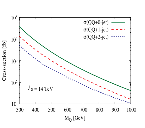
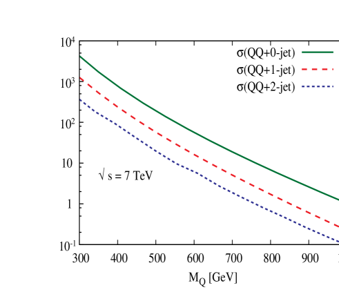
Figure 1: Pair production cross-sections of level-one KK $t$– or $b$–quarks as a function of their masses in proton proton collisions at center of mass energies 14 TeV and 7 TeV respectively. Also shown are the cross-sections for pair-production in association with one or two hard jets (see eq.6).

For numerical evaluation of the cross-sections, we use a tree-level Monte-Carlo programme incorporating CTEQ6L [22] parton distribution functions. Both the renormalization and the factorisation scales have been set equal to the subprocess center-of-mass energy $\sqrt{\hat{s}}$. The ensuing cross-sections are presented in Fig.1 for two different values of the proton-proton center of mass energy. Given the typical spectrum (displayed in Table 1), it is immediately apparent that the cross-sections for $b^{1}_{1}$-pair production would be essentially identical to those for $b^{1}_{2}$, while $t^{1}_{2}$-pair production rates would slightly exceed those for $t^{1}_{1}$. While the NLO and NLL corrections can be well estimated by a proper rescaling of the corresponding results for $t\bar{t}$ production, we deliberately desist from doing so. With the $K$-factor expected to be large [23], our results would thus be a conservative one.

At this stage, it is worthwhile to consider the possibility that the pair-production be accompanied by other hard jets. This would be of particular importance in estimating the background from $t\bar{t}$–production as discussed in the next section. Note that, nominally, the production of extra light jets is associated with soft and collinear singularities. Parts of such processes are, of course, absorbed in defining the higher-order (NLO/NNLO, as the case may be) cross-sections. Defining, somewhat arbitrarily,

$$\sigma(Q\bar{Q}+n_{j}\mbox{--jets})\equiv\sigma[p_{T}(j)>30\,{\rm GeV},\,|\eta(j)|<2.5,\,\Delta R(j-j)>0.7]$$ (6)

where the last requirement is applicable for $n_{j}\geq 2$ and serves to eliminate a particular collinear singularity by demanding a minimum distance among them in the $\eta-\phi$ plane, with $\phi$ being the azimuthal angle, and $\Delta R\equiv\sqrt{(\Delta\eta)^{2}+(\Delta\phi)^{2}}$. In Fig.1, we also plot these cross-sections $n_{j}=1,2$. For $n_{j}\geq 3$, the corresponding cross sections are too small to be of relevance. Note that the ratios $\sigma(n_{j}=1,2)/\sigma(n_{j}=0)$ actually increases marginally with $M_{Q}$. It should be realised that the simultaneous use of eq.6 alongwith $K$-factors could result in some double-counting, and, ideally one should employ higher-order monte-carlo generators. However, given the kinematic requirements we impose, the extent of this error is miniscule and this does not alter the results in any significant way.

Let us now turn our attention to the decay patterns for each of these KK-excitations. $t_{1}^{1}$ and $b_{1}^{1}$ being dominantly right-handed, have very small decay widths into $W^{1}$ and $Z^{1}$. Consequently, the $b_{1}^{1}$ decays into a $b-\gamma^{1}$ pair with almost a 100% branching ratio. However, $t^{1}_{1}\rightarrow t\gamma^{1}$ is kinematically disallowed unless $R^{-1}>1\,{\rm TeV}$. For smaller $R^{-1}$, the only allowed decay mode for the $t^{1}_{1}$ is into $H^{1+}\;b$. Similarly, kinematics dictates that $t^{1}_{2}$ decays dominantly to $W^{1}b$ and $b^{1}_{2}$ decays to $Z^{1}b$ in spite of the fact that either of these KK-quarks couple to both $W^{1}$ and $Z^{1}$.

While $\gamma^{1}$ is the LKP and hence stable (escapes detection), both $W^{1}$ and $Z^{1}$ must decay. The $Z^{1}$ is lighter than the excited quark states. Furthermore, there is no tree-level $Z^{1}Z\gamma^{1}$ coupling. Thus, the dominant decay modes of the $Z^{1}$ are into the $(L^{1})^{\pm}L^{\mp}$ and $\nu^{1}\nu$ final states with nearly equal branching ratios. In the former case, the excited lepton decays subsequently ($L^{1}\rightarrow L\gamma^{1}$). This leads to a $Z^{1}$ signal consisting of two (oppositely) charged leptons and missing energy. Kinematics does not permit the $W^{1\pm}$ to decay either hadronically or in the $W^{\pm}\gamma^{1}$ channel. Consequently, it decays to either $L^{\pm}\nu^{1}$ or to $L^{1\pm}\nu$ with equal branching ratios. The final decay products are therefore $L^{\pm}\nu\gamma^{1}$ of which only the charged leptons are observable. Hence, we have

$$\begin{array}[]{rclcl}t^{1}_{2}&\to&W^{1+}+b&\to&b+L^{+}+\nu+\gamma^{1}\\[8.61108pt] b^{1}_{2}&\to&Z^{1}+b&\to&b+\nu^{1}+\nu,\ b+L^{+}+L^{-}+\gamma^{1}\end{array}$$ (7)

Thus, $t^{1}_{2}$-pair production would dominantly lead to a pair of $b$-jets, a pair of opposite sign-leptons (not necessarily of the same flavor) and missing transverse energy. The same configuration is also reached in nearly half the events resulting from $b^{1}_{2}$-pair production. The other half of the latter case is shared roughly equally between ($2\,b+p_{T}/\hskip 4.30554pt$) and ($2\,b+4\,\ell+p_{T}/\hskip 4.30554pt$) events.

Let us also briefly comment on the possible decay of the $H^{1\pm}$, a by-product of $t^{1}_{1}$ production. As the level-1 Higgs masses may receive a substantial contribution from the boundary Higgs mass $\overline{m}_{H}$ (see eqn.5), their decay patterns are crucially dependent on this quantity. For simplicity, we have set $\overline{m}_{H}=0$ in our analysis. Given this, kinematical constraints allow only $H^{1-}\to\tau^{1}_{1}+\bar{\nu}_{\tau}$. The tiny mass separation between the LKP and $\tau^{1}_{1}$ ensures that the latter subsequently decays to a $\gamma^{1}$ and a very soft $\tau$. Such soft $\tau$’s, whether from this decay chain or produced otherwise (such as from the decays of $\tau^{1}_{2}$, which are produced from $W^{1\pm}$ or $Z^{1}$) often escape detection in a hadronic environment. So in the following analysis we will only bank on the detection of prompt $e$’s and $\mu$’s. Of course, the inclusion of a non-zero $\overline{m}_{H}$ would open other decay channels to the $H^{1\pm}$, thereby raising the possibility that some of the $t^{1}_{1}\bar{t}^{1}_{1}$ events would lead to final states observable above the SM background. This, however, would only add to the significance of our numerical results, at the cost of including an additional parameter. Once again, we desist from such a course of action.

IV Collider searches

As we have argued above, the dominant by-products of $t^{1}_{2}\,\bar{t}^{1}_{2}$ and $b^{1}_{2}\,\bar{b}^{1}_{2}$ production are a pair of $b$-quarks, a pair of oppositely charged leptons (not necessarily of the same flavor) accompanied by missing transverse energy. This, of course, constitutes a classic top-quark detection strategy. It, thus, might be tempting to search for such states at the Tevatron. However, for $R^{-1}$ allowed currently, the production rates at the Tevatron are too small to be of any relevance. Hence, we concentrate on the LHC.

With the relative mass splitting between the excited quarks and the weak gauge bosons ($Z^{1}$ and $W^{1}$) and, in turn, the mass splitting between the gauge bosons and the LKP being small, it is quite obvious that, in the rest frame of the produced excited quark, the daughters $b$ and the lepton would carry only a small fraction of its mass as momenta. This, in turn, translates to relatively small transverse momenta for them even in the laboratory frame. Thus, one should profitably concentrate on such a part of the phase space. A fruitful pursual of such a methodology requires that we examine and compare the phase space distributions for signal events as well as those of the myriad backgrounds which we discuss below.

There are several SM processes which result in final states similar to that we are interested in. Consequently, one has to find the characteristics of our signal which are distinct from the SM processes. It is needless to mention that SM $t\bar{t}$ production (at the LHC), being driven by strong interactions, offers us the biggest hurdle. Apart from the $t\bar{t}$ production, non-resonant, $b\bar{b}W^{+}W^{-}$ and $b\bar{b}ZZ$ production $(\rm{\cal O}\left(\alpha_{s}\alpha_{W}\right))$ followed by the leptonic decays of the $W(Z)$-bosons, give rise to analogous final states. Drell-Yan production of leptons in association with two light flavored jets, misidentified as $b$-jet may also contribute to the background. In the following we will discuss all of these one by one.

However, before we embark on the mission to suppress the above mentioned backgrounds, it behoves us to list the basic requirements for jets and isolated leptons to be visible as such. In this quest, it should be realized though that any detector has only a finite resolution. For a realistic detector, this applies to both energy/transverse momentum measurements as well as determination of the angle of motion. For our purpose, the latter can be safely neglected and we simulate the former by smearing the energy with Gaussian functions defined by an energy-dependent width. The latter receives corrections from many sources and are, in general, a function of the detector coordinates. We, though, choose to simplify the task by assuming a flat resolution function equating it to the worst applicable for our range of interest. To wit, we have

$$\frac{\sigma_{E}}{E}=\frac{a}{\sqrt{E}}\oplus b$$ (8)

where the errors are to be added in quadrature and

$$\begin{array}[]{rclcrclcl}a_{\ell}&=&0.05\ ,&&b_{\ell}&=&5.5\times 10^{-3}&&{\rm for~{}leptons,}\\[4.30554pt] a_{j}&=&0.80\ ,&&b_{j}&=&0.05&&{\rm for~{}partons}.\end{array}$$ (9)

Keeping in mind the LHC environment as well as the detector configurations, we demand that, to be visible, a jet or a lepton must have an adequately large transverse momentum and they are well inside the rapidity coverage of the detector, namely,

$$p_{T}({\rm jet})>30\,{\rm GeV}\ ,\qquad p_{T}({\rm lept})>15\,{\rm GeV}\ ,$$ (10)

and

$$|\eta({\rm jet})|\leq 2.5\ ,\qquad|\eta({\rm lept})|\leq 2.5\ .$$ (11)

Furthermore, we demand the leptons and jets be well seperated from each other by requiring

$$\Delta R_{\ell-j}\leq 0.4~{}{\rm and}~{}\Delta R_{j\,j}>0.7\ .$$ (12)

Among the SM backgrounds mentioned above, $t\bar{t}$ production (followed by $t\rightarrow bW$ and $W\rightarrow l\nu$) is very large, even on the imposition of eqs.(10–12). Another set of important backgrounds arise from inclusive $W$– and $Z$–production. To reduce this to manageable levels, one must impose further selection cuts. Since the only hadronic constituent of our signal is given by a pair of $b$’s, we require that there be two and only two $b$-jets satisfying eqs.(10–12). For $b$-tagging efficiency, we use $\epsilon_{b}=0.6$ for each $b$. Furthermore, the event must be characterized by a minimum missing transverse momentum defined in terms of the total visible momentum, namely,

$$\not p_{T}\equiv\sqrt{\bigg{(}\sum_{\rm vis.}p_{x}\bigg{)}^{2}+\bigg{(}\sum_{\rm vis.}p_{y}\bigg{)}^{2}}\;>30\,{\rm GeV}\ .$$ (13)

While this seemingly restricts the potential SM background to $t\bar{t}$ production, in reality, a multitude of other electroweak processes contribute too. For some of these, the hard (parton level) process does not even have a source of missing energy. For example, even a $2\,b+2\ell$ final state could potentially be associated with a missing transverse momentum simply on account of mismeasurements of the jet and lepton energies. A minimum requirement of the missing transverse momentum keeps these backgrounds well under control. The requirements summarized by Eqns.(10–13), thus, constitute our acceptance cuts.

A further requirement proves useful. Most such electroweak processes involve production of $W$ or $Z$ bosons, and these could be decimated by the simple requirement of the dijet and dilepton (in the identical-flavor case) invariant masses to be substantially away from these masses. This leads to the first of our selection cuts, namely

$$m{(\ell,\ell)}\not\in[70,100]\,{\rm GeV}$$ (14)

being applicable only to the case of final states with the oppositely charged hard leptons being of identical flavor. While it might seem appropriate to impose a similar restriction on the dijet invariant mass, we desist from doing so. For one, once we require $b$-tagging for the two hardest jets, the dominant ($t\bar{t}$) background is not characterized by any such peak in $m_{b\bar{b}}$. As for the subdominant background sources wherein the jets are the daughters of a $Z$, the other cuts suffice. And, finally, such a requirement adversely affects the signal strength as we shall see below.

Backgrounds such as inclusive $W/Z$ production (single or multiple gauge bosons) were estimated with the generator Alpgen[25] and found to be in consonance with those obtained by the ATLAS collaboration after an exhaustive detector simulation[26]. For example, after imposition of the above cuts, the contributions to the background cross-section from non-resonant $bbWW$ production (and $W$-decay) is 65 fb, whereas the contributions from $bbZZ$ and $WWjj$ production (wherein two light flavored jets are misidentified as $b$-jets) are both less than a fb. In fact, one can completely get rid of $bbZZ$ events by a cut on $m_{\ell\ell}$ (Eqn.14). Similarly, the Drell-Yan production of leptons in association with two jets (mis-identified as $b$-jets) can be reduced to virtually zero by the cuts on the transverse momentum of jets (Eqn.10), missing transverse momentum (Eqn.13) and a cut on the invariant mass of the leptons (Eqn.14). So contributions from most of the processes listed earlier in this section have been reduced to innocuous levels leaving SM $t\bar{t}$ production to dominate overwhelmingly (after imposition of the acceptance cuts this contribution is to the tune of 4.1 pb).

The latter was simulated at parton level using only the tree-level matrix elements and incorporating CTEQ6L parton distributions. However, to take into account the higher order corrections, we multiplied the rate by the appropriate $K$-factor [23]. For the subdominant backgrounds, whether these be from $t\bar{t}$ with additional hard jets (see eqn. 6) or inclusive $W/Z$-production, we do not include higher-order corrections. The consequent error is miniscule. For the signal though, we are faced with the non-availability of the higher-order calculations. Given that the production is QCD-driven, it is tempting to use the $t\bar{t}$ calculation and scale it appropriately. However, we choose to desist from this. Considering the fact that the $K$-factor for the signal events are expected to be of the same order as those for $t\bar{t}$, our results thus are conservative.

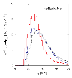
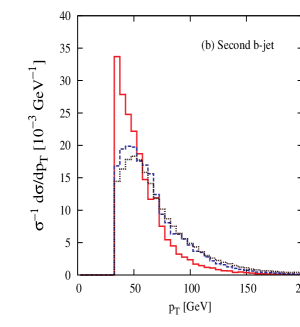
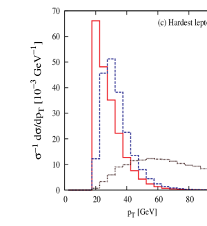
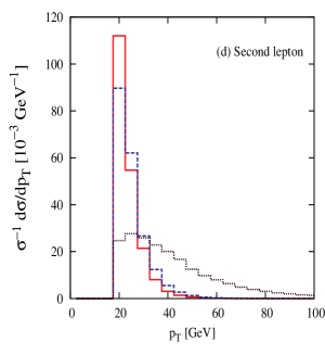
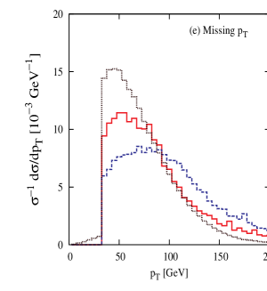
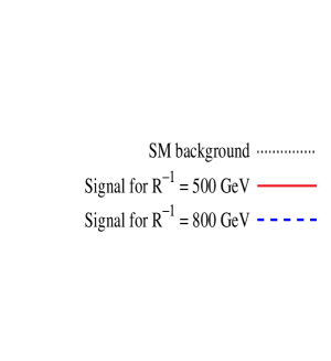
Figure 2: Normalized distributions for transverse energy on imposition of the acceptance cuts of Eqns.(10–13). (a) the leading $b$-jet, (b) the second $b$-jet, (c) the leading lepton, (d) the second lepton and (e) the missing transverse energy. Each panel shows the distributions for two signal points as well as the total SM background.

Working at $\sqrt{s}=14\,{\rm TeV}$ we present, in Figs.2(a, b), the normalized $p_{T}$ distributions for the two $b$-jets for signal events (two different values for $R^{-1}$ are used, namely 500 and 800 GeV) along with the total SM background. As expected, the signal distributions are marginally softer than the corresponding distributions for the background. This difference is less pronounced for larger $m_{Q}$ values though. However, even for $R^{-1}=800\,{\rm GeV}$, the signal $p_{T}(b)$ distribution would have been softer than the background had we limited ourselves to only the exclusive $Q\bar{Q}$ and $t\bar{t}$ events (i.e., only $n_{j}=0$ vide eq.6). More interesting—and typical to UED—are the transverse momentum distributions for the two leptons (as displayed in Figs.2(c, d)). With the signal events being peaked at a relatively small $p_{T}(\ell)$, this immediately suggests a way to suppress the widely-distributed background by imposing an upper bound on this variable, resulting in a marked improvement in the signal to noise ratio. The missing–$p_{T}$ ($\not{p_{T}}$) spectra for the signal and background are also presented in Fig.2(e). In spite of the fact that in UED a massive inivisible particle ($\gamma^{1}$) is responsible for the missing $p_{T}$ (in comparison to the SM where it is the neutrinos from various decay chains), the $\not{p_{T}}$ spectra do not differ drastically. However, it has been mentioned earlier that the cut on $\not{p_{T}}$ is very much instrumental in reducing SM backgrounds (in particular QCD driven ones) in which jet-energy/momentum mismeasurements give rise to missing transverse momentum in the final state.

The relative softness of the leptons and jets is a generic feature of the model and but a manifestation of the typically quasi-degenerate mass spectrum of UED model. Note that these are the decay products of a 1st KK-level state and that the conservation of KK-parity demands that each such decay must have another such level-one KK excitation as a daughter. The near-degeneracy of the level-one KK-spectrum thus predicts that the leptons and jets should be soft. Thus, apart from the acceptance cuts, defined above, a restriction on the maximum value of the lepton transverse momenta, would enhance the signal to background ratio considerably. As can be expected, the transverse momenta of the final state particles are correlated. For example, imposing such a restriction on the lepton transverse momenta, also renders the $p_{T}(b)$ spectra for the signal to be softer than those for the background. Thus, a similar restriction on the maximum value of the $b$-jet transverse momenta also serves to accentuate the signal.

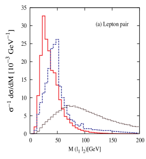
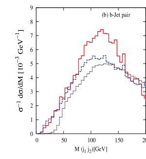
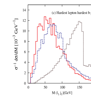
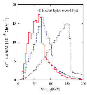
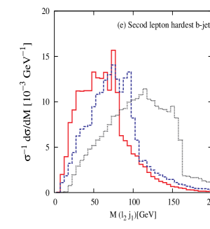
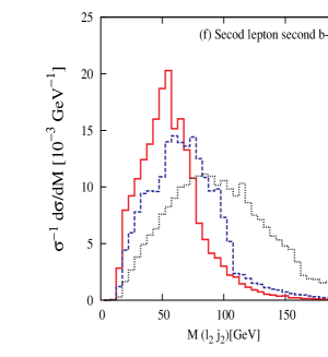
Figure 3: Normalized invariant mass distributions (on imposition of acceptance cuts only) for (a) lepton-pair, (b) $b$-jet-pair, (c) hardest lepton–hardest $b$-jet, (d) hardest lepton–second $b$-jet, (e) second lepton–hardest $b$-jet, (f) second lepton–second $b$-jet. In each case, the solid (red) and the dashed (blue) curves denote signal distributions for $R^{-1}=500(800)\,{\rm GeV}$ respectively, while the dotted (black) curve denotes the total SM background.

It is instructive to consider each of the six possible pairwise invariant mass distributions constructed out of the momenta of the two leading jets and the two leading leptons. (see Fig.3). While charge measurement for the leptons is relatively straightforward, that for the $b$’s has a relatively lower efficiency. Rather than pay the price for this, we have identified both jets and leptons by the relative magnitude of their transverse momenta. (The lepton and $b$-jet with higher (lower) $p_{T}$ are denoted by $\ell_{1}$ ($\ell_{2}$) and $b_{1}$ ($b_{2}$) respectively.) As Fig.3$a$ shows, $M(\ell_{1},\ell_{2})$ peaks at relatively small values for the signal events, while it has a flat distribution for the background. It is, thus, useful to concentrate on low $M{(\ell_{1},\ell_{2})}$ events. The $b$–$b$ invariant mass distribution (Fig.3$b$), on the other hand, is not an efficient discriminator between signal and background. Indeed, had we imposed a condition analogous to Eqn.14 for this pair, we would have lost a larger fraction of the signal than the background.

As for the various lepton–jet combinations, the sharp drop in the SM background at $M{(\ell,b)}=m_{t}$ is a kinematic effect and characteristic of the masslessness of the neutrino. The corresponding drops in the signal profiles occur at either of

$$M(\ell,b)=\frac{\sqrt{(m_{b^{1}_{2}}^{2}-m_{Z^{1}}^{2})(m_{Z^{1}}^{2}-m_{L^{1}}^{2})}}{m_{Z^{1}}}\qquad{\rm and}\qquad M(\ell,b)=\frac{\sqrt{(m_{t^{1}_{2}}^{2}-m_{W^{1}}^{2})(m_{W^{1}}^{2}-m_{\nu^{1}}^{2})}}{m_{W^{1}}}$$

depending on the particular production and decay channel involved. Given the near degeneracy of the masses, a resolution of the different steps would require a very large luminosity, and for all practical purposes, they essentially coincide. A similar feature is present in the dilepton invariant mass distribution as well and the drop occurs at

$$M(\ell_{1},\ell_{2})=\frac{\sqrt{(m_{Z^{1}}^{2}-m_{L^{1}}^{2})(m_{L^{1}}^{2}-m_{\gamma^{1}}^{2})}}{m_{L^{1}}}\ .$$

On the other hand, the $bb$ mass distribution does not show any such sharp edge (either for the signal or background) as each of the jets are decay products of two different heavy quarks, thus carrying no correlation in their mass distributions. As the structure of the bulk as well as orbifold corrections—eqs.(4, 5)—show, the relative splittings between the KK masses is always small. Thus, for the entire range of $R^{-1}$ likely to be accessible at the LHC, this drop in the signal rates would occur well to the left of the top mass. This feature, then, can be used to define further selection cuts in the form of an upper bound on such jet-lepton invariant masses, especially for the combinations of Figs.3.

Looking at the distributions in Figs. 2, 3 and following the above discussion, we are now in a position to propose a further set of cuts, which, along with Eqn.(14) constitute our selection cuts, namely

$$\begin{array}[]{rcl c rcl}p_{T}^{l}&<&50\,{\rm GeV}\\[4.30554pt] p_{T}^{b_{1}}&<&100\,{\rm GeV}&&p_{T}^{b_{2}}&<&65\,{\rm GeV}\\[4.30554pt] M(\ell_{1},\ell_{2})&<&70\,{\rm GeV}&&M(\ell_{1},b_{1})&<&100\,{\rm GeV}\\[4.30554pt] M(\ell_{1},b_{2}),M(\ell_{2},b_{1}),M(\ell_{2},b_{2})&<&75\,{\rm GeV}\end{array}$$ (15)

	Cross-section in fb after cuts					Total
					$M(l_{2},b_{1})$,	after
	Acceptance +	$p_{T}^{l}$	$p_{T}^{b_{1}}$	$M(l_{1},l_{2})$	$M(l_{2},b_{2})$,	all
Prossage	$M(l,l)$	$<50$ GeV	$<100$ GeV,	$<70$ GeV	$M(l_{1},b_{2})$	cuts
	$\in\!\!\!\!\!/$[70,100] GeV		$p_{T}^{b_{2}}$		$<75$ GeV,	in
			$<65$ GeV		$M(l_{1},b_{1})$	[fb]
					$<100$ GeV
$t\bar{t}+0$-jet	3971	1020	435.6	308	29.44
$t\bar{t}+1$-jet	668.3	182.9	84.23	72.54	8.46	38.68
$t\bar{t}+2$-jet	194.7	70.0	9.5	8.57	0.36
$bbWW$	50.6	18.13	9.31	8.3	0.42
$t_{2}^{1}\bar{t}_{2}^{1}+0$-jet	3.3	3.08	2.65	2.5	1.35
$t_{2}^{1}\bar{t}_{2}^{1}+1$-jet	1.05	1.00	0.794	0.775	0.418	1.898
$t_{2}^{1}\bar{t}_{2}^{1}+2$-jet	0.65	0.63	0.36	0.33	0.13
$b_{2}^{1}\bar{b}_{2}^{1}+0$-jet	2.81	2.63	1.26	1.26	0.34
$b_{2}^{1}\bar{b}_{2}^{1}+1$-jet	0.941	0.861	0.437	0.437	0.147	0.514
$b_{2}^{1}\bar{b}_{2}^{1}+2$-jet	0.46	0.43	0.114	0.114	0.027

Table 2: Effects of acceptance and different selection cuts applied on signal and background at the LHC with $\sqrt{s}=14$ TeV. For illustration, we have chosen $R^{-1}$ = 800 GeV for signal processes.

In Table 2, we systematically list the effects of the different cuts that we have imposed for a operating energy of $\sqrt{s}=14\,{\rm TeV}$. For illustration, we choose $R^{-1}=800\,{\rm GeV}$. It is clear that a large fraction of the background is eliminated while losing only a small part of the signal. Although further refinements are possible and a set of cuts tuned to a specific value of $R$ may be imposed (thereby improving the signal to noise ratio even further), we desist from doing so. Rather, we limit ourselves to the aforementioned cuts alone and examine the reach of the LHC experiments. Quantifying the statistical significance of the result through the use of the ratio $S\equiv N/\sqrt{N+B}$ ($N$ and $B$ being the number of signal and background events for a given luminosity), a discovery potential is nominally designated by $S>5$. In Fig.4, we present the luminosity required to obtain a $S=5$ result as a function of $R^{-1}$ at the LHC with $\sqrt{s}=14$ TeV. We conclude that, with the LHC running at a center of mass energy of 14 TeV, a 5$\sigma$ discovery is possible upto 600 (750) GeV with an integrated luminosity of $10(100){\,\rm fb}^{-1}$.

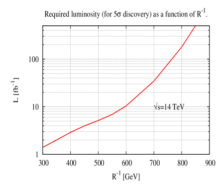
Figure 4: Required luminosities for $N/\sqrt{N+B}>5$ for a LHC run with center of mass energy 14 TeV.

For the $\sqrt{s}=7\,{\rm TeV}$ run, though, the expectations are far more modest. As Table 3 shows, the fractional reductions now are similar to those for the $\sqrt{s}=14\,{\rm TeV}$ case. However, the smaller energy means that the cross sections are smaller. Coupled with the fact that the integrated luminosity expected for such a run is smaller too, this leads to a rather modest reach.

		Cross-section in fb		Total after
Process		Acceptance Cuts +	Selection Cuts	Selection Cuts
		$M(l,l)\in\!\!\!\!\!/$[70,100] GeV		[fb]
	$t\bar{t}+0$-jet	618.6	6.23
Background	$t\bar{t}+1$-jet	99.34	1.66	7.92
	$t\bar{t}+2$-jet	21.28	0.03
	$t_{2}^{1}\bar{t}_{2}^{1}+0$-jet	10.19	5.04
Signal	$t_{2}^{1}\bar{t}_{2}^{1}+1$-jet	3.66	2.01
for	$t_{2}^{1}\bar{t}_{2}^{1}+2$-jet	1.2	0.32	7.56
$R^{-1}=250$ GeV	$b_{2}^{1}\bar{b}_{2}^{1}+0$-jet	0.36	0.18
	$b_{2}^{1}\bar{b}_{2}^{1}+1$-jet	3.2$\times 10^{-2}$	7.2$\times 10^{-3}$
	$b_{2}^{1}\bar{b}_{2}^{1}+2$-jet	1.4$\times 10^{-2}$	1.9$\times 10^{-3}$
	$t_{2}^{1}\bar{t}_{2}^{1}+0$-jet	4.61	1.93
Signal	$t_{2}^{1}\bar{t}_{2}^{1}+1$-jet	1.74	1.03
for	$t_{2}^{1}\bar{t}_{2}^{1}+2$-jet	0.58	0.14	3.54
$R^{-1}=300$ GeV	$b_{2}^{1}\bar{b}_{2}^{1}+0$-jet	0.58	0.31
	$b_{2}^{1}\bar{b}_{2}^{1}+1$-jet	0.21	0.13
	$b_{2}^{1}\bar{b}_{2}^{1}+2$-jet	3.4$\times 10^{-2}$	1.9$\times 10^{-2}$

Table 3: Signal and background cross-section after selection and acceptance cuts for the LHC with 7 TeV center-of-mass energy.

V Summary and Conclusion

Universal extra-dimensional models, which are phenomenologically interesting candidates for physics beyond the Standard Model, are characterized by towers of Kaluza Klein excitations for each of the SM particle. In the minimal version of the UED (in which we are interested in the present work), these KK states are characterized by a single positive integer $n$ known as the KK number, with a mass-separation that is almost constant. In addition, the higher-dimensional theory being necessarily non-chiral, at every KK-level, there correspond two excitations corresponding to each SM fermion (one being a $SU(2)$ doublet and the other a singlet). Conservation of KK parity stipulates both that the first-level states can only be pair-produced and that the lightest of these constitutes a stable weakly interacting massive particle ($\gamma^{1}$ in our case) and, hence, a candidate for the Dark Matter density of the universe.

In this paper, we consider the pair production of the $n=1$ KK-excitations of top and bottom quarks at the LHC. Once produced, the heavy top and bottom quarks decay to SM $b$ quarks along with $W^{1}$ and $Z^{1}$ (KK-excitations of gauge bosons). The decays of the gauge boson excitations, in turn, give rise to leptons and missing $p_{T}$ (from the undetected $\gamma^{1}$). Thus, the signal constitutes a pair of tagged $b$ jets, opposite sign di-leptons (not necessarily of the same flavour) and missing $p_{T}$. This, of course, is a classic signature for the SM top quark pair production and, hence, would be studied very well at the LHC.

While the $t\bar{t}$ (and other assorted SM) background for these final state is much larger compared to the typical signal size, we show that, with a careful choice of kinematic cuts, the signal can be enhanced vis-à-vis the background, while retaining enough signal events for a positive verdict. To be quantitative, with the LHC operating at $\sqrt{s}$ = 14 TeV, an accumulated luminosity of $10(100)\,{\rm fb}^{-1}$, would allow us to discover UED in this mode as long as $R^{-1}$ does not exceed about 600 (750) GeV. It should be emphasized here that our analysis neither takes care of all experimental effects, nor is the event selection algorithm the most optimized one. Combined with the fact that we deliberately underestimate the signal strength by not incorporating the QCD corrections (we include those for the SM backgrounds though), our analysis is thus of an exploratory nature. However, given the fact this final state would, anyway, be well studied, the positive nature of our results encourages a detailed and careful analysis of these modes with a realistic and full detector simulation. For example, it should be noted that we have not included soft initial state radiation (ISR) effects. Typically, the production of a pair of high mass particles would often be associated with the emission of an associated high–$p_{T}$ jet [28, 29]. The typical ISR for $t\bar{t}$ production would tend to be softer. This, at first sight, might seem an additional discriminant between signal and background. On the other hand, the emission of such hard jets would tend to change the $p_{T}$ profiles to an extent. However, even the inclusion of such hard jets maintains the essential difference between the signal and background profiles. Evaluation of the entire set of effects needs a detailed simulation though and we reserve it for a future study.

Finally, it should be noted that the spectrum and the couplings in UED bear some similarity to supersymmetric and many a different non-supersymmetric scenarios which contain additional gauge bosons and/or vector-like fermions. However, in UED, the SM particles and their KK partners share the same spin. This is in contrast to the supersymmetric (which may though be argued of as an extra dimension in fermion coordinates) extension of the SM, wherein the SM particles and their superpartners carry different spins. We would like to emphasize that, from an experimental point of view, UED is closer to supersymmetry. (as supersymmetry with conserved $R$-parity does contain a stable weak massive particle). To be more specific, pair production of top-squarks in MSSM and their consequent decay would produce the same signal we have discussed above. Differentiating these two new physics alternatives will have to rely on the dissimilarity in final state phase space distributions on account of the difference in the spins of particles being produced. It might be argued that for a $t^{1}_{2}$ and a top-squark of identical masses, the UED scenario would, typically, be blessed with a significantly higher event rate. While this is indeed true, the fraction of events that survive the cut is a very strong function of the mass-splitting, and in the case of supersymmetric theories, depends crucially on the details of the model. UED models, on the other hand, are relatively free of such model-dependence. Although the quantum corrections to the spectrum do depend upon the ultra-violet completion of the theory, the fractional splitting of the masses within a generation typically remains small. In particular, the nature of the $t_{2}^{1}$ and $b_{2}^{1}$ cascades, generically, remain similar to those we considered here, notwithstanding some model-dependence. A more quantitative study of how to differentiate UED from supersymmetry, following our line of analysis in the context of LHC, is beyond the scope of the present work.

Acknowledgements:  We thank Peter Skands for some very insightful comments. DC acknowledges support from the Department of Science and Technology, India under project number SR/S2/RFHEP-05/2006. The research of AD is partially supported by project no. 2007/37/9/BRNS (DAE), India and by CSIR project no. 03(1085)/07/EMR(II). KG acknowledges support from CSIR, India.

References

- [1] T. Appelquist, H. C. Cheng and B. A. Dobrescu, Phys. Rev. D 64 (2001) 035002 [arXiv:hep-ph/0012100]; H. C. Cheng, K. T. Matchev and M. Schmaltz, Phys. Rev. D 66 (2002) 056006 [arXiv:hep-ph/0205314]. .
- [2] I. Antoniadis, Phys. Lett. B 246 (1990) 377.
- [3] G. Bhattacharyya, S. K. Majee and A. Raychaudhuri, Nucl. Phys. B 793 (2008) 114 [arXiv:0705.3103 [hep-ph]].
- [4] N. Arkani-Hamed and M. Schmaltz, Phys. Rev. D 61 (2000) 033005 [arXiv:hep-ph/9903417].
- [5] G. Servant and T. M. P. Tait, Nucl. Phys. B 650 (2003) 391 [arXiv:hep-ph/0206071].
- [6] N. Arkani-Hamed, H. C. Cheng, B. A. Dobrescu and L. J. Hall, Phys. Rev. D 62 (2000) 096006 [arXiv:hep-ph/0006238].
- [7] K. Dienes, E. Dudas, and T. Gherghetta; Nucl. Phys. B 537 (1999) 47 [arXiv:hep-ph/9806292].
- [8] K. R. Dienes, E. Dudas and T. Gherghetta, Phys. Lett. B 436 (1998) 55 [arXiv:hep-ph/9803466]. For a parallel analysis based on a minimal length scenario, see S. Hossenfelder, Phys. Rev. D 70 (2004) 105003 [arXiv:hep-ph/0405127].
- [9] G. Bhattacharyya, A. Datta, S. K. Majee and A. Raychaudhuri, Nucl. Phys. B 760 (2007) 117 [arXiv:hep-ph/0608208].
- [10] P. Dey and G. Bhattacharyya, Phys. Rev. D 70 (2004) 116012 [arXiv:hep-ph/0407314]; P. Dey and G. Bhattacharyya, Phys. Rev. D 69 (2004) 076009 [arXiv:hep-ph/0309110].
- [11] P. Nath and M. Yamaguchi, Phys. Rev. D 60 (1999) 116006 [arXiv:hep-ph/9903298].
- [12] D. Chakraverty, K. Huitu and A. Kundu, Phys. Lett. B 558 (2003) 173 [arXiv:hep-ph/0212047].
- [13] A.J. Buras, M. Spranger and A. Weiler, Nucl. Phys. B 660 (2003) 225 [arXiv:hep-ph/0212143]; A.J. Buras, A. Poschenrieder, M. Spranger and A. Weiler, Nucl. Phys. B 678 (2004) 455 [arXiv:hep-ph/0306158].
- [14] K. Agashe, N.G. Deshpande and G.H. Wu, Phys. Lett. B 514 (2001) 309 [arXiv:hep-ph/0105084].
- [15] J. F. Oliver, J. Papavassiliou and A. Santamaria, Phys. Rev. D 67 (2003) 056002 [arXiv:hep-ph/0212391].
- [16] T. Appelquist and H. U. Yee, Phys. Rev. D 67 (2003) 055002 [arXiv:hep-ph/0211023].
- [17] T.G. Rizzo and J.D. Wells, Phys. Rev. D 61 (2000) 016007 [arXiv:hep-ph/9906234]; A. Strumia, Phys. Lett. B 466 (1999) 107 [arXiv:hep-ph/9906266]; C.D. Carone, Phys. Rev. D 61 (2000) 015008 [arXiv:hep-ph/9907362].
- [18] T. Rizzo, Phys. Rev. D 64 (2001) 095010 [arXiv:hep-ph/0106336]; C. Macesanu, C.D. McMullen and S. Nandi, Phys. Rev. D 66 (2002) 015009 [arXiv:hep-ph/0201300]; Phys. Lett. B 546 (2002) 253 [arXiv:hep-ph/0207269]; H.-C. Cheng, Int. J. Mod. Phys. A 18 (2003) 2779 [arXiv:hep-ph/0206035]; A. Muck, A. Pilaftsis and R. Rückl, Nucl. Phys. B 687 (2004) 55 [arXiv:hep-ph/0312186]; B. Bhattacherjee and A. Kundu, J. Phys. G 32, 2123 (2006) [arXiv:hep-ph/0605118]; B. Bhattacherjee and A. Kundu, Phys. Lett. B 653, 300 (2007) [arXiv:0704.3340 [hep-ph]]; G. Bhattacharyya, A. Datta, S. K. Majee and A. Raychaudhuri, Nucl. Phys. B 821 (2009) 48 [arXiv:hep-ph/0608208]; P. Bandyopadhyay, B. Bhattacherjee and A. Datta, [arXiv:0909.3108 [hep-ph]]; B. Bhattacherjee, A. Kundu, S. K. Rai and S. Raychaudhuri, [arXiv:0910.4082 [hep-ph]].
- [19] G. Bhattacharyya, P. Dey, A. Kundu and A. Raychaudhuri, Phys. Lett. B 628, 141 (2005) [arXiv:hep-ph/0502031]; B. Bhattacherjee and A. Kundu, Phys. Lett. B 627, 137 (2005) [arXiv:hep-ph/0508170]; A. Datta and S. K. Rai, Int. J. Mod. Phys. A 23, 519 (2008) [arXiv:hep-ph/0509277]; B. Bhattacherjee, A. Kundu, S. K. Rai and S. Raychaudhuri, Phys. Rev. D 78, 115005 (2008) [arXiv:0805.3619 [hep-ph]]; B. Bhattacherjee, Phys. Rev. D 79, 016006 (2009) [arXiv:0810.4441 [hep-ph]].
- [20] H. C. Cheng, K. T. Matchev and M. Schmaltz, Phys. Rev. D 66 (2002) 036005 [arXiv:hep-ph/0204342].
- [21] Collider Physics V. Barger and R. Phillips; Westview Press, (1996).
- [22] J. Pumplin, D. R. Stump, J. Huston, H. L. Lai, P. M. Nadolsky and W. K. Tung, JHEP 0207, 012 (2002)
- [23] M. Cacciari et al., JHEP 0809 (2008) 127, [arXiv:0804.2800 [hep-ph]].
- [24] T. Stelzer and W. F. Long, Comput. Phys. Commun. 81, 357 (1994); F. Maltoni and T. Stelzer, JHEP 0302, 027 (2003).
- [25] M. L. Mangano, M. Moretti, F. Piccinini, R. Pittau and A. D. Polosa, JHEP 0307, 001 (2003) [arXiv:hep-ph/0206293].
- [26] G. Aad et al. [The ATLAS Collaboration], arXiv:0901.0512 [Unknown].
- [27] CMS Physics Analysis Summary, CMS PAS BTV-07-003 (2008).
- [28] T. Plehn, D. Rainwater and P. Skands, Phys. Lett. B 645, 217 (2007) [arXiv:hep-ph/0510144].
- [29] J. Alwall, S. de Visscher and F. Maltoni, JHEP 0902, 017 (2009) [arXiv:0810.5350 [hep-ph]].