The Skeleton: Connecting Large Scale Structures to Galaxy Formation

Abstract

We report on two quantitative, morphological estimators of the filamentary structure of the Cosmic Web, the so-called global and local skeletons. The first, based on a global study of the matter density gradient flow, allows us to study the connectivity between a density peak and its surroundings, with direct relevance to the anisotropic accretion via cold flows on galactic halos. From the second, based on a local constraint equation involving the derivatives of the field, we can derive predictions for powerful statistics, such as the differential length and the relative saddle to extrema counts of the Cosmic web as a function of density threshold (with application to percolation of structures and connectivity), as well as a theoretical framework to study their cosmic evolution through the onset of gravity-induced non-linearities.

Over the course of the last decades, our understanding of the extragalactic universe has undergone a paradigm shift: the description of its structures has evolved from being (mostly) isolated to being multiply connected both on large scales, cluster scales and galactic scales. This interplay between large and small scales is driven in part by the scale invariance of gravity which tends to couple dynamically different processes, but also by a the strong theoretical prejudice associated with the so-called concordant cosmological model (de Bernardis, 2000). This model predicts a certain shape for the initial conditions, leading to a hierarchical formation scenario, which predicts the formation of the so-called Cosmic Web, the most striking feature of matter distribution on megaparsecs scales in the Universe. This distribution was confirmed, observationally, more than twenty years ago by the first CfA catalog (de Lapparent et al., 1986), and later by the SDSS (Adelman-McCarthy, 2008) and 2dFGRS (Cole, 2005) catalogs. On these scales, the “Cosmic Web” picture Bond et al. (1996a) relates the observed clusters of galaxies, and filaments that link them, to the geometrical properties of the initial density field that are enhanced but not yet destroyed by the still mildly non-linear evolution (Zel’Dovich, 1970). The analysis of the connectivity of this filamentary structure is critical to map the very large scale distribution of our universe to establish, in particular, the percolation properties of the Web (Colombi et al., 2000).

On intermediate scales, the paradigm shift is sustained by panchromatic observations of the environment of galaxies which illustrate sometimes spectacular merging processes, following the pioneer work of e.g. Schweizer (1982) (motivated by theoretical investigations such as Toomre and Toomre (1972)). The importance of anisotropic accretion on cluster and dark matter halo scales (Aubert et al., 2004; Aubert and Pichon, 2007; Bailin and Steinmetz, 2005) is now believed to play a crucial role in regulating the shape and spectroscopic properties of galaxies. Indeed it has been claimed (see e.g. Ocvirk et al. (2008); Dekel et al. (2008)) that the geometry of the cosmic inflow on a galaxy (its mass, temperature and entropy distribution, the connectivity of the local filaments network, etc.) is strongly correlated to its history and nature. Specifically, simulations suggest that cold streams violently feed high redshift young galaxies with a vast amount of fresh gas, resulting in very efficient star formation. One of the puzzles of galaxy formation involves understanding how galactic disks reform after minor and intermediate mergers, a process which is undoubtedly controlled by anisotropic gas inflow.

Recently, Sousbie et al. (2008a) presented a method to compute the full hierarchy of the critical subsets of a given density field. This approach connects the study of the filamentary structure to the geometrical and topological aspects of the theory of gradient flows (Jost, 2008). In this paper, we focus on the connectivity of the corresponding network. Specifically, since galaxy formation seems to be geometrically regulated by the accretion of cold gas from the LSS, how can we use the skeleton to characterize this anisotropic accretion, and predict its evolution through perturbation theory ?

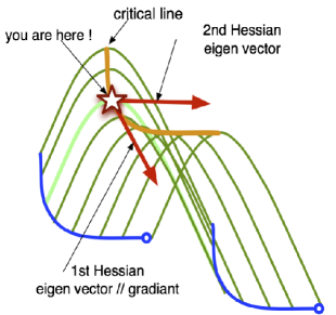
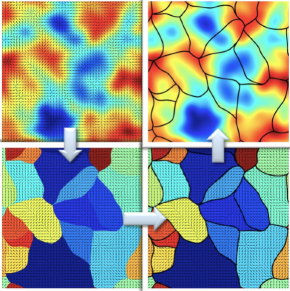
Figure 1: Left: an illustration of the local condition of the skeleton on a given ridge: on such a critical line, the gradient is parallel to the largest eigenvalue of the Hessian (corresponding to the least curvature). This defines a degenerate point process which provides means of extending the critical point theory to critical lines. Right: the fully connected skeleton algorithm illustrated in 2D. Following the panels anti-clockwise, the gradient of a given field defines neighboring regions, which correspond to the set of pixels which lead to the same minimum (a so-called void-patch). The edge of these void-patches defines a set of lines which connect critical points together: the global skeleton.

Let us first qualitatively introduce the two operating skeleton extraction algorithms, and present our findings regarding the connectivity of random fields. We will then summarize the underlying statistical theory, first for Gaussian random fields, then for non-Gaussian fields, which allows us to explain qualitatively the cosmic evolution of the connectivity of dark matter halos. In doing so we will also demonstrate how the skeleton applied to the large scale structure of the universe could be used to track $\Omega_{\rm DM}$ and $D(z)$.

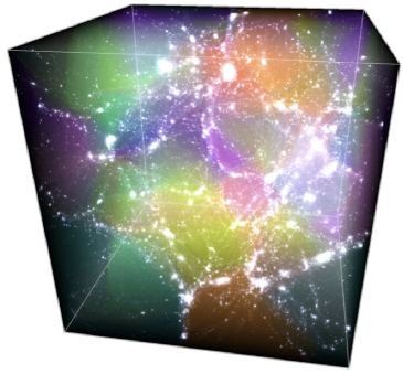
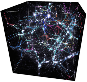
Figure 2: Left: the 3D void-patch of a simulation of the cosmological density density field in a $50h^{-1}$ Mpc box with the gadget-2 N-body code. This void-patch segmentation was computed from a $128^{3}$ pixels sampling grid smoothed over $5$ pixels ($\approx 2h^{-1}$ Mpc). Right: the corresponding skeleton. The skeleton’s different colours represent the index of the peak-patches (i.e., the void-patches of minus the density field) which provide by construction the natural segmentation of filaments attached to the different clusters.

0.1 The skeleton: algorithms

We may qualitatively define the skeleton as the 3D analog of ridges in a mountainous landscape. It consists of the special lines which connect saddles and peaks together. Mathematically these are critical solutions of the gradient flow ($\dot{r}=\nabla\rho$) between critical points. Here we want to construct such 3D ridges to trace the filaments of the large scale structures. Two venues have been explored recently: the so called local skeleton Novikov et al. (2006); Pogosyan et al. (2009a), which defines a (degenerate) point-like process corresponding to the zeros of a set of functions; the idea is that on a ridge the gradient should be along the direction of least curvature (see figure 1, left panel), which translates into the set of 3 equations:

$$\mathbf{S}\equiv\left(\nabla\nabla\rho\cdot\nabla\rho\right)\times\nabla\rho=\mathbf{0}\,,$$ (1)

where $\nabla\rho$ and $\nabla\nabla\rho$ are respectively the gradient and the Hessian of the field, $\rho$ and $\lambda_{1}>\lambda_{2}>\lambda_{3}$ its eigenvalues, with the condition $\lambda_{1}+\lambda_{2}\leq{0}$, which ensures that the critical line is a ridge. Alternative conditions on the eigenvalues of the Hessian may be applied to pick up the whole set of critical lines, see figure 3. Following Novikov et al. (2006), this local skeleton and its properties provide an alternative description to classical approaches of galaxy clustering (powerspectrum, bispectrum etc.) and attempt to achieve data compression via a mathematical description of the morphology of the cosmic web.

An alternative, global definition Novikov et al. (2006); Sousbie et al. (2008a) is to define it as the border between $N$ void-patches, where N is the dimensionality and void-patches are the attraction basins of the (anti-)gradient of the field (see figure 1, right panel in 2D, and figure 2 in 3D). The actual implemented algorithm is based on a watershed technique and uses a probability propagation scheme to improve the quality of the segmentation (see also Aragón-Calvo et al. (2007)). It can be applied within spaces of arbitrary dimensions and geometry. The corresponding recursive segmentation yields the network of the primary critical lines of the field: the fully connected skeleton that continuously link maxima and saddle-points of a scalar field together. Both constructions are of interest: the local formulation provides means of conducting detailed statistical investigation of the corresponding degenerate point-like process, while the global skeleton yields a totally connected network of lines. This critical set of lines is a compact description of the geometry of the field, richer than the knowledge of the critical points alone. For the purpose of this review, it also allows us to explore the connectivity of peaks, both from the point of view of the number of connections to other peaks, and of the number of skeleton branches leaving a given maximum. Conversely, the local skeleton formulation allows us to extend the BBKS theory Bardeen et al. (1986) of peaks in the context of critical lines to investigate their cosmic evolution, see below. Figure 3 compares the two sets of lines in the neighbourhood of a given peak.

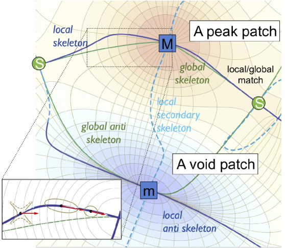
Figure 3: An example of a generic patch of a 2D field. The underlying isocontours correspond to the density field. The thin gold lines show the gradient lines of the field. The blue lines represent the local set of critical lines, given by the solution of equation (1). Primary lines are shown in solid and secondary lines are dashed. The green lines correspond to global critical lines: the skeleton and the anti-skeleton, which delineate a special bundle of gradient lines at resp. the intersection of a peak-patch and a void-patch (Jost, 2008). The primary local lines follow fairly well the gradient lines, noticeably near the saddle points, where the “stiff” approximation holds best. In contrast, the approximation worsens for the secondary critical lines. The main distinction between the global and local skeletons is that the global one follows everywhere the smooth gradient line that uniquely connects a maximum to a saddle, at the cost of deviating from being exactly on the ridge (see how in the vicinity of the minimum at the bottom, the right green line does not follow the valley). The local skeleton tries to delineate the ridges as far from extrema as possible, but then the lines that follow this local procedure from different extrema do not meet and have to rather suddenly reconnect. A particularly striking example is the loop on the right hand side. Bottom left medallion: the neighbourhood of a local critical line (thick blue line). Thin lines are isocontours of the field. Three sample points are investigated in detail. The signature, orientation and the magnitude of the local Hessian are represented by the golden shapes. Near the maximum on the right edge, the signature of the eigenvalues of the Hessian is (-1,-1), which is shown by ellipses oriented according to eigen-directions with longer semi-axis along the direction of the least curvature. At the leftmost point the eigenvalue signature is “saddle-like”, (1,-1), which is represented by a pair of hyperbolae, also oriented with respect to eigen-directions. By definition, on the critical line the gradient of the field $\nabla\rho$, shown by red arrows, is aligned with one of the eigen-directions (i.e the axis of the ellipse or hyperbola in the graph). The light cyan arrows are the tangent vectors to the critical line $\propto\boldsymbol{\epsilon}\cdot\nabla S$, while stiff approximation to them would be parallel to the gradient. The direction of the critical line is close to the gradient when it follows the ridge near the maximum, but slides at an angle in the “saddle-like” region, before joining the corresponding saddle extremal point. Note that the gradient line that takes us to the same saddle as a segment of the global skeleton (dashed green) does not follow the ridge too closely in this instance.

0.2 The skeleton: connectivity

Let us now make use of this algorithm to explore the connectivity of the corresponding network. A set of two dimensionnal Gaussian random fields (GRF) is produced, and for each of them, the peak patch and the skeleton was generated and its connectivity computed, following the second prescription described in Sousbie et al. (2008a): we chose here to smooth and label the skeleton having fixed the field extrema, (i.e. not the bifurcation points of the skeleton, see Figure 4 (top left panel)). By fixing the extrema of the field, one ensures that the skeleton subsets that link these extrema are treated independently.

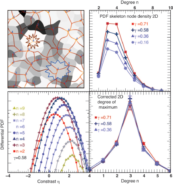
Figure 4: Top left panel: A typical (gray coded) 2D peak-patch of a Gaussian random field together with the degree of each vertex of the skeleton graph; for instance, within the red star the mean degree is 4, while the corrected degree is 3 within the blue star, as one bifurcation point is present; top right panel: the corresponding PDF of this degree, for different values of the shape parameter $\gamma$ as labeled; the mean degree is 4 and corresponds to the theoretical expectation of $2n_{\rm saddle}/n_{\rm max}$; bottom left panel: the (log) differential PDF of the degree as a function of contrast: as expected, the denser peaks are more connected; interestingly, the distribution seems Gaussian at fixed $n$ even though its marginal isn’t; bottom right panel: the corrected PDF of the number of branches connecting onto a given peak, which involves substracting the number of bifurcation points within the patch to the number of saddle points on the edge of the patch.

Let us first focus on the degree of the peakpatch, defined as the number of saddle points within a given patch which connects the skeleton of one patch to its neighbours. Hence the connectivity count reflects the number of maxima a given peak is connected to (or in the language of graph theory, the most likely degree of the vertices: $\hat{n}=\langle n\rangle$). Figure 4 (top right panel) displays this PDF as a function of $n$; in particular it allow us to compute $\langle n\rangle$, the mean $n$ which is found to be independent of $\gamma$, the shape parameter of the underlying GRF. The bottom left panel shows the corresponding normalized PDF$(n,\eta)$ versus the contrast $\eta$. As expected the number of connections increases with contrast. Indeed, near the maximum at high contrast all eigen values tend to become equal (Pichon and Bernardeau, 1999). Therefore all incoming directions become possible.

Let us now take the other (astrophysically relevant) perspective and count the actual number of filaments incident onto a given maximum. This local (intra patch) degree is in fact equal to the number of saddle points minus the number of bifurcation within the peakpatch: $n_{\rm max}=n_{\rm saddle}-n_{\rm bifurcation}\,.$ The bottom right panel of figure 4 shows the corresponding PDF($n_{\rm max}$). Note that this distribution is almost symmetrical, centered at $\langle n_{\rm max}\rangle=3$. Figure 5 (left panel) presents the same distribution in 3D, which is very skewed and presents a sharp mode at 3. Its cosmic evolution, measured in CDM dark matter simulations with and without dark energy is qualitatively shown on the right panel. Our purpose in the rest of this paper is to explain qualitatively this cosmic trend by 1) deriving the statistics of bifurcation points within each patch and 2) predicting the cosmic evolution of saddle points and peaks.

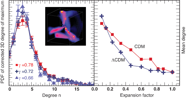
Figure 5: Left panel: the 3D corrected PDF of the number of branches connecting onto a given peak for a GRF: the mode is at 3; insert: the typical neighbourhood entropy map of a massive galaxy in the Marenostrum simulation from Dekel et al. (2008); right panel: the qualitative cosmic evolution of the mean degree in dark matter simulation with and without dark energy; as expected this degree decreases with the expansion factor as connectors get washed out by gravitationnal clustering; the rate of decrease seems sensitive to the moment when dark energy kicks in for $\Lambda$CDM models (around $a\sim 0.5$). Note that the absolute amplitude of this mean degree is not shown here as we expect the global skeleton to over estimate the mean connectivity in 3D (see main text).

0.3 The skeleton: statistics

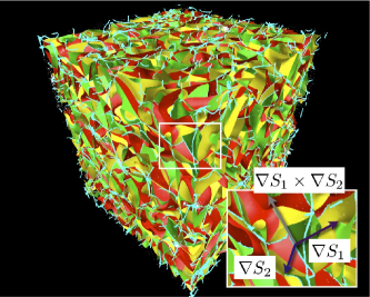
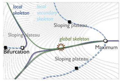
Figure 7: left panel: the local direction of the skeleton is along the cross product, $\nabla S_{1}\times\nabla S_{2}$ of the normals, $\nabla S_{1}$ and $\nabla S_{2}$, of the iso-surfaces, $S_{1}$ and $S_{2}$, defined by the critical condition (1). Hence the differential length per unit volume of the skeleton is given by expectation of the modulus of this cross product, which can be expressed locally with the JPDF of the field and its successive derivatives. right panel: the three types of singular point ($\nabla_{k}S=\mathbf{0}$) on the critical lines (in solid blue: primary; dashed: secondary; green: gradient lines of the global skeleton): an extremum (open circle), a “bifurcation” (white square), and “slopping plateaux” (black squares). The red star corresponds to what would naively correspond to the bifurcation point.

As illustrated first in 3D on Figure 7, the critical condition given by equation (1) defines 3 isosurfaces corresponding to its components, and the local skeleton direction is simply given by the cross products of two of its normals. Hence the differential length (per unit volume) is simply given by the statistical expectation

$$\frac{\partial{\cal L}}{\partial\eta}=\left(\frac{1}{R_{*}}\right)^{2}\int d^{3}x_{k}d^{6}x_{kl}d^{10}x_{klm}\ |\nabla s^{i}\times\nabla s^{j}|{P}(\eta,x_{k},x_{kl},x_{klm})\delta_{D}\left(s^{i}(x_{k},x_{kl},x_{klm})\right)\delta_{D}\left(s^{j}(x_{k},x_{kl},x_{klm})\right)\,,$$ (2)

where ergodicity allowed us to replace volume average by ensemble average over the statistical distribution, ${P}(\eta,x_{k},x_{kl},x_{klm})$, of the successive (a-dimensional) derivatives, $\sigma_{1}x_{k}\equiv\nabla_{k}\rho$, $\sigma_{2}x_{kl}\equiv\nabla_{k}\nabla_{l}\rho,$ $\sigma_{3}x_{klm}\equiv\nabla_{m}\nabla_{l}\nabla_{k}\rho$ of the field, $\rho$. The scale factor ${1}/{R_{*}}^{2}=\sigma_{2}^{2}/\sigma_{1}^{2}$ in equation (2) follows dimensionally (given $\sigma_{2}^{2}\sigma_{1}\nabla s^{i}\equiv\nabla{S}^{i}$, $\sigma_{0}\eta\equiv\rho$). Here the variances, $\sigma_{p}^{2}$, obey $\sigma_{p}^{2}={2\pi^{N/2}}/{\Gamma[N/2]}\int_{0}^{\infty}k^{2p}P(k)k^{N-1}dk$ in $N$ dimensions. (see Pogosyan et al. (2009a) for a formal derivation of equation (2)).

More generally, for ND critical lines, the N-1 independent functions $S^{i}$ that define the critical condition (1) acquire the following reduced form in the eigenframe of the Hessian of the field: $s^{i}=x_{1}x_{i}\left(\lambda_{1}-\lambda_{i}\right)=0.$ The measurements in Sousbie et al. (2008b) found that, over the range of spectral indexes relevant to cosmology, the third derivatives of the field $x_{klm}$ play a subdominant nature. In the so called “stiff” approximation we therefore omit the third derivative, effectively assuming that the Hessian can be treated as constant during the evaluation of $\nabla s$. This picture corresponds to a skeleton connecting extrema with relatively straight segments. Let us first assume that the underlying field is Gaussian. In the stiff approximation, the gradients ${s^{i}}_{k}\equiv\nabla s^{i}$ have just two non-zero components, ${s^{i}}_{1}=x_{i}\lambda_{1}(\lambda_{1}-\lambda_{i})$ (which vanishes on the critical line) and ${s^{i}}_{i}=x_{1}\lambda_{i}(\lambda_{1}-\lambda_{i})$, which shows that in this approximation we equate the direction of the line with the gradient of the field. Substituting this expression into equation (2) and integrating over $\delta_{\rm D}(s^{i})=\delta_{\rm D}(x_{i})/({x_{1}(\lambda_{1}-\lambda_{i})})$ we obtain a simple expression for the differential length of the ND-critical lines:

$$\frac{\partial{\cal L}^{\mathrm{ND}}}{\partial\eta}\propto\left(\frac{1}{R_{*}}\right)^{N-1}\frac{1}{\sqrt{1-\gamma^{2}}}\int\cdots\int\prod_{i\leq N}d\lambda_{i}\prod_{i<j}(\lambda_{i}-\lambda_{j})\left|\prod_{i>1}\lambda_{i}\right|\exp\left(-\frac{1}{2}Q_{\gamma}(\eta,\{\lambda_{i}\})\right)\,,$$ (3)

where the shape parameter $\gamma={\sigma_{1}^{2}}/{(\sigma_{0}\sigma_{2})}$ describes the correlation between the field and its second derivatives, $Q_{\gamma}$ is a quadratic form in $\lambda_{i}$ and $\eta$ which functional form is

$$Q_{\gamma}(\eta,\{\lambda_{i}\})=\eta^{2}+\frac{\left(\sum_{i}\lambda_{i}+\gamma\eta\right)^{2}}{(1-\gamma^{2})}+(N+2)\left[\frac{1}{2}(N-1)\sum_{i}\lambda^{2}_{i}-\sum_{i\neq j}\lambda_{i}\lambda_{j}\right].$$ (4)

Equation (3) simply states that the stiff differential length is the expectation of the product of the “smaller” eigenvalues, which is quite reminiscent of the classical extremal count result (the expectation of the product of all eigenvalues). It also qualitatively makes sense, as the larger the curvarture orthogonal to the skeleton, the more skeleton segment one may pack per unit volume. Since the argument of $Q_{\gamma}$ is extremal as a function of $\eta$ when $\gamma\eta\sim\sum_{i}\lambda_{i}$, the largest contribution at large $\gamma\eta$ in the integral should arise when $\lambda_{i}\propto\gamma\eta$ since near the maximum at high contrast all eigen values are equal (Pichon and Bernardeau, 1999). Hence given that $\prod_{i<j}(\lambda_{i}-\lambda_{j})$ is the measure, the only remaining contribution in the integrand comes from $\left|\prod_{i>1}\lambda_{i}\right|\propto(\lambda\eta)^{N-1}$, and the dominant term at large $\eta$ is given by

$$\frac{\partial{\cal L}^{\mathrm{ND}}}{\partial\eta}\stackrel{{\scriptstyle\gamma\eta\to\infty}}{{\sim}}\frac{1}{\sqrt{2\pi}}\exp\left[-\frac{1}{2}\eta^{2}\right]\left(\frac{\eta}{R_{0}}\right)^{N-1}\,,\quad{\rm with}\quad R_{0}=\frac{\sigma_{0}}{\sigma_{1}}\,.$$ (5)

Note that in 2D the differential length, equation (3) can be reduced to a particularly simple closed form

$$\frac{\partial{\cal L}^{\mathrm{skel}}}{\partial\eta}=\frac{1}{\sqrt{2\pi}}\exp\left[-\frac{\eta^{2}}{2}\right]\left[\frac{1}{8}\left(1+\frac{2}{\sqrt{\pi}}\gamma\eta\right)\left(1+\mathrm{Erf}\left[\frac{\gamma\eta}{\sqrt{2}\sqrt{1-\gamma^{2}}}\right]\right)+\frac{\sqrt{1-\gamma^{2}}}{2\sqrt{2}\pi}\exp\left(-\frac{\gamma^{2}\eta^{2}}{2(1-\gamma^{2})}\right)\right]\,,$$ (6)

and for the integrated skeleton length

$$L^{\mathrm{skel}}=\frac{1}{8}+\frac{\sqrt{2}}{4\pi}=0.23754~{}(\times R_{*}^{-1})\quad.$$ (7)

In other words, one expects to find one segment of skeleton per linear section of $\approx(4.2R_{*})$. Similarly, in 3D one segment of skeleton is found per surface section of $\approx(4.65R_{*}^{2})$. The match of the detailed PDF with the corresponding measurements are shown in Figure 6 in 2 and 3D. From the point of view of cosmology, the skeleton is invariant w.r.t. any monotonic bias, and traces the denser regions of the field. As shown in equations (5) and (7) its statistical description yields a measure of both $R_{*}$ and $R_{0}$, hence on the shape of the underlying powerspectrum on the corresponding smoothing scale over which the skeleton was computed. An implementation of this estimate on the SDSS catalog was carried by Sousbie et al. (2008c) and provided constraints on $\Omega_{\rm M}$.

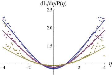
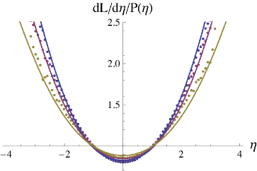
Figure 6: The relative differential length, ${\partial{\cal L}}/{\partial\eta}/\mathrm{PDF}$, measured in simulation of 2D (left) and 3D (right) Gaussian random fields with scale invariant power-law spectra versus predictions of the local theory in stiff approximation (solid curves). The spectral parameters are $\gamma=0.71,0.59,0.39$ for the 2D and $\gamma=0.77,0.70,0.60$ for the 3D simulations.

0.3.1 Bifurcation counts

In Pogosyan et al. (2009b) we conjectured that critical lines experience a qualitative change in behaviour in the vicinity of the points where either a Hessian eigenvalue orthogonal to the gradient direction vanish, or becomes equal to the one along the gradient. The first type corresponds to points where the curvature transverse to the direction of the critical line vanishes along at least one axis: typically, in 2D, they mark regions where a crest becomes a trough, or vanish into a plateau. The second type correspond to points where the critical lines would split, even though the field does not go through an extremum: a bifurcation of the lines occurs along the slope; the occasional skier or mountaineer will be familiar with a crest line splitting in two, even though the gradient of the field has not vanished. Namely, if, for definiteness, $\nabla\rho$ is taken to be along the first eigen-direction, $\lambda_{2}=0$, or $\lambda_{2}=\lambda_{1}$. We called the first case the “sloping plateau” as it designates the entering of a flat region, and the second, the “bifurcation” as it designates the places of possible reconnection of critical lines. Remarkably, these special points on the critical lines are recovered by the formal singular condition zero-tangent vector if $\nabla_{k}S^{i}$ is evaluated in the stiff approximation. Along the ND critical line defined by $x_{2}=\ldots=x_{N}=0$, the nul tangent vector condition, $x_{1}^{N-1}\prod_{i>1}\lambda_{i}\left(\lambda_{1}-\lambda_{i}\right)=0$ gives rise to three classes of situations: (i) $x_{1}=0$ corresponding to extremal points; (ii) one of $\lambda_{i}=0$ corresponding to slopping flattened tubes; and (iii) one of $\lambda_{i}=\lambda_{1}$, corresponding to an isotropic bifurcation.

To be more specific, in 2D, the skeleton’s singular points correspond to points where $S_{k}\equiv\nabla_{k}S=\mathbf{0}$. The number density, $n_{{\rm B}}(\eta)$ of singular points below the threshold $\eta$ is equal to

$$n_{{\rm B}}(\eta)=\int_{\eta>x}dxd^{2}x_{k}d^{3}x_{kl}d^{4}x_{klm}d^{5}x_{klmn}P(x,x_{k},x_{kl},\cdots)|{\rm det}\left(\nabla_{k}\nabla_{l}s\right)|\delta_{{\rm D}}(s_{1})\delta_{{\rm D}}(s_{2})\,.$$ (8)

The gradient of $S$, evaluated in the stiff approximation, in the Hessian eigenframe has the components $s_{1}^{\mathrm{stiff}}=x_{2}\lambda_{1}\left(\lambda_{1}-\lambda_{2}\right),$ and $s_{2}^{\mathrm{stiff}}=x_{1}\lambda_{2}\left(\lambda_{1}-\lambda_{2}\right),$ and involves only second derivatives of the field. Let us consider the critical line that corresponds to the $x_{2}=0$ condition in the Hessian eigenframe. Then $s_{1}^{\mathrm{stiff}}$ vanishes everywhere along this line. The requirement $s_{2}^{\mathrm{stiff}}=0$ has a solution at the extremal points, $x_{1}=0$, but also in two other cases, namely $\lambda_{2}=0$ or $\lambda_{2}=\lambda_{1}$, that we conjectured to be of interest. The second situation (isotropic Hessian) has a number density given by

$$\frac{\partial n_{\rm B}^{\rm I}}{\partial\eta}=\frac{1}{{\pi\tilde{R}}^{2}}\left[\frac{1}{\sqrt{2\pi}}\exp\left(-\frac{\eta^{2}}{2}\right)\right]\left[\frac{2}{\sqrt{2-\tilde{\gamma}^{2}}}-\frac{1}{2}(1+{\tilde{\gamma}}^{2})\right]\,,\quad{\rm with}\quad\tilde{R}=\frac{\sigma_{2}}{\sigma_{3}}\quad{\rm and}\quad{\tilde{\gamma}}=\frac{\sigma^{2}_{2}}{\sigma_{3}\sigma_{1}}\,.$$ (9)

We note that the number density of “bifurcation” points is proportional just to the PDF of the field and, consequently the bifurcation points are as frequent in the regions of high field values as in the low ones. Finally, in 3D, we expect the finite resolution bifurcation branch (connecting maxima to bifurcation points) to become bifurcation plates; in turn the boundary of these plates will be counted as critical lines by our voidpatch algorithm; we therefore expect that the algorithm numerically over estimate the degree of peakpatches. Note nonetheless that the 3D counterpart of equation (9) should allow us to correct for the number of bifurcations within each patch and compute the statistics of the number of branches connected to a given maximum.

0.3.2 Departure from Gaussianity

While the Gaussian limit provides the fundamental starting point in the study of random fields Adler (1981); Doroshkevich (1970); Bardeen et al. (1986), non-Gaussian features of the CMB and the large scale structure (LSS) fields are also of great interest. CMB inherits high level of Gaussianity from the initial fluctuations, and small non-Gaussian deviations may provide a unique window into the details of processes in the early Universe. The gravitational instability that nonlinearly maps the initial Gaussian inhomogeneities in matter density into the LSS, on the other hand, induces strong non-Gaussian features culminating in the formation of collapsed, self-gravitating objects such as galaxies and clusters of galaxies. At supercluster scales where non-linearity is mild, the non-Gaussianity of the matter density is also mild, but still essential for quantitative understanding of the filamentary Cosmic Web Bond et al. (1996a) in-between the galaxy clusters.

In order to extend the result of the previous section, following Pogosyan et al. (2009c), let us develop the equivalent of the Edgeworth expansion for the JPDF of the field variables that are invariant under coordinate rotation. Such distribution can be obtained directly from general principles: the moment expansion of the non-Gaussian JPDF corresponds to the expansion in the set of polynomials which are orthogonal with respect to the weight provided by the JPDF in the Gaussian limit. Thus, the problem is reduced to finding such polynomials for a suitable set of invariant variables. The rotational invariants that are present in the problem are: the field value $\eta$ itself, the modulus of its gradient, $q^{2}=\sum_{i}{x_{i}}^{2}$ and the invariants of the matrix of the second derivatives $x_{ij}$. A rank N symmetric matrix has N invariants with respect to rotations. The eigenvalues $\lambda_{i}$ provide one such representation of invariants, however they are complex algebraic functions of the matrix components. An alternative, more useful representation is given by the linear combination of the polynomial invariant, $I_{s}$ (where the linear invariant is the trace, $I_{1}=\sum_{i}\lambda_{i}$, the quadratic one is $I_{2}=\sum_{i<j}\lambda_{i}\lambda_{j}$ and the N-th order invariant is the determinant of the matrix. $I_{N}=\prod_{i}\lambda_{i}$) $J_{1}=I_{1}~{},J_{s\geq 2}=I_{1}^{s}-\sum_{p=2}^{s}{(-N)^{p}C_{s}^{p}}/{(s-1)/C_{N}^{p}}I_{1}^{s-p}I_{p}\,,$ where $J_{s\geq 2}$ are (renormalized) coefficients of the characteristic equation of the traceless part of the Hessian and are independent in the Gaussian limit on the trace $J_{1}$. Let us consider again here the 2D case explicitly. Introducing $\zeta=(\eta+\gamma J_{1})/\sqrt{1-\gamma^{2}}$ in place of the field value $\eta$ we find that the 2D Gaussian JPDF $G_{\rm 2D}(\zeta,q^{2},J_{1},J_{2})$, normalized over $d\zeta dq^{2}dJ_{1}dJ_{2}$, has a fully factorized form in these variables

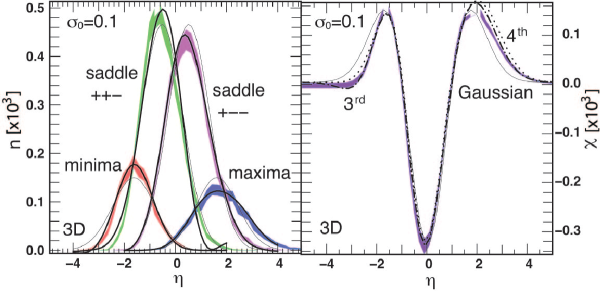
Figure 8: The number of extrema (left) and the Euler characteristic (right) for 3D gravitational collapse. In dimensional units both quantities are given per $R_{*}^{3}$ volume. The shaded bands correspond to $2\sigma$ variations over the mean measurements of 25 realizations, while the curves give the $3^{\rm rd}$ and $4^{\rm th}$ order predictions. The Gaussian prediction is shown as a thin line.

Used as a kernel for the polynomial expansion, $G_{\rm 2D}$ leads to a non-Gaussian rotation invariant JPDF in the form of the direct series in the products of Hermite ($H_{i}$), for $\zeta$ and $J_{1}$, and Laguerre ($L_{i}$), for $q^{2}$ and $J_{2}$, polynomials:

$$P_{\rm 2D}(\zeta,q^{2},J_{1},J_{2})=G_{\rm 2D}\left[1+\sum_{n=3}^{\infty}\sum_{i,j,k,l=0}^{i+2j+k+2l=n}\frac{(-1)^{j+l}}{i!\;j!\;k!\;l!}\left\langle\zeta^{i}{q^{2}}^{j}{J_{1}}^{k}{J_{2}}^{l}\right\rangle_{c}H_{i}\left(\zeta\right)L_{j}\left(q^{2}\right)H_{k}\left(J_{1}\right)L_{l}\left(J_{2}\right)\cdots\right]\,,$$ (10)

where $\sum_{i,j,k,l=0}^{i+2j+k+2l=n}$ stands for summation over all combinations of non-negative $i,j,k,l$ such that $i+2j+k+2l$ adds to the order of the expansion term $n$. A similar expression holds in 3D. The coefficients of the expansion are “centered” moments, given by the differences of the actual moments and their Gaussian limit (the latter vanishing when either $i$ or $k$ is odd): $\langle\zeta^{i}{q^{2}}^{j}{J_{1}}^{k}{J_{2}}^{l}\rangle_{c}=\langle\zeta^{i}{q^{2}}^{j}{J_{1}}^{k}{J_{2}}^{l}\rangle-(i-1)!!(k-1)!!j!l!\,.$ Once the JPDF is known it is straightforward to compute any expectation of the field which involve algebraic combinations of the invariants such as the differential length, ${\partial{\cal L}^{\mathrm{ND}}}/{\partial\eta}$ (equation (3)), extrema counts, or the Euler characteristic. For instance, the Euler characteristic can be computed completely (since there are no sign constraints on the eigenvalues of the Hessians) by noting that $I_{N}$ depends only linearly on $J_{s\geq 2}$ (e.g., $I_{3}=\left({J_{1}}^{3}-3J_{1}J_{2}+2J_{3}\right)/27$ in 3D), hence all terms in JPDF of higher order in $J_{s\geq 2}$ do not contribute. The 2D and 3D results can be combined in a very compact form if one re-expresses the “centered” moments back in terms of the field $\eta$ itself and the invariants $I_{s}$

$$\chi(\eta)=\frac{1}{2}\mathrm{Erfc}\left(\frac{\eta}{\sqrt{2}}\right)\chi(-\infty)+\frac{1}{\sqrt{2\pi}}\exp\left(-\frac{\eta^{2}}{2}\right)\times\frac{2}{(2\pi)^{N/2}}\left(\frac{\gamma}{\sqrt{N}}\right)^{N}\left[\vphantom{\sum_{i,j,k=0}^{i+2j+k=n}}H_{N-1}(\eta)+\right.$$ (11)

$$+\left.\sum_{n=3}^{\infty}\sum_{s=0}^{N}\gamma^{-s}\sum_{i,j=0}^{i+2j=n-s}\frac{(-N)^{j+s}(N-2)!!L_{j}^{(\frac{N-2}{2})}(0)}{i!(2j+N-2)!!}\left\langle\eta^{i}{q^{2}}^{j}I_{s}\right\rangle_{c}H_{i+N-s-1}(\eta)\right]\,,$$

where $i=0,s=N$ terms have been combined into the boundary term $\propto\chi(-\infty)$ fixed by the topology of the manifold, and should be omitted from the further sum. Now if the departure from Gaussianity is induced by gravitationnal clustering, the cumulants occuring in equations (10) and (11) can be computed in the context of perturbation theory Bernardeau (1992); Matsubara (1994), will scale like the growth factor $D(z)$, and can be used to constrain the dark energy equation of state via 3D galactic surveys, or shed light on the physics of the early Universe through 2D CMB maps. Regarding the connectivity, equation (11) is illustrated on figure 8 in this context. In particular, the non-linear evolution of the number of saddle points and the number of peaks is accurately predicted, which in turn should allow us to predict the mean degree, $\langle n\rangle$ of the peaks within each peak-patch given that each saddle-point connects to two peaks: $\langle n(z)\rangle=2n_{\rm saddle}(z)/n_{\rm max}(z)$. When a non-Gaussian extension of equation (9) is derived we should also be in a position to predict the non-linear evolution of the number of connecting streams on dark matter halos.

References

- de Bernardis (2000) e. a. de Bernardis, Nature 404, 955–959 (2000), arXiv:astro-ph/0004404.
- de Lapparent et al. (1986) V. de Lapparent, M. J. Geller, and J. P. Huchra, ApJ Let. 302, L1–L5 (1986).
- Adelman-McCarthy (2008) e. a. Adelman-McCarthy, ApJ Sup. 175, 297–313 (2008), arXiv:0707.3413.
- Cole (2005) e. a. Cole, MNRAS 362, 505–534 (2005), arXiv:astro-ph/0501174.
- Bond et al. (1996a) J. R. Bond, L. Kofman, and D. Pogosyan, Nature 380, 603–+ (1996a), arXiv:astro-ph/9512141.
- Zel’Dovich (1970) Y. B. Zel’Dovich, AAP 5, 84–89 (1970).
- Bond et al. (1996b) J. R. Bond, L. Kofman, and D. Pogosyan, Nature 380, 603–+ (1996b), arXiv:astro-ph/9512141.
- Colombi et al. (2000) S. Colombi, D. Pogosyan, and T. Souradeep, Physical Review Letters 85, 5515–+ (2000), arXiv:astro-ph/0011293.
- Schweizer (1982) F. Schweizer, ApJ 252, 455–460 (1982).
- Toomre and Toomre (1972) A. Toomre, and J. Toomre, ApJ 178, 623–666 (1972).
- Aubert et al. (2004) D. Aubert, C. Pichon, and S. Colombi, MNRAS 352, 376–398 (2004), arXiv:astro-ph/0402405.
- Aubert and Pichon (2007) D. Aubert, and C. Pichon, MNRAS 374, 877–909 (2007), arXiv:astro-ph/0610674.
- Bailin and Steinmetz (2005) J. Bailin, and M. Steinmetz, ApJ 627, 647–665 (2005), arXiv:astro-ph/0408163.
- Ocvirk et al. (2008) P. Ocvirk, C. Pichon, and R. Teyssier, ArXiv e-prints 803 (2008), 0803.4506.
- Dekel et al. (2008) A. Dekel, Y. Birnboim, G. Engel, J. Freundlich, T. Goerdt, M. Mumcuoglu, E. Neistein, C. Pichon, R. Teyssier, and E. Zinger, ArXiv e-prints 808 (2008), 0808.0553.
- Sousbie et al. (2008a) T. Sousbie, S. Colombi, and C. Pichon, MNRAS 1, xxx–xxx (2008a).
- Jost (2008) J. Jost, Riemannian Geometry and Geometric Analysis, Fifth Edition, Berlin ; New York : Springer, c2008., 2008.
- Aragón-Calvo et al. (2007) M. A. Aragón-Calvo, B. J. T. Jones, R. van de Weygaert, and J. M. van der Hulst, aap 474, 315–338 (2007), arXiv:0705.2072.
- Novikov et al. (2006) D. Novikov, S. Colombi, and O. Doré, MNRAS 366, 1201–1216 (2006), arXiv:astro-ph/0307003.
- Pogosyan et al. (2009a) D. Pogosyan, C. Pichon, C. Gay, S. Prunet, J. Cardoso, T. Sousbie, and S. Colombi, MNRAS 0, 0–0 (2009a).
- Bardeen et al. (1986) J. M. Bardeen, J. R. Bond, N. Kaiser, and A. S. Szalay, ApJ 304, 15–61 (1986).
- Pichon and Bernardeau (1999) C. Pichon, and F. Bernardeau, Astronomy and Astrophysics 343, 663–681 (1999), arXiv:astro-ph/9902142.
- Sousbie et al. (2008b) T. Sousbie, C. Pichon, S. Colombi, D. Novikov, and D. Pogosyan, MNRAS 383, 1655–1670 (2008b), arXiv:0707.3123.
- Sousbie et al. (2008c) T. Sousbie, C. Pichon, H. Courtois, S. Colombi, and D. Novikov, ApJ Let. 672, L1–L4 (2008c).
- Pogosyan et al. (2009b) D. Pogosyan, C. Pichon, C. Gay, S. Prunet, J. F. Cardoso, T. Sousbie, and S. Colombi, MNRAS 396, 635–667 (2009b), arXiv:0811.1530.
- Adler (1981) R. J. Adler, The Geometry of Random Fields, The Geometry of Random Fields, Chichester: Wiley, 1981.
- Doroshkevich (1970) A. G. Doroshkevich, Astrofizika 6, 581–600 (1970).
- Pogosyan et al. (2009c) D. Pogosyan, C. Gay, and C. Pichon, Phys. Rev. D 80, 081301–+ (2009c), 0907.1437.
- Bernardeau (1992) F. Bernardeau, ApJ 392, 1–14 (1992).
- Matsubara (1994) T. Matsubara, ApJ Let. 434, L43–L46 (1994).