The circumnuclear environment of the peculiar galaxy NGC 3310

Abstract

Gas and star velocity dispersions have been derived for eight circumnuclear star-forming regions (CNSFRs) and the nucleus of the spiral galaxy NGC 3310 using high resolution spectroscopy in the blue and far red. Stellar velocity dispersions have been obtained from the Caii triplet in the near-IR, using cross-correlation techniques, while gas velocity dispersions have been measured by Gaussian fits to the H$\beta$ $\lambda$ 4861 Å and [Oiii] $\lambda$ 5007 Å emission lines.

The CNSFRs stellar velocity dispersions range from 31 to 73 km s^-1. These values, together with the sizes measured on archival HST images, yield upper limits to the dynamical masses for the individual star clusters between 1.8 and 7.1 $\times$ 10⁶ M_⊙, for the whole CNSFR between 2 $\times$ 10⁷ and 1.4 $\times$ 10⁸ M_⊙, and 5.3 $\times$ 10⁷ M_⊙ for the nucleus inside the inner 14.2 pc. The masses of the ionizing stellar population responsible for the Hii region gaseous emission have been derived from their published H$\alpha$ luminosities and are found to be between 8.7 $\times$ 10⁵ and 2.1 $\times$ 10⁶ M_⊙ for the star-forming regions, and 2.1 $\times$ 10⁵ M_⊙ for the galaxy nucleus; they therefore constitute between 1 and 7 per cent of the total dynamical mass.

The ionized gas kinematics is complex; two different kinematical components seem to be present as evidenced by different line widths and Doppler shifts.

1 Introduction

The gas flows in disc of spiral galaxies can be strongly perturbed by the presence of bars, although the total disc star formation rates (SFR) do not appear to be significantly affected by them (Kennicutt, 1998a). These perturbations of the gas flow trigger nuclear star formation in the bulges of some barred spiral galaxies. External environmental influences can have strong effects on the SFR, among them, the most important by far, is tidal interactions. The young extragalactic star clusters belonging to these systems have been the aim of different studies during the last decades (e.g.  Díaz et al., 1991; Whitmore et al., 1993; Mengel et al., 2005; Bastian et al., 2005; Bastian et al., 2006; Mengel et al., 2008). The enhancement of the SFR is highly variable depending on the star formation conditions, the degree of enhancement ranging from zero in gas-poor galaxies to around 10-100 times in extreme cases (Kennicutt, 1998a). Much larger enhancements are often seen in the circumnuclear regions of strongly interacting and merging systems (Kennicutt, 1998a, b).

Yet, the bulges of some nearby, non-interacting, spiral galaxies show intense star-forming regions located in a roughly annular pattern around their nuclei. In the middle of last century, Morgan (1958) classified a sample of galaxies using as the principal classification criterion the degree of central concentration of light of each galaxy. An apparent fairly common phenomenon in some types of galaxies was pointed out by Morgan: their nuclear regions can consist of an extremely bright, small nucleus superposed on a considerably fainter background, or it may be made up of multiple “hot-spots”. Almost a decade later, Sérsic & Pastoriza (1965) suggested a relationship between the existence of a bar and the presence of abnormal features in their nuclei for a survey of bright southern galaxies. These authors extended the survey to the whole sky (Sérsic & Pastoriza, 1967), and found that $\sim$ 14 % of these galaxies presented peculiar nuclei. The distinctive nature (with respect to the more extended star formation in discs) of the luminous nuclear star-forming regions was fully revealed with the opening of the mid- and far-infrared (IR) spectral ranges (see e.g.  Rieke & Low, 1972; Harper & Low, 1973; Rieke & Lebofsky, 1978; Telesco & Harper, 1980).

In general, CNSFRs and giant Hii regions in the discs of galaxies are very much alike, although the former look more compact and show higher peak surface brightness (Kennicutt et al., 1989) than the latter. CNSFRs, with sizes going from a few tens to a few hundreds of parsecs (e.g. Díaz et al., 2000) seem to be made of several Hii regions ionized by luminous compact stellar clusters whose sizes, as measured from high spatial resolution Hubble Space Telescope (HST) images, are seen to be of only a few parsecs. Their large H$\alpha$ luminosities, typically higher than 10³⁹ erg s^-1, point to relatively massive star clusters as their ionization source. Although these Hii regions are very luminous (M_v between -12 and -17) not much is known about their kinematics or dynamics for both the ionized gas and the stars. It could be said that the worst known parameter of these ionizing clusters is their mass. As derived with the use of population synthesis models their masses suggest that these clusters are gravitationally bound and that they might evolve into globular cluster configurations (Maoz et al., 1996). Further, deeper analysis as to whether or not such cluster would survive the hostile environment of the circumnuclear regions is extremely interesting but lies outside the scope of the present work. Classically it is assumed that the system is virialized hence the total mass inside a radius can be determined by applying the virial theorem to the observed velocity dispersion of the stars ($\sigma_{\ast}$). As pointed out by several authors (e.g.  Ho & Filippenko, 1996a), at near-IR wavelengths ( 8500 Å) the contamination due to nebular lines is much smaller and since red supergiant stars, if present, dominate the light where the Caii $\lambda\lambda$ 8498, 8542, 8662 Å triplet (CaT) lines are found, these should be easily observable allowing the determination of $\sigma_{\ast}$ (Terlevich et al., 1990; Prada et al., 1994).

The equivalent width of the emission lines are lower than those shown by the disc Hii regions (see e.g.  Kennicutt et al., 1989; Bresolin & Kennicutt, 1997; Bresolin et al., 1999). Combining GEMINI data and a grid of photo-ionization models Dors et al. (2008) conclude that the contamination of the continua of CNSFRs by underlying contributions from both old bulge stars and stars formed in the ring in previous episodes of star formation (10-20 Myr) yield the observed low equivalent widths.

This is the third paper of a series to study the peculiar conditions of star formation in circumnuclear regions of early type spiral galaxies, in particular the kinematics of the connected stars and gas. In this paper we present high-resolution far-red spectra and stellar velocity dispersion measurements ($\sigma_{\ast}$) along the line of sight for eight CNSFRs and the nucleus of the spiral galaxy NGC 3310.

NGC 3310 (UGC 5786, Arp217) is a starburst galaxy classified as an SAB(r)bc by de Vaucouleurs et al. (1991), with an inclination of the galactic disc of about i $\sim$ 40 (Sánchez-Portal et al., 2000). Its coordinates are $\alpha_{\rm 2000}$=10^h 38^m 45$\aas@@fstack{s}$9, $\delta_{\rm 2000}$=+53^∘ 30′ 12″(de Vaucouleurs et al., 1991). These authors derived a distance to the galaxy equal to 15 Mpc, giving a linear scale of $\sim$ 73 pc arcsec^-1. This galaxy is a good example of an overall low metallicity galaxy, with a high rate of star formation and very blue colours. This galaxy has a ring of star forming regions whose diameter ranges from 8 ″to 12 ″and shows two tightly wound spiral arms (Elmegreen et al., 2002; van der Kruit & de Bruyn, 1976) filled with giant Hii regions. These circumnuclear regions present low metal abundance (0.2-0.4 Z_⊙ Pastoriza et al., 1993), in contrast to what is generally found in this type of objects, which show high metallicities (Díaz et al., 2007). In fact, in most cases, the [Oiii] $\lambda$ 5007 Å forbidden line can barely be seen (see e.g.  Hägele et al., 2007, 2009, hereafter Paper I and Paper II, respectively).

The ages indicated by the colours and magnitudes of the star formation regions are lower than 10 Myr (Elmegreen et al., 2002). From near-IR J and K photometry these authors derived an average age of $\sim$10⁷ yr for the large scale “hot-spots” (star forming complexes). From the observed CaT line in the Jumbo Hii region Terlevich et al. (1990) derived an age around 5 to 6 Myr. Elmegreen et al. (2002), comparing their data with Starburst99 models (Leitherer et al., 1999), estimated masses of the large “hot-spots” ranging from 10⁴ to several times 10⁵ M_⊙. They found 17 candidate super star clusters (SSCs) with absolute magnitudes between M_B = -11 and -15 mag, and with colours similar to those measured for SSCs in other galaxies (see for example Barth et al., 1995; Larsen et al., 2001).

We have measured the ionized gas velocity dispersions ($\sigma_{g}$) from high-resolution blue spectra using Balmer H$\beta$ and [Oiii] emission lines. The comparison between $\sigma_{\ast}$ and $\sigma_{g}$ on an ample sample of objects might throw some light on the yet unsolved issue about the validity of the gravitational hypothesis for the origin of the supersonic motions observed in the ionized gas in Giant Hii regions (Melnick, Tenorio-Tagle & Terlevich, 1999). In Section 2 we describe the observations and data reduction. We present the results in Section 3, the dynamical mass derivation in Section 4 and the ionizing star cluster properties in Section 5. We discuss all our results in Section 6. Finally, the summary and conclusions are given in Section 7.

2 Observations and data reduction

Table 1: Journal of Observations

Date	Slit	Spectral range	Disp.	R${}^{a}_{\rm{FWHM}}$	Spatial res.	PA	Exposure Time	seeingFWHM
		(Å)	(Å px-1)	(Å)	(″ px-1)	(o)	(sec)	(″)
2000 February 4	S1	4779-5199	0.21	12500	0.38	52	3 $\times$ 1200	1.2
2000 February 4		8363-8763	0.39	12200	0.36	52	3 $\times$ 1200
2000 February 5	S2	4779-5199	0.21	12500	0.38	100	4 $\times$ 1200	1.6
2000 February 5		8363-8763	0.39	12200	0.36	100	4 $\times$ 1200
aRFWHM = $\lambda$/$\Delta\lambda_{\rm{FWHM}}$

The data were acquired in February 2000 using the two arms of the Intermediate dispersion Spectrograph and Imaging System (ISIS) attached to the 4.2-m William Herschel Telescope (WHT) of the Isaac Newton Group (ING) at the Roque de los Muchachos Observatory on the Spanish island of La Palma. The CCD detectors EEV12 and TEK4 were used for the blue and red arms with a factor of 2 binning in both the “x” and “y” directions with resultant spatial resolutions of 0.38 and 0.36  arcsec pixel^-1 for the blue and red configurations respectively. The H2400B and R1200R gratings were used to cover the wavelength ranges from 4779 to 5199 Å ($\lambda_{c}$ = 4989 Å) in the blue and from 8363 to 8763 Å ($\lambda_{c}$ = 8563 Å) in the red with resultant spectral dispersions of 0.21 and 0.39 Å per pixel respectively, providing a comparable velocity resolution of about 13 km s^-1. A slit width of 1 arcsec was used which, combined with the spectral dispersions, yielded spectral resolutions of about 0.4 and 0.7 Å FWHM in the blue and the red, respectively, measured on the sky lines. Table 1 summarizes the instrumental configuration and observation details.

The data were processed and analyzed using iraf routines in the usual manner. Further details concerning each step can be found in Paper I. With the purpose of measuring radial velocities and velocity dispersions, spectra of 11 template velocity stars were acquired to provide good stellar reference frames in the same system as the galaxy spectra for the kinematic analysis in the far-red. They correspond to late-type giant and supergiant stars which have strong CaT features (see Díaz et al., 1989). The spectral types, luminosity classes and dates of observation of the stellar reference frames used as templates are listed in Table 2 of Paper I.

3 Results

Two different slit positions (S1 and S2) were chosen in order to observe 8 CNSFRs and the nucleus of the galaxy. One of them the conspicuous Jumbo region, labelled J, is the same region labelled R19 by Díaz et al. (2000) and region A of Pastoriza et al. (1993). Balick & Heckman (1981) dubbed it Jumbo, given its extreme luminosity (100 times more luminous in IR than 30 Dor in the Large Magellanic Cloud, Telesco & Gatley, 1984).

Fig. 1 shows the selected slits, superimposed on photometrically calibrated optical and IR images of the circumnuclear region of this galaxy acquired with the Wide Field and Planetary Camera 2 (WFPC2; PC1) and the Near-Infrared Camera and Multi-Object Spectrometer (NICMOS) Camera 2 (NIC2) on board the HST. These images have been downloaded from the Multimission Archive at STScI (MAST). The optical image was obtained through the F606W (wide V) filter, and the near-IR one, through the F160W (H). The IR image does not cover the whole circumnuclear ring, and it does not include the regions R1, R2, R7 and X. The CNSFRs have been labelled following the same nomenclature as in Díaz et al. (2000), with the nomenclature given by Pastoriza et al. (1993) for the regions in common [E for R4 and A for R19 (the main knot of the Jumbo region)] within parentheses. In both studies the regions observed are identified on the H$\alpha$ maps. We have also downloaded the F658N narrow band image (equivalent to H$\alpha$ filter at the redshift of NGC 3310) taken with the HST Advanced Camera for Surveys (ACS), shown in Fig. 2. The plus symbols in both panels of Fig. 1 and in Fig. 2 represent the position of the nucleus as given by Falco et al. (1999).

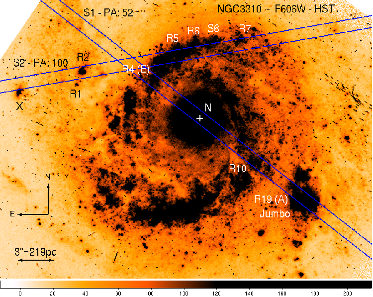
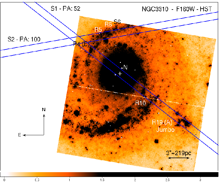
Figure 1: Left: F606W (wide V) image centred on NGC 3310 obtained with the WFPC2 camera (PC1) of the HST. Right: HST-NICMOS (NIC2) image obtained through the F160W filter. For both images the orientation is north up, east to the left. The location and P.A. of the WHT-ISIS slit positions, together with identifications of the CNSFRs extracted, are marked.

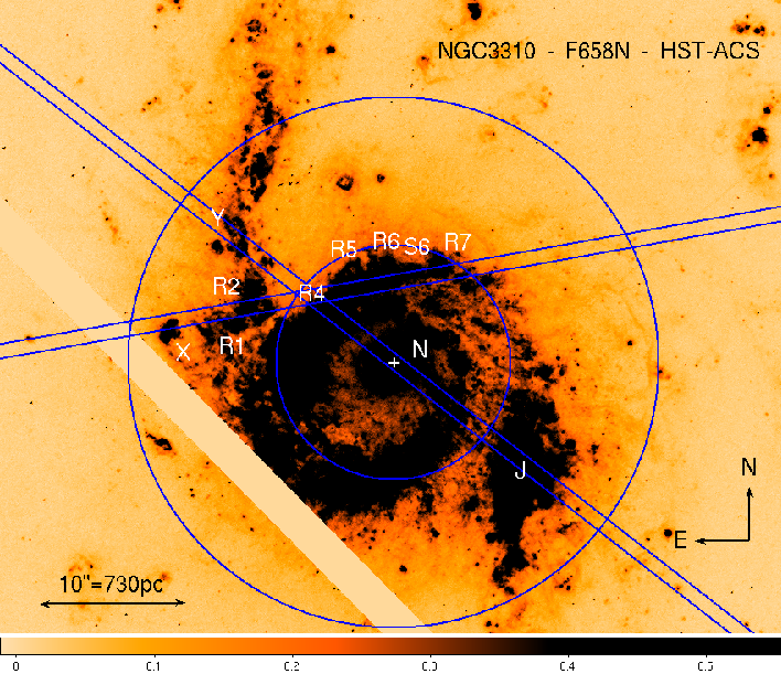
Figure 2: F658N (narrow-band [Nii] filter, at the redshift of NGC 3310, z = 0.0033 (Haynes et al. 1998), equivalent to the H$\alpha$ narrow band filter) image centred on the galaxy obtained with the ACS camera of the HST. The orientation is north up, east to the left. The location and P.A. of the WHT-ISIS slit positions, together with identifications of the CNSFRs extracted, are marked. The radii of the circles, centred at the position of the nucleus, are 8 and 18 ″.

Fig. 3 shows the spatial profiles in the H$\beta$ and [Oiii] 5007 Å emission lines (upper and middle panels) and the far-red continuum (lower panel) along each slit position. Due to the presence of intense regions (J in the blue and the galaxy nucleus in the red range in the case of S1, and R5+R4 in the blue range for S2) the profile details are very difficult to appreciate, therefore we show some enlargements of these profiles in Fig. 4. In all cases, the emission line profiles have been generated by collapsing 11 pixels of the spectra in the direction of the resolution at the central position of the lines in the rest frame, $\lambda$ 4861 and $\lambda$ 5007Å respectively, and are plotted as dashed lines. Continuum profiles were generated by collapsing 11 resolution pixels centred at 11 Å to the blue of each emission line and are plotted as dash-dotted lines. The difference between the two, shown by a solid line, corresponds to the pure emission. The far-red continuum has been generated by collapsing 11 pixels centered at $\lambda$ 8620Å.

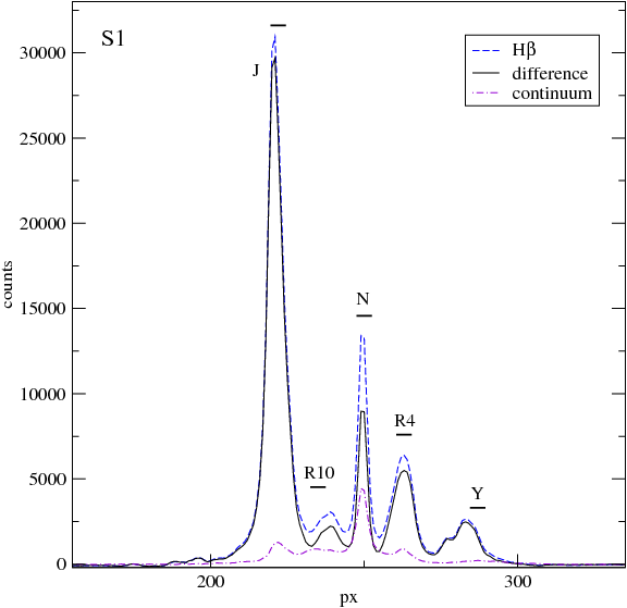
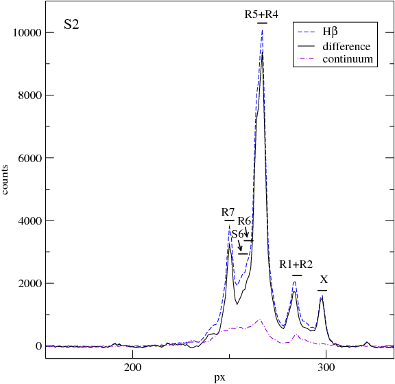
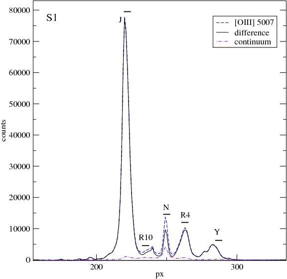
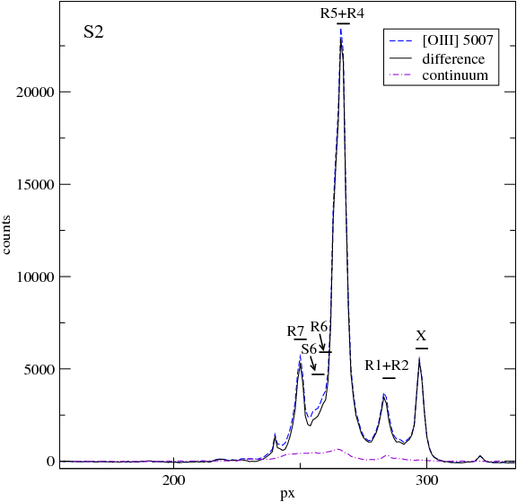
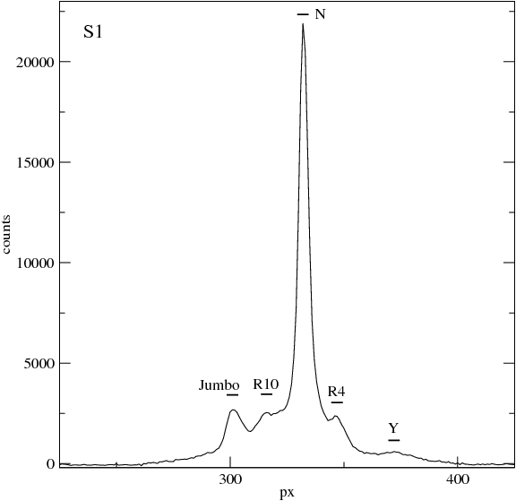
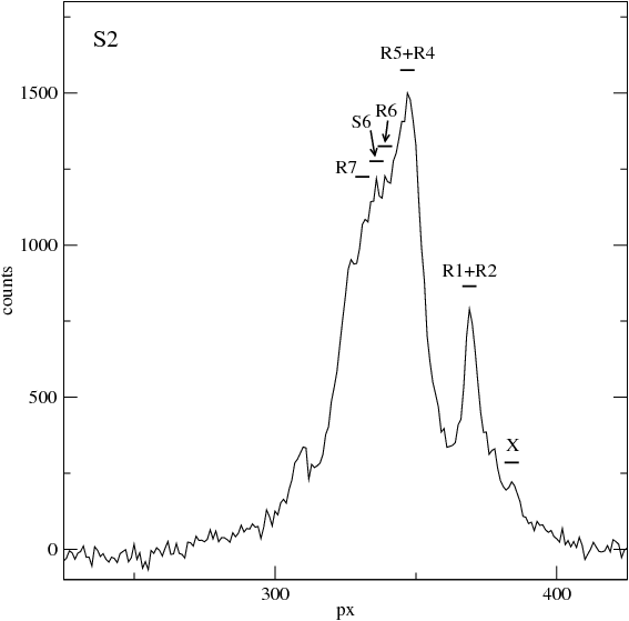
Figure 3: Spatial profiles of H$\beta$, [Oiii] $\lambda$ 5007Å and the far red (upper, middle and lower panels respectively) for each slit. For the emission lines, the profiles correspond to line+continuum (dashed line), continuum (dashed-dotted line) and the difference between them (solid line), representing the pure emission from H$\beta$ and [Oiii] respectively. For the far red profiles, the solid lines represent the continuum. Pixel number increases to the North. Horizontal small lines show the location of the CNSFRs and nuclear apertures.

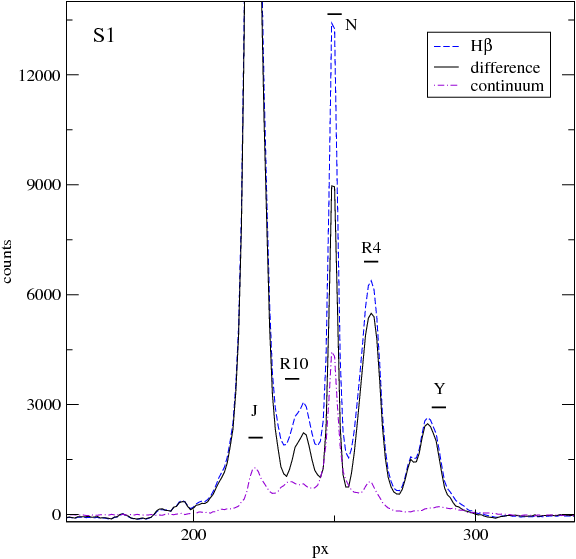
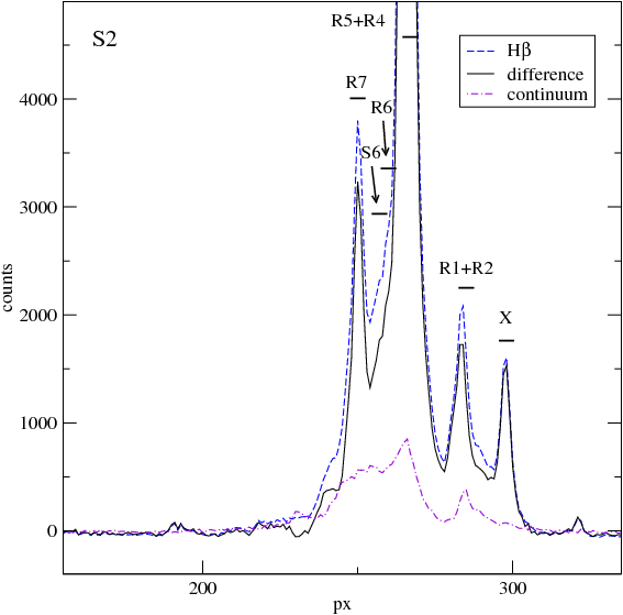
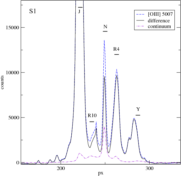
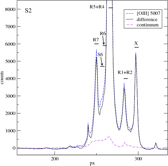
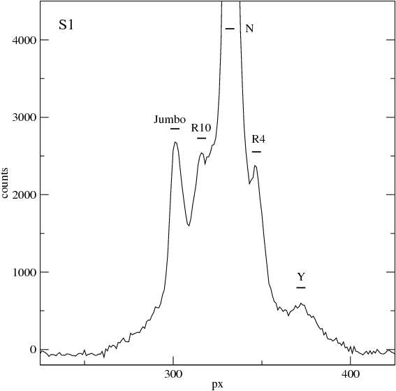
Figure 4: Enlargement of the spatial profiles presented in Fig. 3, except in the far red range of S2.

The regions of the frames to be extracted into one-dimensional spectra corresponding to each of the identified CNSFRs, were selected on the continuum emission profiles both in the blue and in the red. These regions are marked by horizontal lines and labelled in the corresponding Figures. In the H$\beta$ profiles we find two almost pure emission knots, one for each slit position, labelled Y and X by us (see Fig. 2), respectively. The former of these regions seems to be located at the tip of one vertical arm formed by pure emission regions, since it can be easily appreciable in the H$\alpha$ image from the ACS (Fig. 2) but it is almost invisible in the WFPC2-PC1 V-band image (see Fig. 1).

The spectra in slit position S2 are extracted from the circumnuclear regions located to the North and North-West of the nucleus, and therefore any contribution from the underlying galaxy bulge is difficult to assess. Slit position S1 crosses the galactic nucleus. This can be used to estimate the underlying bulge contribution. For the blue spectra, it turns out to be almost negligible amounting to, at most, 10 per cent at the H$\beta$ line. For the red spectra, the bulge contribution is more important. From Gaussian fits to the $\lambda$ 8620 Å continuum profile of S1 we find it to be about 25 per cent for R4, the weakest region, and the one closest to the nucleus. On the other hand, the analysis of the broad near-IR HST-NICMOS images shown in Fig. 1 shows less contrast between the emission from the regions and the underlying bulge which is very close to the image background emission. Its contribution is about 25 per cent for the weak regions in the central zone of NGC 3310, that is in very good agreement with the cluster identification made by Elmegreen et al. (2002) using the equivalent J and K-band HST-NICMOS images and the ground base data from KPNO (J and K-bands).

Fig. 5 shows the spectra of the observed circumnuclear regions split into two panels corresponding to the blue and the red spectral ranges. The spectrum of the nucleus of NGC 3310 is shown in Fig. 6. The blue spectra show the Balmer H$\beta$ recombination line and the collisionally excited [Oiii] lines at $\lambda\lambda$ 4959, 5007 Å. Generally, these forbidden lines are very weak (see for example Figs. 5 of Papers I and II), and, in some cases, only the strongest $\lambda$ 5007 Å is detected (right-hand panels of these Figs.). However, in the case of NGC 3310 they are very strong, due to the low abundance of the CNSFRs in this galaxy, with values between 0.2-0.4 Z_⊙ (Pastoriza et al., 1993). These low values of the abundances can be explained by the probably unusual interaction history of the galaxy (Elmegreen et al., 2002; Kregel & Sancisi, 2001; Mulder & van Driel, 1996; Smith et al., 1996; Balick & Heckman, 1981), fuelling the ring with accreted neutral gas, as modeled by Athanassoula (1992) and Piner et al. (1995). The red spectra show the stellar CaT lines in absorption. In some cases these lines are contaminated by Paschen emission which occurs at wavelengths very close to those of the CaT lines. Other emission features, such as Oi $\lambda$ 8446, [Clii] $\lambda$ 8579, Pa 14 and [Feii] $\lambda$ 8617 are also present. In Fig. 5 we can easily appreciate, for example in R4+R5, the Paschen series from Pa13 to Pa22, as well as the previously mentioned lines of O, Cl and Fe. In all cases, a single Gaussian fit to the emission lines was performed and the lines were subsequently subtracted (see also Östlin et al., 2004; Cumming et al., 2008) after checking that the theoretically expected ratio between the Paschen lines was satisfied. The observed red spectra are plotted with a dashed line. The solid line shows the subtracted spectra.

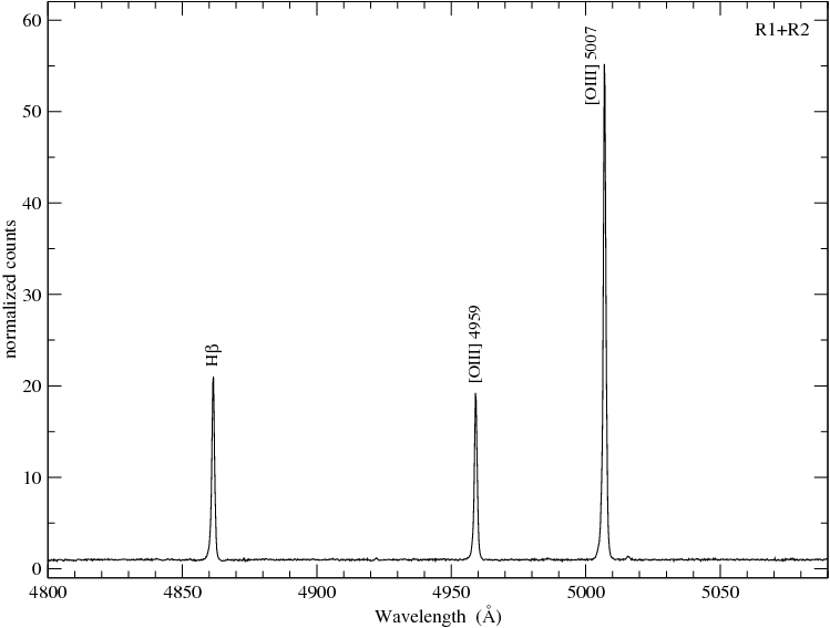
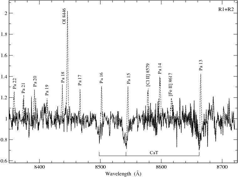
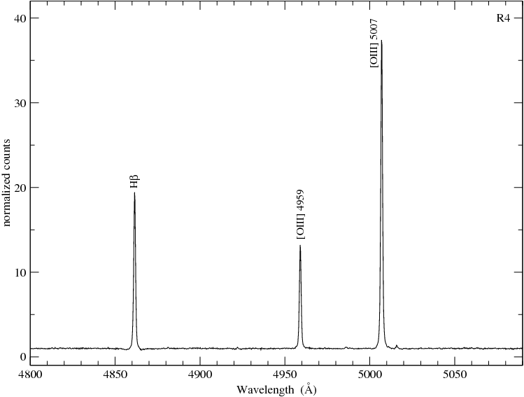
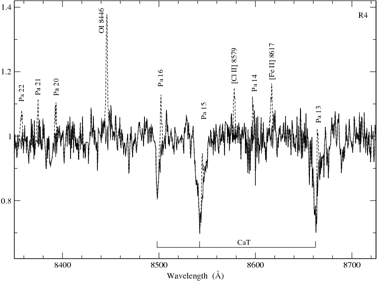
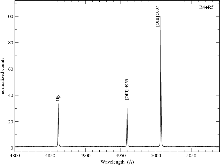
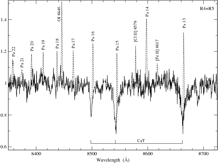
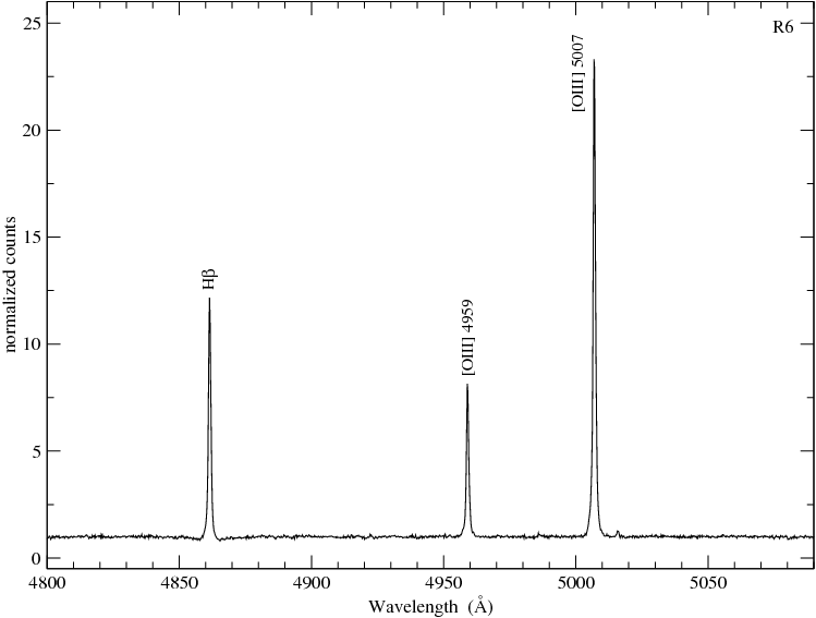
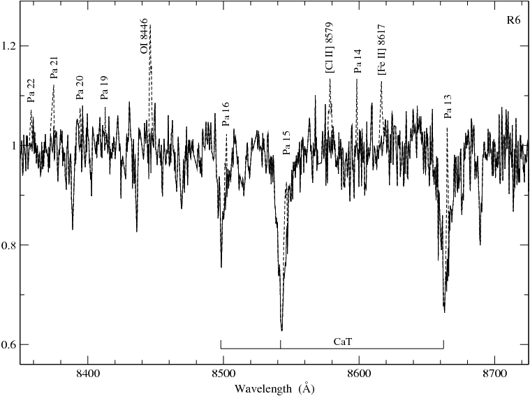
Figure 5: Blue (left) and red (right) rest frame normalized spectra of the observed CNSFRs. For the red range, the dashed line shows the observed spectrum; the solid line represents the spectrum after subtracting the emission lines (see text).

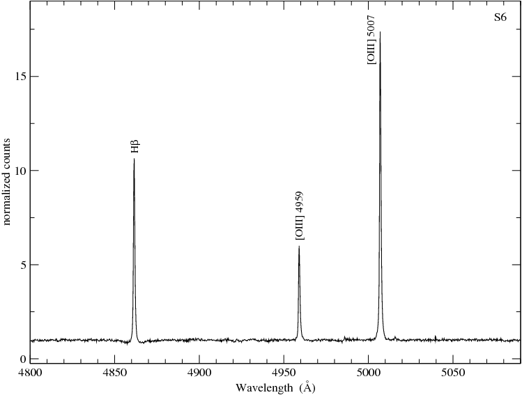
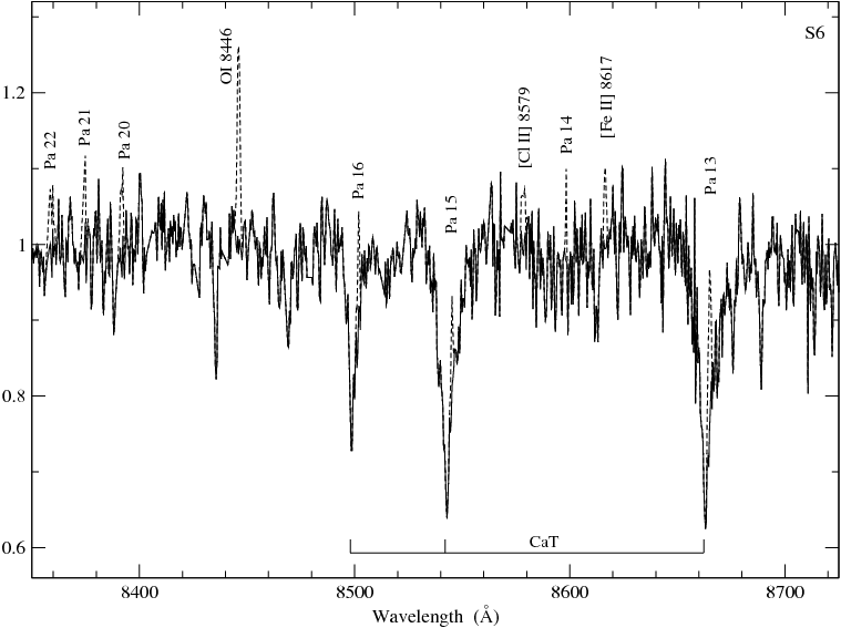
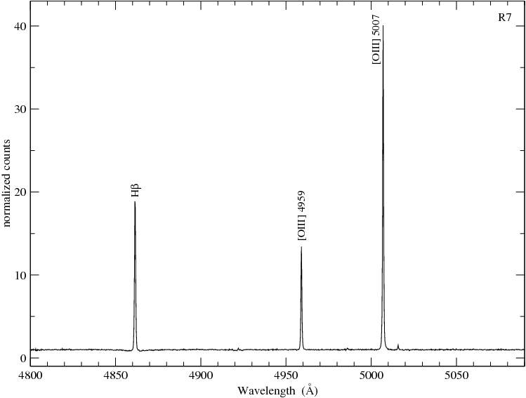
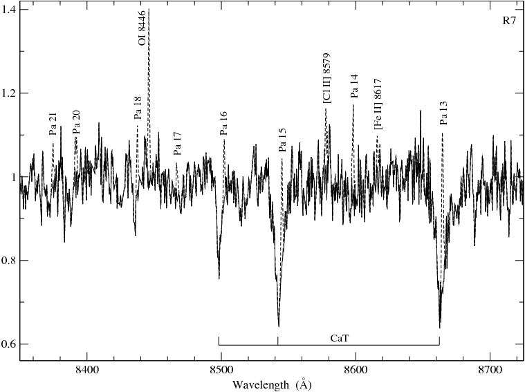
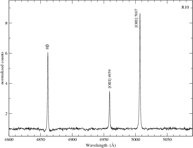
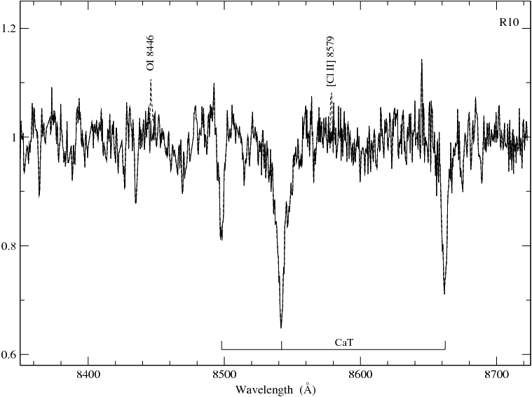
Figure 5: (cont) Blue (left) and red (right) rest frame normalized spectra of the observed CNSFRs. For the red range, the dashed line shows the observed spectrum; the solid line represents the spectrum after subtracting the emission lines (see text).

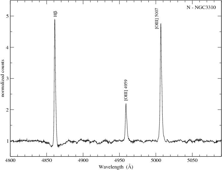
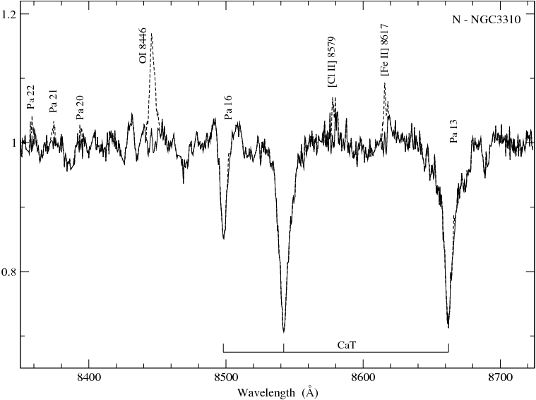
Figure 6: Blue (left) and red (right) rest frame normalized spectra of the nucleus. In the red range, the dashed line shows the observed spectrum; the solid line represents the spectrum after subtracting the emission lines (see text).

Fig. 7 shows the spectra of the almost pure emission knots labelled X and Y, and those of the Jumbo region. In all cases the blue range of the spectrum presents very intense emission lines. The red spectral range presents a very weak and noisy continuum. In the case of region X only noise is detected therefore no spectrum is shown in Fig. 7. In the other two regions we can see a set of emission lines. The Jumbo region presents many strong lines, even He and Ni in emission. Due to the low signal-to-noise ratio of the continuum and the presence of the strong emission lines in these regions of NGC 3310, we could not obtain stellar spectra with enough signal in the CaT absorption feature to allow an accurate measurement of velocity dispersions.

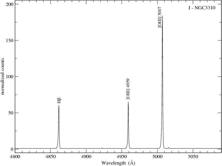
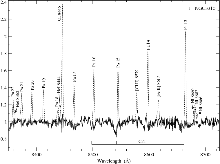
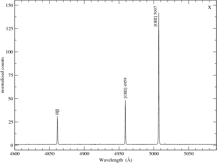
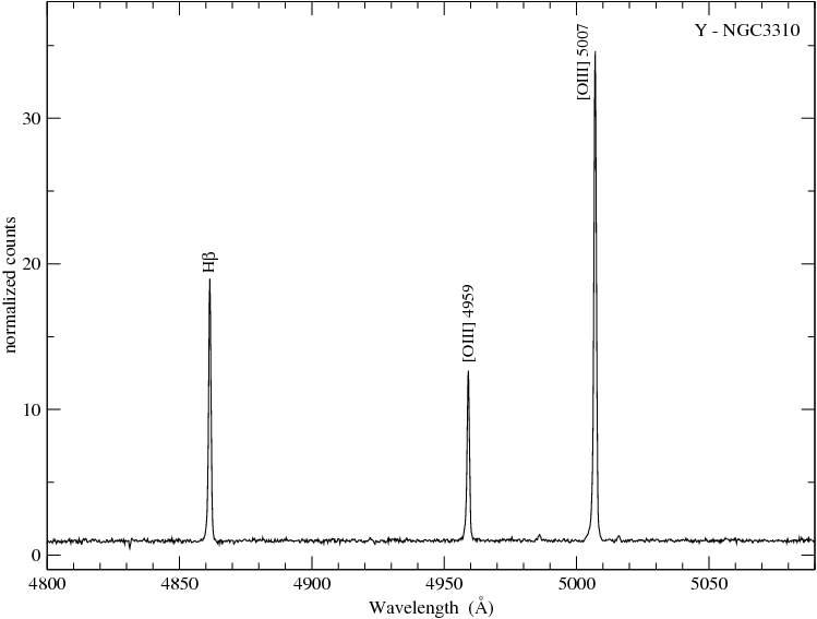
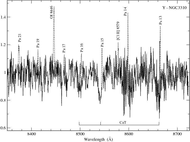
Figure 7: Idem as Fig. 5 for regions J, X (only blue) and Y. The dashed line shows the observed spectrum; the solid line represents the spectrum after subtracting the emission lines (see text).

3.1 Kinematics of stars and ionized gas

A detailed description of the methods and techniques used to derive the values of radial velocities and velocity dispersions as well as sizes, masses and emission line fluxes has been given in Paper I. Therefore only a brief summary is given below.

Stellar analysis

Stellar radial velocities and velocity dispersions were obtained from the CaT absorption lines using the cross-correlation technique, described in detail by Tonry & Davis (1979). This method requires the comparison with a stellar template that represents the stellar population that best reproduces the absorption features. This has been built from a set of 11 late-type giant and supergiant stars with strong CaT absorption lines. We have followed the work by Nelson & Whittle (1995) with the variation introduced by Palacios et al. (1997) of using the individual stellar templates instead of an average. This procedure will allow us to correct for the known possible mismatches between template stars and the region composite spectrum. The implementation of the method in the external package of iraf xcsao (Kurtz & Mink, 1998) has been used.

To determine the line-of-sight stellar velocity and velocity dispersion along each slit, extractions were made every two pixels for slit position S1 and every three pixels for slit position S2, with one pixel overlap between consecutive extractions in this latter case. In this way the S/N ratio and the spatial resolution were optimized. Besides, the stellar velocity dispersion was estimated at the position of each CNSFR and the nucleus using an aperture of five pixels in all cases, which corresponds to 1.0 $\times$ 1.8 arcsec². The velocity dispersion ($\sigma$) of the stars ($\sigma_{\ast}$) is taken as the average of the $\sigma$ values found for each stellar template, and its error is taken as the dispersion of the individual values of $\sigma$ and the rms of the residuals of the wavelength fit. These values are listed in column 3 of Table 2 along with their corresponding errors. Stellar velocity dispersions of X, Y and the Jumbo region could not be estimated due to the low signal-to-noise ratio of the continua and the CaT absorption features. The same is true for region R1+R2, where the red continuum and the CaT features after subtracting the emission lines have a low signal-to-noise ratio, although an estimate of the stellar velocity dispersion could be given in this case.

Table 2: Velocity dispersions.

			1 component		2 components
					narrow		broad
Region	Slit	$\sigma_{\ast}$	$\sigma_{gas}$(H$\beta$)	$\sigma_{gas}$([Oiii])	$\sigma_{gas}$(H$\beta$)	$\sigma_{gas}$([Oiii])	$\sigma_{gas}$(H$\beta$)	$\sigma_{gas}$([Oiii])	$\Delta$vnb
R1+R2	S2	80:	33$\pm$4	31$\pm$4	24$\pm$5	22$\pm$5	54$\pm$7	50$\pm$4	-10
R4	S1	36$\pm$3	34$\pm$3	32$\pm$3	28$\pm$4	26$\pm$3	55$\pm$5	52$\pm$4	10
R4+R5	S2	38$\pm$3	27$\pm$4	22$\pm$3	22$\pm$4	18$\pm$3	46$\pm$5	40$\pm$2	15
R6	S2	35$\pm$5	30$\pm$3	28$\pm$3	23$\pm$3	21$\pm$3	54$\pm$7	56$\pm$3	0
S6	S2	31$\pm$4	27$\pm$3	26$\pm$3	20$\pm$3	19$\pm$3	47$\pm$4	47$\pm$3	10
R7	S2	44$\pm$5	21$\pm$5	17$\pm$4	18$\pm$4	14$\pm$3	41$\pm$4	36$\pm$3	0
R10	S1	39$\pm$3	38$\pm$3	40$\pm$3	26$\pm$2	26$\pm$3	54$\pm$2	59$\pm$4	-20
N	S1	73$\pm$3	55$\pm$3	66$\pm$3	35$\pm$3	35$\pm$3	73$\pm$3	83$\pm$4	20
J	S1	—	34$\pm$2	30$\pm$2	25$\pm$2	22$\pm$2	61$\pm$3	57$\pm$3	-25
X	S2	—	22$\pm$4	18$\pm$3	18$\pm$4	14$\pm$3	40$\pm$5	30$\pm$3	-5
Y	S1	—	28$\pm$3	28$\pm$3	22$\pm$4	25$\pm$3	44$\pm$4	61$\pm$5	10
velocity dispersions in km s-1

The radial velocities have been determined directly from the position of the main peak of the cross-correlation of each galaxy spectrum with each template in the rest frame. The average of these values is the final adopted radial velocity.

Ionized gas analysis

The velocity dispersion of the ionized gas was estimated for each observed CNSFR and for the galaxy nucleus from Gaussian fits to the H$\beta$ and [Oiii] $\lambda$ 5007 Å emission lines using five pixel apertures, corresponding to 1.0 $\times$ 1.9 arcsec². For a single Gaussian fit, the position and width of a given emission line is taken as the average of the fitted Gaussians to the whole line using three different suitable continua (Jiménez-Benito et al., 2000), and their errors are given by the dispersion of these measurements taking into account the rms of the wavelength calibration. In all the studied regions, however, the best fit for the emission lines are obtained with two different components having different radial velocities of up to 25 km s^-1. The radial velocities found for the narrow and broad components of both H$\beta$ and [Oiii], are the same within the errors. An example of the two-Gaussian fit for R4+R5 in S2 is shown in Fig. 8.

For each CNSFR, the gas velocity dispersion for the H$\beta$ and [Oiii] $\lambda$ 5007 Å lines derived using single and double line Gaussian fits, and their corresponding errors are listed in Table 2. Columns 4 and 5, labelled ‘One component’, give the results for the single Gaussian fit. Columns 6 and 7, and 8 and 9, labelled ‘Two components - Narrow’ and ‘Two components - Broad’, respectively, list the results for the two component fits. The last column of the table, labelled $\Delta$v_nb, gives the velocity difference between the narrow and broad components. This is calculated as the average of the H$\beta$ and [Oiii] fit differences. Taking into account the errors in the two component fits, the errors in these velocity differences vary from 5 to 10 km s^-1.

We have also determined the distribution along each slit position of the radial velocities and the velocity dispersions of the ionized gas using the same procedure as for the stars, that is using spectra extracted every two pixels for S1 and every three pixels, superposing one pixel for consecutive extractions, for S2. These spectra, however, do not have the required S/N ratio to allow an acceptable two-component fit, therefore a single-Gaussian component has been used. The goodness of this procedure is discussed in Section 4 below.

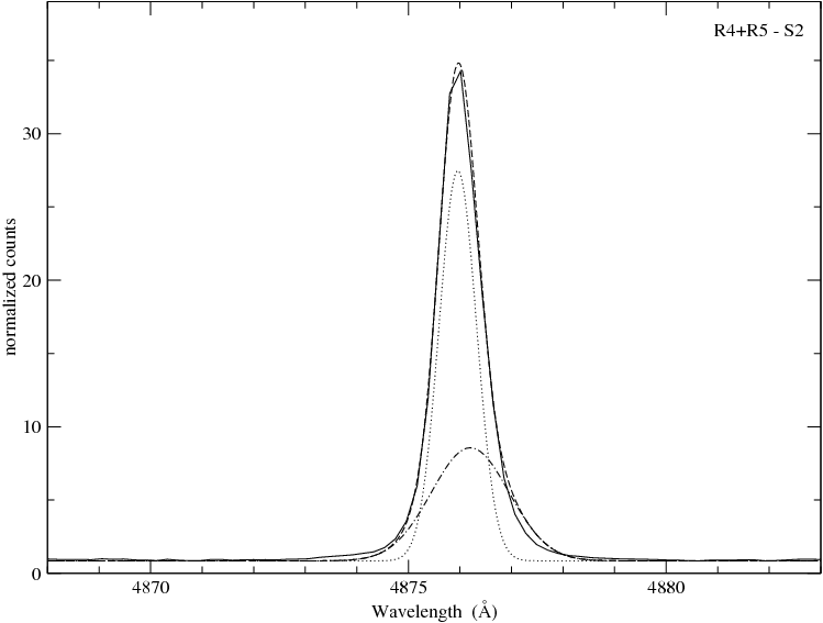
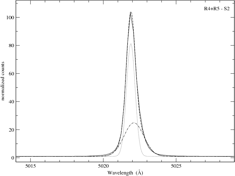
Figure 8: Sections of the normalized spectrum of R4+R5 (solid line). The left panel shows from 4868 to 4883 Å containing H$\beta$ and the right panel shows from 5014 to 5029 Å containing the [Oiii] $\lambda$ 5007 Å emission line. For both we have superposed the fits from the ngaussfit task in iraf; the dashed-dotted line is the broad component, the dotted line is the narrow component and the dashed line is the sum of both.

3.2 Emission line ratios

We have used two different ways to integrate the intensity of a given line: (1) if an adequate fit was attained by a single Gaussian, the emission line intensities were measured using the splot task in iraf. For the H$\beta$ emission lines a conspicuous underlying stellar population is inferred from the presence of absorption features that depress the lines (e.g. see discussion in Díaz, 1988). Examples of this effect can be appreciated in Fig. 9. We have defined a pseudo-continuum at the base of the line to measure the line intensities and minimize the errors introduced by the underlying population (for details see Hägele et al., 2006). (2) When the optimal fit was obtained by two Gaussians the individual intensities of the narrow and broad components are estimated from the fitting parameters (I = 1.0645 A $\times$ FWHM = $\sqrt{2\pi}$ A $\sigma$; where I is the Gaussian intensity, A is the amplitude of the Gaussian, FWHM is the full width at half-maximum and $\sigma$ is the dispersion of the Gaussian). A pseudo-continuum for the H$\beta$ emission line was also defined in these cases. The statistical errors associated with the observed emission fluxes have been calculated with the expression $\sigma_{l}$ = $\sigma_{c}$N^1/2[1 + EW/(N$\Delta$)]^1/2, where $\sigma_{l}$ is the error in the observed line flux, $\sigma_{c}$ represents the standard deviation in a box near the measured emission line and stands for the error in the continuum placement, N is the number of pixels used in the measurement of the line intensity, EW is the line equivalent width and $\Delta$ is the wavelength dispersion in Å pixel^-1 (González-Delgado et al., 1994). For the H$\beta$ emission line we have doubled the derived error, $\sigma_{l}$, in order to take into account the uncertainties introduced by the presence of the underlying stellar population (Hägele et al., 2006).

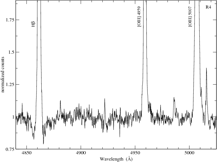
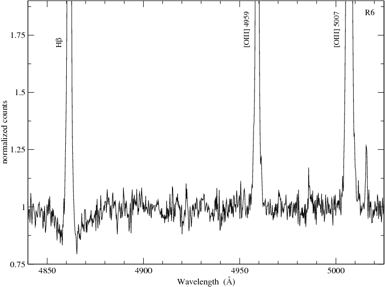
Figure 9: Enlargement of the blue rest frame normalized spectra of R4 (left) and R6 (right).

The logarithmic ratio between the emission line intensities of [Oiii] $\lambda$ 5007 Å and H$\beta$ and their corresponding errors are presented in Table 3. We have also listed the logarithmic ratio between the emission line fluxes of [Nii] $\lambda$ 6584 Å and H$\alpha$ together with their corresponding errors. These values listed for R4, R4+R5, S6, J and the nucleus are from Pastoriza et al. (1993; S6 seems to be their region L). For the rest of the regions we used an extrapolation of the results given by them from the spatial profiles of these emission lines. They reported a constant value of 0.2 for the [Nii] / H$\alpha$ ratio for the Hii regions in their slit positions 2 and 3, while this value changes from 0.2 to 0.5 along position 1 over the nucleus of the galaxy, being 0.23 and 0.27 for regions B and L, respectively. We adopt for R1+R2, R6, R7, R10, X and Y, a value of 0.2 without assigning any error to it.

Table 3: Line ratios.

		One component	Two components
			Narrow	Broad
Region	Slit	log([Oiii]5007/H$\beta$)	log([Oiii]5007/H$\beta$)	log([Oiii]5007/H$\beta$)	log([Nii]6584/H$\alpha$)a
R1+R2	S2	0.42$\pm$0.01	0.39$\pm$0.01	0.45$\pm$0.03	-0.70:
R4	S1	0.28$\pm$0.01	0.28$\pm$0.01	0.28$\pm$0.04	-0.69$\pm$0.01
R4+R5	S2	0.42$\pm$0.01	0.39$\pm$0.01	0.44$\pm$0.03	-0.69$\pm$0.01
R6	S2	0.28$\pm$0.01	0.30$\pm$0.01	0.28$\pm$0.06	-0.70:
S6	S2	0.21$\pm$0.01	0.21$\pm$0.01	0.22$\pm$0.08	-0.56$\pm$0.01
R7	S2	0.23$\pm$0.01	0.21$\pm$0.01	0.32$\pm$0.09	-0.70:
R10	S1	0.19$\pm$0.01	0.20$\pm$0.04	0.20$\pm$0.08	-0.70:
N	S2	0.04$\pm$0.02	-0.13$\pm$0.06	0.11$\pm$0.07	-0.30$\pm$0.01
J	S1	0.45$\pm$0.01	0.45$\pm$0.01	0.45$\pm$0.01	-0.80$\pm$0.01
X	S2	0.60$\pm$0.01	0.55$\pm$0.01	0.67$\pm$0.04	-0.70:
Y	S1	0.28$\pm$0.01	0.43$\pm$0.01	0.00$\pm$0.04	-0.70:
aFrom Pastoriza et al. (1993).

4 Dynamical mass derivation

The mass of a virialized stellar system is given by two parameters: its velocity dispersion and its size.

In order to determine the sizes of the stellar clusters within our observed CNSFRs, we have used the retrieved wide V HST image which provides a spatial resolution of 0.045 ″ per pixel. At the distance of NGC 3310, this resolution corresponds to 3.3 pc/pixel. Fig. 10 shows enlargements around the different regions studied with intensity contours overlapped.

We find, as expected, that the eight CNSFRs studied here are formed by a large number of individual star-forming clusters. When we analyze the F606W-PC1 image of NGC 3310, we find another region very close to R6, not classified by Díaz et al. (2000), probably due to the lower spatial resolution of the data used in that work, and labelled S6 by us, which seems to be coincident with knot L of Pastoriza et al. (1993). For all the regions of this galaxy we find a principal knot and several secondary knots with lower peak intensities, except for R1 and R2, which present only one and two secondary knots, respectively. The same criterion as in Papers I and II has been applied to name the regions. For the other regions of this galaxy, R4, R5, R6, S6, R7 and R10, we find 31, 8, 14, 9, 29 and 15 individual clusters, respectively. In all cases the knots have been found with a detection level of 10 $\sigma$ above the background. All these knots are within the radius of the regions defined by Díaz et al. (2000), except for S6. We have to remark that our search for knots has not been exhaustive since that is not the aim of this work.

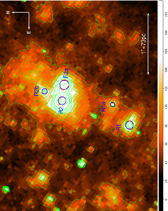
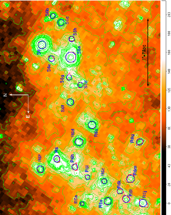
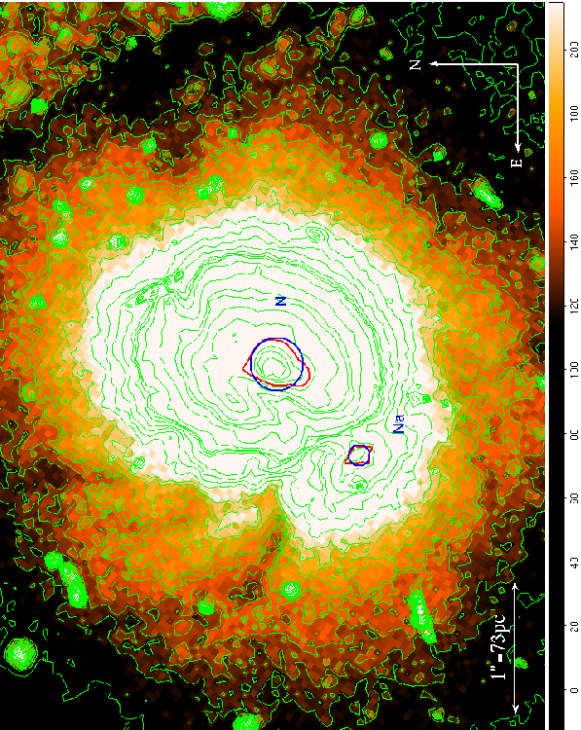
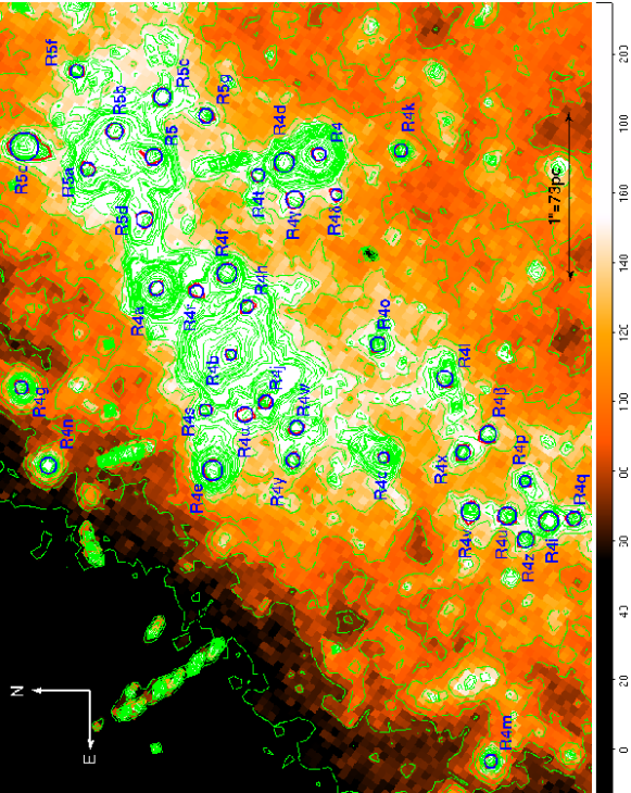
Figure 10:

Enlargements of the F606W image around the nucleus and the CNSFRs of our study with the contours overlapped. The circles correspond to the adopted radius for each region. [See the electronic edition of the Journal for a colour version of this figure where the adopted radii are in blue and the contours corresponding to the half light brightness are in red.]

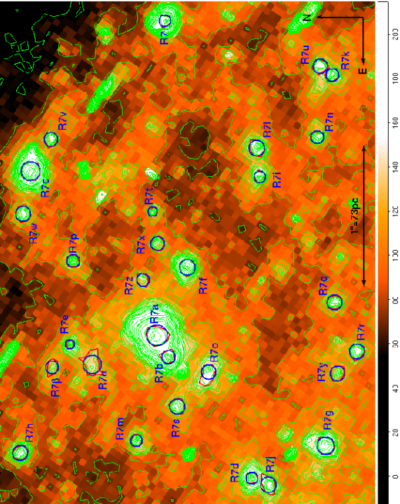
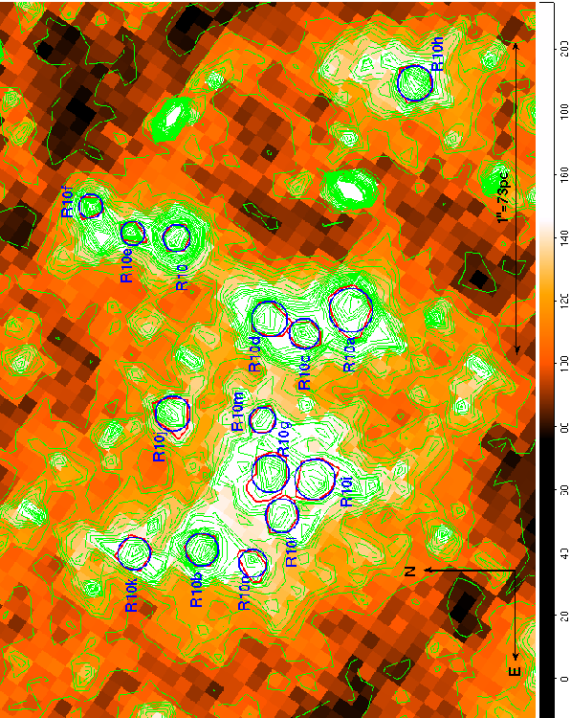
Figure 10: (cont) Enlargements of the F606W image around the CNSFRs of our study with the contours overlapped. The circles correspond to the adopted radius for each region. [See the electronic edition of the Journal for a colour version of this figure where the adopted radii are in blue and the contours corresponding to the half light brightness are in red.]

We have fitted circular regions to the intensity contours corresponding to the half light brightness distribution of each single structure (see Fig. 10), following the procedure given in Meurer et al. (1995), assuming that the regions have a circularly symmetric Gaussian profile. The radii of the single knots vary between 2.2 and 6.2 pc. Table 4 gives, for each identified knot, the position, as given by the astrometric calibration of the HST image; the radius of the circular region defined as described above together with its error; and the peak intensity in counts, as measured from the WFPC2 image. For the nucleus of NGC 3310 we measure a radius of 14.2 pc.

Table 4: Positions, radii and peak intensities derived from the HST-F606W image.

Region	position		R	I		Region	position		R	I
	$\alpha_{J2000.0}$	$\delta_{J2000.0}$	(pc)	(counts)			$\alpha_{J2000.0}$	$\delta_{J2000.0}$	(pc)	(counts)
R1	10h38m47$\aas@@fstack{s}$070	+53∘30′14$\aas@@fstack{\prime\prime}$46	4.6$\pm$0.3	322		S6	10h38m45$\aas@@fstack{s}$748	+53∘30′18$\aas@@fstack{\prime\prime}$42	4.2$\pm$0.2	544
R1a	10h38m47$\aas@@fstack{s}$032	+53∘30′14$\aas@@fstack{\prime\prime}$74	2.6$\pm$0.2	179		S6a	10h38m45$\aas@@fstack{s}$768	+53∘30′18$\aas@@fstack{\prime\prime}$00	5.5$\pm$0.2	385
R2	10h38m47$\aas@@fstack{s}$026	+53∘30′15$\aas@@fstack{\prime\prime}$55	4.7$\pm$0.2	1271		S6b	10h38m45$\aas@@fstack{s}$700	+53∘30′18$\aas@@fstack{\prime\prime}$26	2.6$\pm$0.3	237
R2a	10h38m46$\aas@@fstack{s}$997	+53∘30′15$\aas@@fstack{\prime\prime}$52	5.5$\pm$0.5	515		S6c	10h38m45$\aas@@fstack{s}$711	+53∘30′18$\aas@@fstack{\prime\prime}$14	3.4$\pm$0.3	204
R2b	10h38m47$\aas@@fstack{s}$008	+53∘30′15$\aas@@fstack{\prime\prime}$84	3.3$\pm$0.2	287		S6d	10h38m45$\aas@@fstack{s}$813	+53∘30′17$\aas@@fstack{\prime\prime}$86	2.7$\pm$0.3	180
R4	10h38m46$\aas@@fstack{s}$109	+53∘30′16$\aas@@fstack{\prime\prime}$04	2.9$\pm$0.2	2409		S6e	10h38m45$\aas@@fstack{s}$770	+53∘30′18$\aas@@fstack{\prime\prime}$28	3.0$\pm$0.2	174
R4a	10h38m46$\aas@@fstack{s}$198	+53∘30′17$\aas@@fstack{\prime\prime}$01	3.1$\pm$0.2	1942		S6f	10h38m45$\aas@@fstack{s}$842	+53∘30′18$\aas@@fstack{\prime\prime}$00	3.6$\pm$0.2	173
R4b	10h38m46$\aas@@fstack{s}$242	+53∘30′16$\aas@@fstack{\prime\prime}$57	2.5$\pm$0.2	1038		S6g	10h38m45$\aas@@fstack{s}$801	+53∘30′18$\aas@@fstack{\prime\prime}$02	2.9$\pm$0.3	172
R4c	10h38m46$\aas@@fstack{s}$311	+53∘30′15$\aas@@fstack{\prime\prime}$66	2.4$\pm$0.2	584		S6h	10h38m45$\aas@@fstack{s}$738	+53∘30′17$\aas@@fstack{\prime\prime}$98	2.8$\pm$0.3	166
R4d	10h38m46$\aas@@fstack{s}$115	+53∘30′16$\aas@@fstack{\prime\prime}$25	4.1$\pm$0.2	494		R7	10h38m45$\aas@@fstack{s}$270	+53∘30′18$\aas@@fstack{\prime\prime}$18	3.1$\pm$0.2	639
R4e	10h38m46$\aas@@fstack{s}$319	+53∘30′16$\aas@@fstack{\prime\prime}$67	4.2$\pm$0.3	489		R7a	10h38m45$\aas@@fstack{s}$520	+53∘30′18$\aas@@fstack{\prime\prime}$24	5.3$\pm$0.2	599
R4f	10h38m46$\aas@@fstack{s}$188	+53∘30′16$\aas@@fstack{\prime\prime}$59	4.2$\pm$0.2	403		R7b	10h38m45$\aas@@fstack{s}$537	+53∘30′18$\aas@@fstack{\prime\prime}$16	3.5$\pm$0.3	449
R4g	10h38m46$\aas@@fstack{s}$264	+53∘30′17$\aas@@fstack{\prime\prime}$81	2.9$\pm$0.2	391		R7c	10h38m45$\aas@@fstack{s}$390	+53∘30′19$\aas@@fstack{\prime\prime}$14	4.8$\pm$0.2	390
R4h	10h38m46$\aas@@fstack{s}$210	+53∘30′16$\aas@@fstack{\prime\prime}$47	2.8$\pm$0.4	336		R7d	10h38m45$\aas@@fstack{s}$633	+53∘30′17$\aas@@fstack{\prime\prime}$57	3.0$\pm$0.2	275
R4i	10h38m46$\aas@@fstack{s}$353	+53∘30′14$\aas@@fstack{\prime\prime}$68	4.2$\pm$0.2	304		R7e	10h38m45$\aas@@fstack{s}$527	+53∘30′18$\aas@@fstack{\prime\prime}$86	2.4$\pm$0.3	273
R4j	10h38m46$\aas@@fstack{s}$274	+53∘30′16$\aas@@fstack{\prime\prime}$36	3.0$\pm$0.3	284		R7f	10h38m45$\aas@@fstack{s}$466	+53∘30′18$\aas@@fstack{\prime\prime}$03	3.9$\pm$0.2	264
R4k	10h38m46$\aas@@fstack{s}$107	+53∘30′15$\aas@@fstack{\prime\prime}$56	2.7$\pm$0.2	271		R7g	10h38m45$\aas@@fstack{s}$607	+53∘30′17$\aas@@fstack{\prime\prime}$05	4.5$\pm$0.2	231
R4l	10h38m46$\aas@@fstack{s}$258	+53∘30′15$\aas@@fstack{\prime\prime}$30	3.4$\pm$0.5	268		R7h	10h38m45$\aas@@fstack{s}$613	+53∘30′19$\aas@@fstack{\prime\prime}$21	3.9$\pm$0.2	209
R4m	10h38m46$\aas@@fstack{s}$513	+53∘30′15$\aas@@fstack{\prime\prime}$02	2.8$\pm$0.3	259		R7i	10h38m45$\aas@@fstack{s}$394	+53∘30′17$\aas@@fstack{\prime\prime}$51	3.0$\pm$0.2	201
R4n	10h38m46$\aas@@fstack{s}$316	+53∘30′17$\aas@@fstack{\prime\prime}$66	3.4$\pm$0.3	250		R7j	10h38m45$\aas@@fstack{s}$638	+53∘30′17$\aas@@fstack{\prime\prime}$45	4.0$\pm$0.5	200
R4o	10h38m46$\aas@@fstack{s}$236	+53∘30′15$\aas@@fstack{\prime\prime}$69	3.1$\pm$0.2	241		R7k	10h38m45$\aas@@fstack{s}$313	+53∘30′17$\aas@@fstack{\prime\prime}$00	3.4$\pm$0.3	198
R4p	10h38m46$\aas@@fstack{s}$327	+53∘30′14$\aas@@fstack{\prime\prime}$82	2.4$\pm$0.2	241		R7l	10h38m45$\aas@@fstack{s}$371	+53∘30′17$\aas@@fstack{\prime\prime}$53	4.1$\pm$0.3	191
R4q	10h38m46$\aas@@fstack{s}$352	+53∘30′14$\aas@@fstack{\prime\prime}$53	3.1$\pm$0.4	227		R7m	10h38m45$\aas@@fstack{s}$603	+53∘30′18$\aas@@fstack{\prime\prime}$39	3.0$\pm$0.3	190
R4r	10h38m46$\aas@@fstack{s}$200	+53∘30′16$\aas@@fstack{\prime\prime}$77	3.1$\pm$0.3	216		R7n	10h38m45$\aas@@fstack{s}$363	+53∘30′17$\aas@@fstack{\prime\prime}$10	3.4$\pm$0.3	180
R4s	10h38m46$\aas@@fstack{s}$279	+53∘30′16$\aas@@fstack{\prime\prime}$72	2.7$\pm$0.3	212		R7o	10h38m45$\aas@@fstack{s}$549	+53∘30′17$\aas@@fstack{\prime\prime}$87	3.9$\pm$0.5	179
R4t	10h38m46$\aas@@fstack{s}$123	+53∘30′16$\aas@@fstack{\prime\prime}$40	2.9$\pm$0.4	206		R7p	10h38m45$\aas@@fstack{s}$461	+53∘30′18$\aas@@fstack{\prime\prime}$84	3.2$\pm$0.2	177
R4u	10h38m46$\aas@@fstack{s}$350	+53∘30′14$\aas@@fstack{\prime\prime}$93	3.8$\pm$0.4	206		R7q	10h38m45$\aas@@fstack{s}$494	+53∘30′16$\aas@@fstack{\prime\prime}$98	3.8$\pm$0.3	170
R4v	10h38m46$\aas@@fstack{s}$347	+53∘30′15$\aas@@fstack{\prime\prime}$14	4.0$\pm$0.4	205		R7r	10h38m45$\aas@@fstack{s}$533	+53∘30′16$\aas@@fstack{\prime\prime}$82	3.9$\pm$0.3	168
R4w	10h38m46$\aas@@fstack{s}$291	+53∘30′16$\aas@@fstack{\prime\prime}$18	2.9$\pm$0.4	204		R7s	10h38m45$\aas@@fstack{s}$576	+53∘30′18$\aas@@fstack{\prime\prime}$10	4.0$\pm$0.2	165
R4x	10h38m46$\aas@@fstack{s}$308	+53∘30′15$\aas@@fstack{\prime\prime}$19	3.1$\pm$0.3	201		R7t	10h38m45$\aas@@fstack{s}$422	+53∘30′18$\aas@@fstack{\prime\prime}$27	2.4$\pm$0.3	162
R4y	10h38m46$\aas@@fstack{s}$313	+53∘30′16$\aas@@fstack{\prime\prime}$20	2.9$\pm$0.4	194		R7u	10h38m45$\aas@@fstack{s}$306	+53∘30′17$\aas@@fstack{\prime\prime}$08	3.7$\pm$0.4	160
R4z	10h38m46$\aas@@fstack{s}$366	+53∘30′14$\aas@@fstack{\prime\prime}$81	3.5$\pm$0.3	191		R7v	10h38m45$\aas@@fstack{s}$364	+53∘30′18$\aas@@fstack{\prime\prime}$99	3.7$\pm$0.3	157
R4$\alpha$	10h38m46$\aas@@fstack{s}$282	+53∘30′16$\aas@@fstack{\prime\prime}$48	3.3$\pm$0.4	187		R7w	10h38m45$\aas@@fstack{s}$423	+53∘30′19$\aas@@fstack{\prime\prime}$19	3.9$\pm$0.2	154
R4$\beta$	10h38m46$\aas@@fstack{s}$296	+53∘30′15$\aas@@fstack{\prime\prime}$04	3.7$\pm$0.3	183		R7x	10h38m45$\aas@@fstack{s}$447	+53∘30′18$\aas@@fstack{\prime\prime}$24	3.5$\pm$0.2	152
R4$\gamma$	10h38m46$\aas@@fstack{s}$140	+53∘30′16$\aas@@fstack{\prime\prime}$19	3.7$\pm$0.3	166		R7y	10h38m45$\aas@@fstack{s}$550	+53∘30′16$\aas@@fstack{\prime\prime}$96	3.9$\pm$0.3	147
R4$\delta$	10h38m46$\aas@@fstack{s}$136	+53∘30′15$\aas@@fstack{\prime\prime}$94	2.6$\pm$0.3	166		R7z	10h38m45$\aas@@fstack{s}$476	+53∘30′18$\aas@@fstack{\prime\prime}$34	3.3$\pm$0.4	145
R5	10h38m46$\aas@@fstack{s}$111	+53∘30′17$\aas@@fstack{\prime\prime}$03	3.4$\pm$0.3	606		R7$\alpha$	10h38m45$\aas@@fstack{s}$543	+53∘30′18$\aas@@fstack{\prime\prime}$70	4.7$\pm$0.6	143
R5a	10h38m46$\aas@@fstack{s}$119	+53∘30′17$\aas@@fstack{\prime\prime}$42	3.1$\pm$0.4	370		R7$\beta$	10h38m45$\aas@@fstack{s}$545	+53∘30′18$\aas@@fstack{\prime\prime}$99	3.4$\pm$0.4	138
R5b	10h38m46$\aas@@fstack{s}$094	+53∘30′17$\aas@@fstack{\prime\prime}$26	3.6$\pm$0.4	313		R10	10h38m45$\aas@@fstack{s}$309	+53∘30′08$\aas@@fstack{\prime\prime}$14	3.1$\pm$0.2	354
R5c	10h38m46$\aas@@fstack{s}$104	+53∘30′17$\aas@@fstack{\prime\prime}$79	6.2$\pm$0.6	262		R10a	10h38m45$\aas@@fstack{s}$335	+53∘30′07$\aas@@fstack{\prime\prime}$59	5.1$\pm$0.5	303
R5d	10h38m46$\aas@@fstack{s}$153	+53∘30′17$\aas@@fstack{\prime\prime}$08	3.6$\pm$0.3	244		R10b	10h38m45$\aas@@fstack{s}$420	+53∘30′08$\aas@@fstack{\prime\prime}$06	3.8$\pm$0.2	270
R5e	10h38m46$\aas@@fstack{s}$071	+53∘30′16$\aas@@fstack{\prime\prime}$97	3.7$\pm$0.2	222		R10c	10h38m45$\aas@@fstack{s}$343	+53∘30′07$\aas@@fstack{\prime\prime}$73	3.5$\pm$0.3	260
R5f	10h38m46$\aas@@fstack{s}$054	+53∘30′17$\aas@@fstack{\prime\prime}$48	3.0$\pm$0.2	206		R10d	10h38m45$\aas@@fstack{s}$338	+53∘30′07$\aas@@fstack{\prime\prime}$84	4.1$\pm$0.4	251
R5g	10h38m46$\aas@@fstack{s}$083	+53∘30′16$\aas@@fstack{\prime\prime}$71	3.2$\pm$0.3	193		R10e	10h38m45$\aas@@fstack{s}$307	+53∘30′08$\aas@@fstack{\prime\prime}$28	2.8$\pm$0.3	235
R6	10h38m45$\aas@@fstack{s}$935	+53∘30′18$\aas@@fstack{\prime\prime}$20	3.4$\pm$0.2	378		R10f	10h38m45$\aas@@fstack{s}$298	+53∘30′08$\aas@@fstack{\prime\prime}$41	2.8$\pm$0.4	222
R6a	10h38m46$\aas@@fstack{s}$009	+53∘30′17$\aas@@fstack{\prime\prime}$83	2.2$\pm$0.3	342		R10g	10h38m45$\aas@@fstack{s}$393	+53∘30′07$\aas@@fstack{\prime\prime}$84	4.4$\pm$0.6	200
R6b	10h38m45$\aas@@fstack{s}$879	+53∘30′17$\aas@@fstack{\prime\prime}$69	3.9$\pm$0.2	260		R10h	10h38m45$\aas@@fstack{s}$254	+53∘30′07$\aas@@fstack{\prime\prime}$38	4.1$\pm$0.3	199
R6c	10h38m45$\aas@@fstack{s}$972	+53∘30′17$\aas@@fstack{\prime\prime}$51	2.7$\pm$0.2	258		R10i	10h38m45$\aas@@fstack{s}$395	+53∘30′07$\aas@@fstack{\prime\prime}$70	4.7$\pm$0.5	182
R6d	10h38m45$\aas@@fstack{s}$907	+53∘30′17$\aas@@fstack{\prime\prime}$88	4.2$\pm$0.3	242		R10j	10h38m45$\aas@@fstack{s}$371	+53∘30′08$\aas@@fstack{\prime\prime}$15	4.0$\pm$0.5	177
R6e	10h38m46$\aas@@fstack{s}$005	+53∘30′17$\aas@@fstack{\prime\prime}$46	3.9$\pm$0.4	221		R10k	10h38m45$\aas@@fstack{s}$421	+53∘30′08$\aas@@fstack{\prime\prime}$27	3.8$\pm$0.3	177
R6f	10h38m45$\aas@@fstack{s}$952	+53∘30′18$\aas@@fstack{\prime\prime}$44	3.7$\pm$0.2	215		R10l	10h38m45$\aas@@fstack{s}$408	+53∘30′07$\aas@@fstack{\prime\prime}$80	3.9$\pm$0.3	173
R6g	10h38m45$\aas@@fstack{s}$907	+53∘30′16$\aas@@fstack{\prime\prime}$99	3.4$\pm$0.4	170		R10m	10h38m45$\aas@@fstack{s}$374	+53∘30′07$\aas@@fstack{\prime\prime}$86	3.1$\pm$0.3	169
R6h	10h38m45$\aas@@fstack{s}$948	+53∘30′17$\aas@@fstack{\prime\prime}$94	3.1$\pm$0.3	168		R10n	10h38m45$\aas@@fstack{s}$424	+53∘30′07$\aas@@fstack{\prime\prime}$90	3.1$\pm$0.4	168
R6i	10h38m45$\aas@@fstack{s}$965	+53∘30′17$\aas@@fstack{\prime\prime}$75	2.5$\pm$0.2	168		N	10h38m45$\aas@@fstack{s}$893	+53∘30′11$\aas@@fstack{\prime\prime}$47	14.2$\pm$1.0	3735
R6j	10h38m46$\aas@@fstack{s}$007	+53∘30′16$\aas@@fstack{\prime\prime}$94	4.0$\pm$0.5	165		Na	10h38m45$\aas@@fstack{s}$970	+53∘30′10$\aas@@fstack{\prime\prime}$85	5.8$\pm$0.6	370
R6k	10h38m45$\aas@@fstack{s}$988	+53∘30′17$\aas@@fstack{\prime\prime}$28	3.1$\pm$0.2	160
R6l	10h38m46$\aas@@fstack{s}$001	+53∘30′17$\aas@@fstack{\prime\prime}$19	3.7$\pm$0.4	156
R6m	10h38m45$\aas@@fstack{s}$967	+53∘30′17$\aas@@fstack{\prime\prime}$12	4.2$\pm$0.5	146

Upper limits to the dynamical masses (M_∗) inside the half light radius (R) for each observed knot have been estimated under the following assumptions: (i) the systems are spherically symmetric; (ii) they are gravitationally bound; and (iii) they have isotropic velocity distributions [$\sigma^{2}$(total) = 3 $\sigma_{\ast}^{2}$]. The general expression for the virial mass of a cluster is $\eta$ $\sigma_{\ast}^{2}$ R/G, where R is the effective gravitational radius and $\eta$ is a dimensionless number that takes into account departures from isotropy in the velocity distribution and the spatial mass distribution, binary fraction, mean surface density, etc. (Boily et al., 2005; Fleck et al., 2006). Following Ho & Filippenko (1996a, b), and for consistence with Paper I, Paper II and Hägele (2008), we obtain the dynamical masses inside the half-light radius using $\eta$ = 3 and adopting the half-light radius as a reasonable approximation of the effective radius. Other authors (e.g. Spitzer, 1987; Smith & Gallagher, 2001; Moll et al., 2008) assumed that the $\eta$ value is about 9.75 to obtain the total mass. On the absence of any knowledge about the tidal radius of the clusters, we adopted this conservative approach. On the derived masses, the different adopted $\eta$ values act as multiplicative factors.

It must be noted that while we can measure the size of each knot, we do not have direct access to the stellar velocity dispersion of each individual cluster, since our spectroscopic measurements encompass a wider area (1.0 $\times$ 1.9 arcsec² which corresponds approximately to 73 $\times$ 131 pc² at the adopted distance for NGC 3310) that includes the whole CNSFRs to which each group of knots belongs. The use of these wider size scale velocity dispersion measurements to estimate the mass of each knot, leads us to overestimate the mass of the individual clusters, and hence of each CNSFR. As we can not be sure that we are actually measuring their velocity dispersion, we prefer to say that our measurements of $\sigma_{\ast}$, and hence the dynamical masses, constitute upper limits. Although we are well aware of the difficulties, still we are confident that these upper limits are valid and important for comparison with the gas kinematical measurements.

The estimated dynamical masses for each knot and their corresponding errors are listed in Table 5. For the regions that have been observed in more than one slit position, we list the derived values using the two separate stellar velocity dispersions. The dynamical masses in the rows labelled “sum” have been found by adding the individual masses in a given CNSFR, as well as the galaxy nucleus, N. The fractional errors of the dynamical masses of the individual knots and of the CNSFRs are listed in column 4. As explained above, since the stellar velocity dispersion for the R1+R2 region of NGC 3310 has a large error, we do not list the errors of the dynamical masses of the individual knots or of the whole region R12sum.

Table 5: Upper limits to the dynamical masses.

Region	Slit	M∗	error(%)		Region	Slit	M∗	error(%)		Region	Slit	M∗	error(%)
R1	S2	202:	—		R4n	S2	35$\pm$7	19		R7	S2	42$\pm$9	22
R1a	S2	115:	—		R4o	S2	32$\pm$6	18		R7a	S2	71$\pm$15	21
R2	S2	208:	—		R4p	S2	25$\pm$5	19		R7b	S2	46$\pm$11	23
R2a	S2	241:	—		R4q	S2	32$\pm$7	21		R7c	S2	64$\pm$14	21
R2b	S2	144:	—		R4r	S2	31$\pm$6	19		R7d	S2	40$\pm$9	22
R12sum	S2	911:	—		R4s	S2	27$\pm$6	20		R7e	S2	32$\pm$8	24
R4	S1	26$\pm$4	17		R4t	S2	30$\pm$6	22		R7f	S2	52$\pm$11	22
R4a	S1	27$\pm$5	17		R4u	S2	39$\pm$8	20		R7g	S2	60$\pm$13	22
R4b	S1	22$\pm$4	18		R4v	S2	41$\pm$8	19		R7h	S2	51$\pm$11	22
R4c	S1	21$\pm$4	18		R4w	S2	30$\pm$6	22		R7i	S2	40$\pm$9	22
R4d	S1	36$\pm$6	16		R4x	S2	32$\pm$6	19		R7j	S2	53$\pm$13	24
R4e	S1	38$\pm$6	17		R4y	S2	30$\pm$6	22		R7k	S2	44$\pm$10	23
R4f	S1	38$\pm$6	16		R4z	S2	36$\pm$7	19		R7l	S2	54$\pm$12	22
R4g	S1	26$\pm$4	17		R4$\alpha$	S2	33$\pm$7	21		R7m	S2	40$\pm$9	23
R4h	S1	25$\pm$5	21		R4$\beta$	S2	38$\pm$7	19		R7n	S2	44$\pm$10	23
R4i	S1	37$\pm$6	16		R4$\gamma$	S2	38$\pm$7	19		R7o	S2	52$\pm$13	25
R4j	S1	27$\pm$5	19		R4$\delta$	S2	27$\pm$5	20		R7p	S2	43$\pm$9	22
R4k	S1	24$\pm$4	17		R5	S2	35$\pm$7	19		R7q	S2	50$\pm$11	22
R4l	S1	30$\pm$7	21		R5a	S2	32$\pm$7	21		R7r	S2	52$\pm$12	22
R4m	S1	25$\pm$5	19		R5b	S2	36$\pm$7	20		R7s	S2	53$\pm$12	22
R4n	S1	30$\pm$5	18		R5c	S2	63$\pm$12	19		R7t	S2	32$\pm$8	24
R4o	S1	28$\pm$5	17		R5d	S2	36$\pm$7	19		R7u	S2	48$\pm$11	24
R4p	S1	21$\pm$4	18		R5e	S2	37$\pm$7	18		R7v	S2	48$\pm$11	23
R4q	S1	28$\pm$6	20		R5f	S2	30$\pm$5	18		R7w	S2	52$\pm$11	22
R4r	S1	27$\pm$5	18		R5g	S2	33$\pm$6	19		R7x	S2	46$\pm$10	22
R4s	S1	24$\pm$5	19		R45sum	S2	1317$\pm$41	3		R7y	S2	52$\pm$12	22
R4t	S1	26$\pm$5	21		R6	S2	28$\pm$8	30		R7z	S2	44$\pm$11	24
R4u	S1	34$\pm$6	19		R6a	S2	18$\pm$6	32		R7$\alpha$	S2	63$\pm$15	25
R4v	S1	36$\pm$7	19		R6b	S2	32$\pm$9	29		R7$\beta$	S2	44$\pm$11	24
R4w	S1	26$\pm$5	21		R6c	S2	22$\pm$7	30		R7sum	S2	1413$\pm$60	4
R4x	S1	28$\pm$5	18		R6d	S2	35$\pm$10	30		R10	S1	33$\pm$5	17
R4y	S1	26$\pm$5	21		R6e	S2	32$\pm$10	31		R10a	S1	53$\pm$10	18
R4z	S1	31$\pm$6	18		R6f	S2	30$\pm$9	29		R10b	S1	40$\pm$6	16
R4$\alpha$	S1	29$\pm$6	20		R6g	S2	28$\pm$9	31		R10c	S1	37$\pm$6	18
R4$\beta$	S1	33$\pm$6	18		R6h	S2	26$\pm$8	30		R10d	S1	43$\pm$8	18
R4$\gamma$	S1	33$\pm$6	18		R6i	S2	21$\pm$6	30		R10e	S1	29$\pm$5	19
R4$\delta$	S1	23$\pm$5	19		R6j	S2	33$\pm$10	31		R10f	S1	29$\pm$6	21
R4sum	S1	886$\pm$30	3		R6k	S2	25$\pm$8	30		R10g	S1	46$\pm$9	21
R4	S2	30$\pm$5	18		R6l	S2	31$\pm$10	31		R10h	S1	43$\pm$7	17
R4a	S2	31$\pm$6	18		R6m	S2	35$\pm$11	31		R10i	S1	50$\pm$9	19
R4b	S2	25$\pm$5	19		R6sum	S2	397$\pm$33	8		R10j	S1	42$\pm$8	19
R4c	S2	25$\pm$5	19		S6	S2	28$\pm$6	23		R10k	S1	40$\pm$7	17
R4d	S2	42$\pm$7	17		S6a	S2	37$\pm$8	23		R10l	S1	40$\pm$7	17
R4e	S2	43$\pm$8	18		S6b	S2	18$\pm$5	25		R10m	S1	32$\pm$6	18
R4f	S2	43$\pm$7	17		S6c	S2	23$\pm$6	24		R10n	S1	33$\pm$7	20
R4g	S2	30$\pm$5	18		S6d	S2	18$\pm$5	25		R10sum	S1	588$\pm$28	5
R4h	S2	28$\pm$6	22		S6e	S2	20$\pm$5	23		N	S1	526$\pm$57	11
R4i	S2	42$\pm$7	17		S6f	S2	24$\pm$6	23		Na	S1	216$\pm$28	13
R4j	S2	30$\pm$6	19		S6g	S2	20$\pm$5	25		Nsum	S1	742$\pm$64	9
R4k	S2	27$\pm$5	18		S6h	S2	19$\pm$5	25
R4l	S2	35$\pm$8	22		S6sum	S2	210$\pm$17	8
R4m	S2	29$\pm$6	20
masses in 105 M⊙.

5 Ionizing star cluster properties

For each of the CNSFR the total number of ionizing photons was derived from the total observed H$\alpha$ luminosities given by Díaz et al. (2000) and Pastoriza et al. (1993), correcting for the different assumed distance. Díaz et al. (2000) and Pastoriza et al. (1993) give the already extinction corrected luminosities. Díaz et al. (2000) estimated a diameter of 2 arcsec for regions R2, R4, R6, R7 and R10, 1.4 arcsec for R1 and R5, and 3.4 for the Jumbo region. For this latter region we give the values derived using the different quantities for the luminosities given by (Díaz et al., 2000, region R19) and (Pastoriza et al., 1993, region A). For R1+R2 and R4+R5 (S2) we added their H$\alpha$ luminosities. No values are found in the literature for the H$\alpha$ luminosity of regions X and Y. Our derived values of Q(H₀) constitute lower limits since we have not taken into account the fraction of photons that may have been absorbed by dust or may have escaped the region.

Once the number of Lyman continuum photons have been calculated, the masses of the ionizing star clusters, M_ion, have been derived using the solar metallicity single burst models by García-Vargas et al. (1995) which provide the number of ionizing photons per unit mass, [$Q(H_{0})/M_{ion}$]. A Salpeter initial mass function (Salpeter, 1955, IMF) has been assumed with lower and upper mass limits of 0.8 and 120 M_⊙. In order to take into account the evolution of the Hii region, we have made use of the fact that a relation exists between the degree of evolution of the cluster, as represented by the equivalent width of the H$\beta$ emission line, and the number of Lyman continuum photons per unit solar mass (e.g.  Díaz et al., 2000). We have measured the EW(H$\beta$) from our spectra (see Table 6) following the same procedure as in Hägele et al. (2006, 2008), that is defining a pseudo-continuum to take into account the absorption from the underlying stellar population. This procedure in fact may underestimate the value of the equivalent width, since it includes the contribution to the continuum by the older stellar population (see discussions in Díaz et al. 2007 and Dors et al. 2008). The derived masses for the ionizing populations of the observed CNSFRs are given in column 6 of Table 6 and are between 1 and 7 per cent of the dynamical mass (see column 9 of the table).

Table 6: Physical parameters.

Region	c(H$\alpha$)	L(H$\alpha$)	Q(H0)	EW(H$\beta$)	Mion	N${}_{e}^{c}$	MHII	Mion/M∗
								(per cent)
R1+R2	0.23a	102.0a	74.9	28.6	13.9	100c	3.38	1.5
R4	0.23a	144.0a	106.0	32.4	17.6	100b	4.78	1.6
R4+R5	0.20a	218.0a	160.0	41.7	21.4	100b	7.24	1.1
R6	0.17a	57.3a	42.1	16.7	12.4	100c	1.90	3.5
S6	0.35b	62.5b	45.9	12.5	17.4	100b	2.07	6.6
R7	0.17a	45.5a	33.5	19.4	8.7	100c	1.51	1.0
R10	0.23a	45.5a	33.5	9.7	15.7	100c	1.51	2.4
N	0.42b	113.0b	82.9	11.0	34.9	800d	0.47	4.7
J	0.23a	573.0a	421.0	82.5	31.4	200b	9.52	—
	0.19b	236.0b	174.0	82.5	12.9	200b	3.93	—
Note. Luminosities in 1038 erg s-1, masses in 105 M⊙, ionizing photons in 1050 photon s-1 and densities in cm-3
aFrom Díaz et al. (2000).
bFrom Pastoriza et al. (1993).
cAssumed from the values given by Pastoriza et al. (1993) for the other CNSFRs of this galaxy studied by them.
dDerived from the spectrum of the nucleus of NGC 3310 plotted in Fig. 5a of Pastoriza et al. (1993) (see discussion in the text).

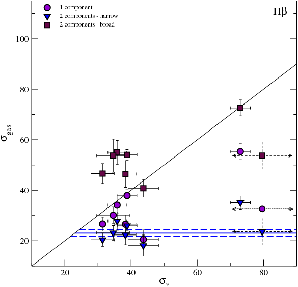
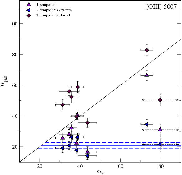
Figure 11: Upper panel: relation between velocity dispersions of the gas (derived from H$\beta$) and stars (CaT) for the CNSFRs and the nucleus of NGC 3310. Symbols are as follows: Upper panel: single Gaussian fit, violet circles; two Gaussian fit, broad component, maroon squares; narrow component, blue downward triangles; lower panel: as the upper panel for the [Oiii] line. Violet upward triangles correspond to the estimates using a single Gaussian fit, maroon diamonds represent the broad components of the two Gaussian fit and blue left triangles, the narrow components. The blue solid line represents the average velocity dispersion of the narrow component of the gas (H$\beta$ upper and [Oiii] lower panel), for the CNSFRs, and the blue dashed lines represent their estimated errors.[See the electronic edition of the Journal for a colour version of this figure.]

The amount of ionized gas (M_HII) associated to each star-forming region complex can also be derived from the H$\alpha$ luminosities using the electron density (N_e) dependency relation given by Macchetto et al. (1990) for an electron temperature of 10⁴ K. The electron density for each region (obtained from the [Sii] $\lambda\lambda$ 6717 / 6731 Å line ratio) has been taken from Pastoriza et al. (1993) for the regions in common. For the rest of the regions we assume a value of N_e equal to 100 cm^-3, the value given by Pastoriza et al. (1993) for the other CNSFRs of this galaxy studied by them. For the nucleus of NGC 3310 we find an anomalous behaviour when we estimate M_HII using the values of the density (8200 cm^-3) given by Pastoriza et al. (1993). We derive a rather low value of M_HII (5 $\times$ 10³ M_⊙) for the H$\alpha$ luminosity calculated by these authors. Then, when reviewing the density reported by Pastoriza and collaborators we found that it is consistent with the ratio of about 0.5 between the intensity values of the [Sii] $\lambda\lambda$ 6717,6731 Å emission lines given by them. However, a careful inspection of the spectrum of the nucleus of NGC 3310 plotted in Fig. 5a of Pastoriza et al. (1993) reveals that the intensities of these two [Sii] emission lines are very similar to each other (ratio of about 0.9). A rough estimate using this revised ratio yields an electron density value of about 800 cm^-3. The corresponding M_HII value derived using this lower density is an order of magnitude higher.

6 Discussion

6.1 Star and gas kinematics

Fig. 11 shows the relations between the velocity dispersions of gas and stars for NGC 3310. In the upper and lower panels we plot the relation derived from the H$\beta$ and [Oiii] emission lines, respectively. In both panels the straight line shows the one-to-one relation. In the upper panel the violet circles show the gas velocity dispersion measured from the H$\beta$ emission line using a single Gaussian fit, maroon squares and blue downward triangles show the values measured from the broad and narrow components respectively using two-component Gaussian fits. The deviant points, marked with arrows, correspond to region R1+R2, which has a spectrum with low signal-to-noise ratio for which the cross-correlation method does not provide accurate results. In the lower panel, violet upward triangles, maroon diamonds and blue left triangles correspond to the values obtained by a single Gaussian fit, and to the broad and narrow components of the two Gaussian fits, respectively. Again, the deviant points (R1+R2) are marked with arrows.

The H$\beta$ velocity dispersions of the CNSFRs of NGC 3310 derived by a single-component Gaussian fit are the same, within the errors, as the stellar ones, except for R1+R2 and R7, for which they are lower by about 50 and 25 km s^-1, respectively. For R1+R2 this can be due to an overestimate of $\sigma_{\ast}$. Given the relatively low metal abundance of NGC 3310 (Pastoriza et al., 1993) the emission lines have generally a very good signal-to-noise ratio in the spectra of the CNSFRs, while for the red continuum it depends on the particular case (see Figs. 3 and 5 for the spatial profiles and the spectra, respectively). On the other hand, the stellar velocity dispersions of the CNSFRs are lower than those of the broad component of H$\beta$ by about 20 km s^-1, again except for R1+R2 where $\sigma_{\ast}$ is greater by about 35 km s^-1, and for R7 where $\sigma_{\ast}$ and H$\beta$ broad are in good agreement. The narrow component of the CNSFRs shows velocity dispersions very similar for all the regions, with an average value of 23.0 $\pm$ 1.3 km s^-1, and is represented as a blue solid line in the upper panel of Fig. 11, while the dashed lines of the same colour represent its error.

The [Oiii] emission lines show the same behaviour as the H$\beta$ lines for the two different components. In all cases the gas narrow component has velocity dispersion lower than the stellar one, and the broad component is slightly over it. The broad component of the [Oiii] 5007 Å emission line (maroon diamonds in the figure) is wider than the stellar lines by about 20 km s^-1, except for R4+R5 (S2 slit) and R7 for which they are approximately similar. The narrow component of [Oiii] (blue left triangles in the figure) shows a relatively constant value with an average of 20.9 $\pm$ 1.8 km s^-1 (blue lines in the figure).

In general, the broad and narrow components of the H$\beta$ line have comparable fluxes. The ratios between the fluxes in the narrow and broad components of the H$\beta$ emission line of the regions (including J, X and Y) vary from 0.95 to 1.65, except for R10 and R7 for which we find ratios of 0.65 and 2.5, respectively. The ratio of the narrow to broad [Oiii] fluxes is between 0.85 and 1.5; R10 and R7, for which this value is 0.65 and 1.98 respectively, are again the exception.

The behaviour of the velocity dispersions of the CNSFRs is found to be different in NGC 3310 from what was found for NGC 2903 and NGC 3351 (Papers I and II). For NGC 3310 we find a very good agreement in most cases between velocity dispersions derived from gaseous and stellar lines assuming a single component for the gas. For NGC 2903 and NGC 3351, in contrast, the velocity dispersions derived from emission lines measured using a single Gaussian fit are very different from the stellar ones (lower for H$\beta$ and higher for [Oiii]) by about 20 km s^-1; see discussion in Paper II). Remarkably, the velocity dispersions derived from the narrow components of the two Gaussian fits show a relatively constant value for the whole CNSFR sample (about 23 kms^-1). If this narrow component is identified with ionized gas in a rotating disc, therefore supported by rotation, then the broad component could, in principle, correspond to the gas response to the gravitational potential of the stellar cluster, supported by dynamical pressure, explaining the coincidence with the stellar velocity dispersion in most cases in the H$\beta$ line (see Pizzella et al., 2004, and references therein). The velocity excess shown by the broad component of H$\beta$ and [Oiii] in most CNSFRs of NGC 3310 could be identified with peculiar velocities in the ionized gas (mainly in the high ionization gas) related to massive star winds or even supernova remnants.

Our interpretation of the emission line structures, in the present study and in Papers I and II, parallels that of the studies of Westmoquette and collaborators (see for example Westmoquette et al. 2007a,b). They observed a narrow ($\sim$ 35-100 km s^-1) and a broad ($\sim$ 100-400 km s^-1) component to the H$\alpha$ line across their four fields in the dwarf galaxy NGC 1569. They conclude that “the most likely explanation of the narrow component is that it represents the general disturbed optically emitting ionized interstellar medium (ISM), arising through a convolution of the stirring effects of the starburst and gravitational virial motions”. They also conclude that “the broad component results from the highly turbulent velocity field associated with the interaction of the hot phase of the ISM (material that is photo-evaporated or thermally evaporated through the action of the strong ambient radiation field, or mechanically ablated by the impact of fast-flowing cluster winds) with cooler gas knots, setting up turbulent mixing layers (e.g. Begelman & Fabian, 1990; Slavin et al., 1993)”. However, our broad component velocity dispersion values derived from H$\beta$, all significantly lower than 100 km s^-1 and similar to the stellar velocity dispersions, resemble more their narrow component values. This is the same behaviour that we find in the broad component of the [Oiii] emission line for the CNSFRs of NGC 3310. The [Oiii] line profiles of the regions in Papers I and II on the other hand, behave as those described by Westmoquette and collaborators.

There are other studies that identified an underlying broad component to the recombination emission lines such as Díaz et al. (1987); Terlevich et al. (1996) in the M33 giant Hii region NGC 604; Chu & Kennicutt Jr. (1994); Melnick, Tenorio-Tagle & Terlevich (1999) in the central region of 30 Doradus; Mendez & Esteban (1997) in four Wolf-Rayet galaxies, and Homeier & Gallagher (1999) in the starburst galaxy NGC 7673. More recently, Westmoquette et al. (2007c, 2009) found a broad feature in the H$\alpha$ emission lines in the starburst core of M82; Östlin et al. (2007) and James et al. (2009) in the blue compact galaxies ESO 338-IG04 and Mrk 996, respectively; Sidoli et al. (2006); Firpo et al. (2009) in giant extragalactic Hii regions, and Hägele (2008) in CNSFRs of early type spiral galaxies. The first two and the last three studies also found this broad component in the forbidden emission lines.

In the nuclear region of the galaxy the stars and the broad component of the ionized gas, both for H$\beta$ and [Oiii] have the same width, with a $\sigma$ of about 73 and 83 km s^-1, respectively. The profiles of the nuclear lines hence, behave similarly to what is described by Westmoquette and collaborators. The gas narrow component however shows a substantially lower velocity dispersion though still higher by about 15 km s^-1, than that of the CNSFRs.

For regions J, X and Y we can not derive a stellar velocity dispersion due to the low signal-to-noise ratio of their continuum and the noise added by subtracting the large amount of emission lines present in their red spectra (see right panels of Fig. 5). However, if we analyze the velocity dispersions derived from their strong emission lines in the blue spectral range we find values very similar to those of the other CNSFRs (see Table 2).

Fig. 12 presents the radial velocities derived from the H$\beta$ and [Oiii] emission lines and the CaT absorptions along the slit for each angular slit position of NGC 3310, S1 in the upper panel and S2 in the lower one. The rotation curves seem to have the turnover points located in or near the star-forming ring. Due to the relatively low metallicity of NGC 3310 (Pastoriza et al., 1993), the gas emission lines are very strong in the central zone of the galaxy and we can derive the radial velocity of the gas much further (up to 18 ″) than for the stellar CaT absorptions. The gas H$\beta$ and [Oiii] 5007 Å radial velocities and the stellar ones are in very good agreement, except in the zone located around R4, where we find a difference between gas and stars of about 30 to 40 km s^-1. These differences could be due to a low signal-to-noise ratio of the stellar continuum emission in this zone of the galaxy.

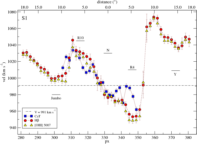
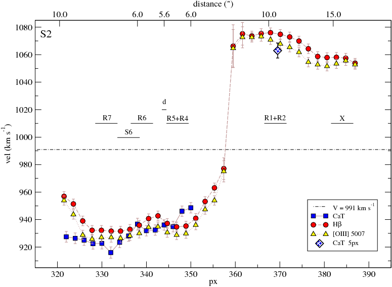
Figure 12: Radial velocities along the slit versus pixel number for each slit position of NGC 3310 (upper panel: S1; lower panel: S2) as derived from the gas emission lines (red circles: H$\beta$; upward triangles: [Oiii]) and the stellar absorption ones (blue squares). The criss-crossed white-blue diamond in the lower panel correspond to the stellar velocity of R1+R2 derived using the 5 px aperture. The individual CNSFRs and the nucleus, “N”, or the closest position to it, “d”, are marked in the plots. The dashed-dotted line is the velocity of the nucleus of NGC 3310 derived by van der Kruit (1976). The distance in arcsec from the nucleus is displayed in the upper x-axis of each panel. [See the electronic edition of the Journal for a colour version of this figure.]

In both slit positions we can appreciate a very steep slope in the radial velocity curve as measured from H$\beta$ and [Oiii], in very good agreement with each other. These strong gradients occur more or less at the same distance from the nucleus ($\sim$8 ″) towards the north-east of the galaxy, almost at the position where the two slits intersect (see Figs. 1 and 2). The curves show a step in the radial velocity of about 70 and 90 km s^-1 for S1 and S2, respectively. In Fig. 2 we indicate with two circles of 8 and 18″ radii the approximate position where this step is located and the distance from the nucleus up to where we can derive the radial velocities for S1. The stellar radial velocity of R1+R2 derived using the 5 px aperture (criss-crossed white-blue diamond in the lower panel of Fig. 12) is in very good agreement with the values derived from the gas emission lines.

A very similar result was found by Pastorini et al. (2007) using high spatial resolution spectra ($\sim$ 0.07 ″ px^-1) and moderate spectral resolution (R = $\Delta\lambda$/$\lambda$ $\sim$ 6000, yielding a resolution of $\Delta\lambda$ $\sim$ 1.108 Å px^-1 at H$\alpha$) from the Space Telescope Imaging Spectrograph (STIS) on board the HST, and using a 2 $\times$ 2 on-chip binning for the non nuclear spectra. The position angle of their slits is 170^∘ and three parallel positions were used, one of them passing across the nucleus and the other two with 0.2 ″ offset to both sides . As pointed out by Pastorini and collaborators, NGC 3310 shows a typical rotation curve expected for a rotating disc (a typical $S$ feature, Marconi et al., 2006) but the curve is disturbed. Besides, we can appreciate that near the Jumbo region there is a deviation from circular rotation motion. The step in the radial velocity found by us is an effect of the spatial resolution. In Fig. 3 of Pastorini et al. (2007), the better spatial resolution of STIS-HST resolves the steep gradient and completes the information missing in our data. This disturbed behaviour of the rotation curve of the gas in the galactic disc, characterized by non-circular motions, was also found by Mulder et al. (1995) using Hi radio data; Mulder & van Driel (1996) from Hi and Hii radio data and Kregel & Sancisi (2001) using optical data. They found a strong streaming along the spiral arms, supporting the hypothesis of a recent collision with a dwarf galaxy that triggered the circumnuclear star formation during the last 10⁸ yr. Besides, van der Kruit (1976) shows that the rotation centre of the gas is offset with respect to the stellar continuum (by $\sim$ 1.5 ″). The central velocity of NGC 3310 derived by us is in very good agreement with that previously estimated by van der Kruit (1976); Mulder et al. (1995); Mulder & van Driel (1996); Haynes et al. (1998); Kregel & Sancisi (2001). The velocity distribution is also in very good agreement with that expected for this type of galaxies (Binney & Tremaine, 1987).

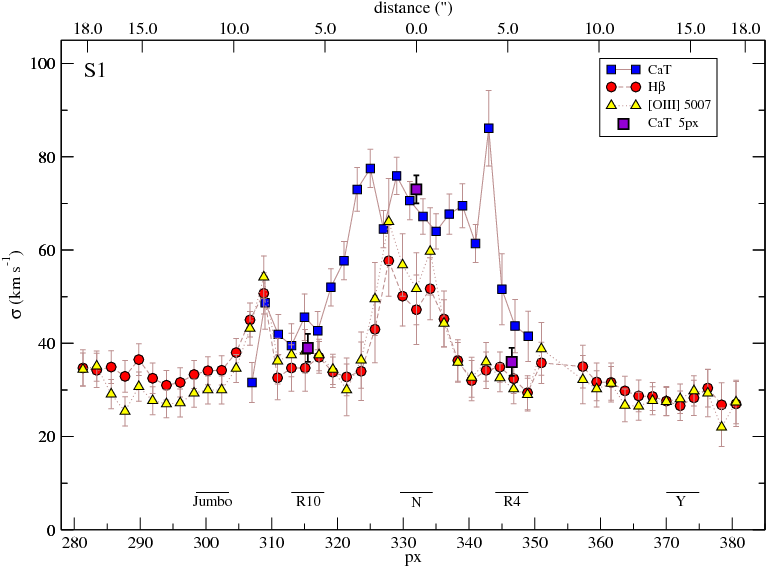
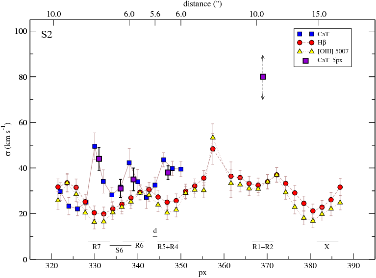
Figure 13: Velocity dispersions along the slit versus pixel number for each slit position of NGC 3310 (upper panel: S1; lower panel: S2) as derived from the gas emission lines (small red circles: H$\beta$; small yellow triangles: [Oiii]) and the stellar absorption ones (small blue squares). The stellar velocity dispersions derived for each region and the nucleus using the 5 px aperture are also plotted with violet squares. The individual CNSFRs and the nucleus, “N”, or the closest position to it, “d”, are marked in the plots. The distance in arcsec from the nucleus is displayed in the upper x-axis of each panel. [See the electronic edition of the Journal for a colour version of this figure.]

Fig. 13 shows the run of velocity dispersion along the slit versus pixel number for slit positions S1 and S2 respectively. These velocity dispersions have been derived from the gaseous emission lines, H$\beta$ and [Oiii], and the stellar absorption ones using 2 and 3 px apertures for S1 and S2, respectively. We have marked the location of the studied CNSFR and the galaxy nucleus. We have also plotted the stellar velocity dispersion derived for each region and the nucleus using 5 px apertures. The values derived with wider apertures are approximately the average of the velocity dispersions estimated using the narrower ones. Therefore, the apparent increase of the velocity dispersions of the regions lying on relatively steep parts of the rotation curve by spatial “beam smearing” of the rotational velocity gradient due to the finite angular resolution of the spectra is not so critical for the studied CNSFRs. This is due to the fact that the turnover points of the rotation curves and the star-forming ring seem to be located at the same positions, as was pointed out above. The velocity dispersions, both for stars and gas, show a behaviour characteristic of a regular circular motion in a rotating disc, a smooth plateau and a central peak. A similar result was found by Pastorini et al. (2007).

6.2 Star cluster masses

The eight CNSFRs observed in NGC 3310 show a complex structure at the HST resolution (Fig. 10), with a good number of subclusters with linear diameters between 2.2 and 6.2 pc. For these individual clusters, except for R1+R2, the derived upper limits to the masses are in the range between 1.8 and 7.1 $\times$ 10⁶ M_⊙ (see table 5), with fractional errors between $\sim$ 16 and $\sim$ 32 per cent. The upper limits to the dynamical masses estimated for the whole CNSFRs (“sum”), except for R1+R2, are between 2.1 $\times$ 10⁷ and 1.4 $\times$ 10⁸ M_⊙, with fractional errors between $\sim$3 and $\sim$8 per cent. The stellar velocity dispersion of region R1+R2 has a large associated error, so we do not quote an explicit error for its derived mass which we consider highly uncertain. The masses for the individual clusters of this CNSFR, derived using this value of the velocity dispersion are larger, between 1.2 and 2.4 $\times$ 10⁷ M_⊙. However, if we assume that the relation between the gas and the stellar velocity dispersions follows a behaviour similar to that shown by the rest of the CNSFRs of NGC 3310 (see Fig. 11) these masses could be reduced by a factor of 2.3, yielding individual masses between 5.2 $\times$ 10⁶ and 1.0 $\times$ 10⁷ M_⊙. In the same way, the total dynamical mass of R1+R2, 9.1 $\times$ 10⁸ M_⊙, would be reduced to 4.0 $\times$ 10⁸ M_⊙. The upper limits to the dynamical mass derived for the nuclear region inside the inner 14.2 pc is 5.3 $\times$ 10⁷ M_⊙, with a fractional error of about 11 per cent. This value is somewhat higher than that derived by Pastorini et al. (2007) under the assumption of the presence of a super massive black hole (SMBH) in the centre of the galaxy. When they allow for the disc inclination, this mass varies in the range 5.0 $\times$ 10⁶ - 4.2 $\times$ 10⁷ M_⊙.

The masses of the ionizing stellar clusters of the CNSFRs, derived from their H$\alpha$ luminosities (under the assumption that the regions are ionization bound and without taking into account any photon absorption by dust), are between 8.7 $\times$ 10⁵ and 2.1 $\times$ 10⁶ M_⊙ for the star-forming regions, and 3.5 $\times$ 10⁶ M_⊙ for the nucleus (see Table 6). In the case of the Jumbo region this mass vary between 1.3 and 3.1 $\times$ 10⁶ M_⊙ whether we take the H$\alpha$ luminosities from Pastoriza et al. (1993) or Díaz et al. (2000) respectively, probably because the estimated reddening constants in these two works are different (see Table 6). These different values of the luminosities can be due to the very complex structure of the region (see Fig. 1 of both works) and to different selection of the zone used to measure the H$\alpha$ fluxes. Besides, Pastoriza and colleagues used spectroscopic data while Díaz and collaborators used photometric images. In column 9 of Table 6 we show a comparison (in percentage) between the ionizing stellar masses of the circumnuclear regions and their dynamical masses. These values are approximately between 1 - 7 per cent for the CNSFRs, and 5 per cent for the nucleus of NGC 3310.

Finally, the masses of the ionized gas, also derived from their H$\alpha$ luminosities, range between 1.5 and 7.2 $\times$ 10⁵ M_⊙ for the CNSFRs, and 4.7 $\times$ 10⁴ M_⊙ for the nucleus (see Table 6). They make up a small fraction of the total mass of the regions. As in the case of the masses of the ionizing stellar clusters of the Jumbo region and for the same reasons, the mass of the ionized gas derived using the H$\alpha$ luminosities from Pastoriza et al. (1993) or from Díaz et al. (2000) are different, 3.93 and 9.52 $\times$ 10⁵ M_⊙, respectively. It should be taken into account that we have derived both the masses of the ionizing stellar clusters and of the ionized gas from the H$\alpha$ luminosity of the CNSFRs assuming that they consist of one single component. However, if we consider only the broad component whose kinematics follows that of the stars in the regions, all derived quantities would be smaller by a factor of 2.

Comparing the colours of the small-scale clusters from HST data with models, Elmegreen et al. (2002) suggest that most of these clusters contain masses from 10⁴ M_⊙ to several times 10⁴ M_⊙. For the large-scale “hot-spots” they estimate masses ranging from 10⁴ to several times 10⁵ M_⊙. For their 108+109 region (almost equivalent to the Jumbo region) they derived a mass of 6.3 $\times$ $10^{5}$ M_⊙, similar to the value derived by Pastoriza et al. (1993), 7 $\times$ $10^{5}$ M_⊙. They estimated from the unusually large H and Heii emission line luminosities, that this region must contain 220 WN and 570 OB stars. Regarding other regions, Elmegreen and colaborators derived a mass of $10^{6}$ M_⊙ for their region 78 using the NIR data and 7.7 $\times$ $10^{6}$ M_⊙ from their optical ones. Besides, they found 17 candidate SSCs, with masses in the range 2 $\times$ $10^{4}$ to 4.5 $\times$ $10^{5}$ M_⊙. Some of them coincide with the CNSFRs studied by us, such as 48, 49 and 50, approximately coincident with R5 and R6. These SSCs are mostly in the innermost southern spiral arm, with some in the northern one or outside the southern arm of the ring (Elmegreen et al., 2002). Their derived (J-H) colours suggest two different populations of SSCs, a very young of few million years and an older one in a range between 10 and 50 million years, with the younger clusters located in the northern part of the ring.

It should be recalled that we have estimated the dynamical masses through the virial theorem under the assumption that the systems are spherically symmetric, gravitationally bound and have isotropic velocity distribution. We have used the stellar velocity dispersions derived from the CaT absorptions features and the cluster sizes measured from the high spatial resolution WFPC2-PC1 HST image. As mentioned at the end of section 4, the use of these wider size scale velocity dispersion measurements to estimate the mass of each knot, can lead to an overestimate of the mass of the individual clusters, and hence of each CNSFR (see Paper I).

However, as can be seen in the HST-NICMOS images (right-hand panel of Fig. 1), the CNSFRs are clearly visible in the IR and dominate the light inside the apertures observed (see Elmegreen et al., 2002, for a detailed analysis of the IR images). All the regions analyzed show up very prominently in the near-IR and therefore we can assume that the light at the CaT wavelength region is dominated by the stars in the clusters. The IR CaT is very strong, in fact the strongest stellar feature, in young clusters older than 4 Myr Terlevich et al. (1990). Besides, we detect a minimum in the velocity dispersion at the position of most of the clusters, indicating that they are kinematically distinct. We can not be sure though that we are actually measuring their velocity dispersion and thus prefer to say that our measurements of $\sigma_{\ast}$ and hence the dynamical masses constitute upper limits. Although we are well aware of the difficulties, still we are confident that these upper limits are valid and important for comparison with the gas kinematic measurements.

Another important fact that can affect the estimated dynamical masses is the presence of binaries among the red supergiant and red giant populations from which we have derived the stellar velocity dispersions. In a recent work, Bosch et al. (2009) using the Gemini Multi-Object Spectrograph (GEMINI-GMOS) data, have investigated the presence of binary stars within the ionizing cluster of 30 Doradus. From a seven epoch observing campaign they have detected a rate of binary system candidates within their OB star sample of $\sim$ 50 %. Interestingly enough, this detection rate is consistent with a spectroscopic population of 100 % binaries, when the observational parameters described in the simulations by Bosch & Meza (2001) are set for their observations. From their final sample of ‘single’ stars they estimated a radial velocity dispersion of 8.3 km s^-1. When they derived $\sigma_{\ast}$ from a single epoch, they found values as high as 30 km s^-1, consistent with the values derived from single epoch NTT observations by Bosch et al. (2001).

Although the environment of our CNSFRs is very different from that of 30 Dor and the stellar components of the binary systems studied by Bosch et al. (2009) are very different from the stars present in our regions from where the CaT arise (red supergiants), this is an illustrative observational example of the problem. The orbital motions of the stars in binary (multiple) systems produce an overestimate of the velocity dispersions and hence of the dynamical masses. The single-star assumption introduces a systematic error that depends on the properties of the star cluster and the binary population, with an important effect on the cluster mass if the typical orbital velocity of a binary component is of the order of, or larger than, the velocity dispersion of the single/binary stars in the potential of the cluster (Kouwenhoven & de Grijs, 2008). As was pointed out by these authors, the relative weights between the single and binary stars in the velocity dispersion measurements depend on the binary fraction, which, together with the semi-major axis or period distribution, are the most important parameters in order to determine if the binary population affects the estimated dynamical masses. Their simulations indicate that the dynamical mass is overestimated by 70 %, 50 % and 5 % for a measured stellar velocity dispersion in the line of sight of 1 km s^-1, 2 km s^-1 and 10 km s^-1 respectively. They therefore conclude that most of the known dynamical masses of massive star clusters are only mildly affected by the presence of binaries. Hence, although the binary fraction of the red supergiants and red giants in our circumnuclear regions is unknown, since the smallest estimated velocity dispersion is 31 km s^-1, we can assume that the contribution of binaries to the stellar velocity dispersions is not important.

7 Summary and conclusions

We have measured gas and stellar velocity dispersions in eight CNSFRs and the nucleus of the barred spiral galaxy NGC 3310. The stellar velocity dispersions have been measured from the CaT lines at $\lambda\lambda$ 8494, 8542, 8662 Å, while the gas velocity dispersions have been measured by Gaussian fits to the H$\beta$ $\lambda$ 4861 Å and the [Oiii] $\lambda$ 5007Å emission lines on high dispersion spectra.

Stellar velocity dispersions are between 31 and 73 km s^-1. The stellar and gas velocity dispersion are in relatively good agreement, with the former being slightly larger. The velocity dispersions from [Oiii] 5007 Å behave similarly to those from H$\beta$. However, the best Gaussian fits involve two different components for the gas: a “broad component” with a velocity dispersion larger than that measured for the stars by about 20 km s^-1, and a “narrow component” with a velocity dispersion lower than the stellar one by about 30 km s^-1. This last velocity component shows a relatively constant value for the two gas emission lines, close to 22 km s^-1 and also close to that measured for CNSFRs in the previously studied NGC 3351 and NGC 2903. The velocity dispersion for the broad component of H$\beta$ is similar to that of [OIII], contrary to what we found in Papers I and II for NGC 2903 and NGC 3351. We find a velocity shift between the narrow and broad components of the multi-Gaussian fits that vary between -25 and 20 km s^-1 in radial velocity.

When plotted in a [Oiii]/H$\beta$ versus [Nii]/H$\alpha$ diagnostic diagram, the broad and narrow systems and those values derived using a single Gaussian fit show very similar values, lying in the region of low-metallicity Hii-like objects. This is in contrast to what we found in Papers I and II where the two systems are clearly segregated for the high-metallicity regions of NGC 3351 and NGC 2903, with the narrow component showing lower excitation and being among the lowest excitation line ratios detected within the SDSS data set of starburst systems.

The rotation curve of NGC 3310 shows a typical $S$ feature, with the presence of some perturbations, particularly near the location of the Jumbo region. The values derived from the gas emission lines and the stellar absorption features are in very good agreement. The position going through the nucleus shows maximum and minimum values more or less coincident with the location of the CNSFRs.

The upper limits to the dynamical masses estimated from the stellar velocity dispersion using the virial theorem for the CNSFRs are in the range between 2.1 $\times\,10^{7}$ and 1.4 $\times\,10^{8}$ M_⊙. For the nuclear region inside the inner 14.2 pc this upper limit is 5.3 $\times\,10^{7}$ M_⊙. The upper limits to the derived masses for the individual clusters are between 1.8 and 7.1 $\times$ 10⁶ M_⊙.

Masses of the ionizing stellar clusters of the CNSFRs have been derived from their H$\alpha$ luminosities under the assumption that the regions are ionization bound and without taking into account any photon absorption by dust. These masses derived for the star forming complexes of NGC 3310 are between 8.7 $\times\,10^{5}$ and 2.1 $\times\,10^{6}$ M_⊙, and is 3.5 $\times\,10^{6}$ for the nucleus (see table 6). Therefore, the ratio of the ionizing stellar population to the total dynamical mass is between 0.01 and 0.07.

Derived masses for the ionized gas, also from their H$\alpha$ luminosities, vary between 1.5 and 7.2 $\times\,10^{5}$ M_⊙ for the CNSFRs. For the nucleus, the derived mass of ionized gas is 4.7 $\times\,10^{4}$ M_⊙.

It is interesting to note that, according to our findings, the SSC in CNSFRs seem to contain composite stellar populations. Although the youngest one dominates the UV light and is responsible for the gas ionization, it constitutes only about 10 per cent of the total mass. This can explain the low EWs of emission lines measured in these regions. This may well apply to studies of other SSC and therefore conclusions drawn from fits of single stellar population models should be taken with caution (e.g.  McCrady et al., 2003; Larsen et al., 2004). Furthermore, the composite nature of the CNSFRs means that star formation in the rings is a process that has taken place over time periods much longer than those implied by the properties of the ionized gas.

References

- Athanassoula (1992) Athanassoula E., 1992, Mon. Not. R. Astron. Soc., 259, 345
- Balick & Heckman (1981) Balick B., Heckman T., 1981, Astron. Astrophys., 96, 271
- Barth et al. (1995) Barth A. J., Ho L. C., Filippenko A. V., Sargent W. L., 1995, Astron. J., 110, 1009
- Bastian et al. (2005) Bastian N., Gieles M., Lamers H. J. G. L. M., Scheepmaker R. A., de Grijs R., 2005, Astron. Astrophys., 431, 905
- Bastian et al. (2006) Bastian N., Saglia R. P., Goudfrooij P., Kissler-Patig M., Maraston C., Schweizer F., Zoccali M., 2006, Astron. Astrophys., 448, 881
- Begelman & Fabian (1990) Begelman M. C., Fabian A. C., 1990, Mon. Not. R. Astron. Soc., 244, 26P
- Binney & Tremaine (1987) Binney J., Tremaine S., 1987, Galactic dynamics. Princeton, NJ, Princeton University Press, 1987, 747 p.
- Boily et al. (2005) Boily C. M., Lançon A., Deiters S., Heggie D. C., 2005, Astrophys. J. Letters, 620, L27
- Bosch & Meza (2001) Bosch G., Meza A., 2001, in Revista Mexicana de Astronomia y Astrofisica Conference Series Vol. 11, Observed and Intrinsic Properties of Binary Star Orbits. pp 29–+
- Bosch et al. (2001) Bosch G., Selman F., Melnick J., Terlevich R., 2001, Astron. Astrophys., 380, 137
- Bosch et al. (2009) Bosch G., Terlevich E., Terlevich R., 2009, Astron. J., 137, 3437
- Bresolin & Kennicutt (1997) Bresolin F., Kennicutt Jr. R. C., 1997, Astron. J., 113, 975
- Bresolin et al. (1999) Bresolin F., Kennicutt Jr. R. C., Garnett D. R., 1999, Astrophys. J., 510, 104
- Chu & Kennicutt (1994) Chu Y.-H., Kennicutt Jr. R. C., 1994, Astrophys. J., 425, 720
- Cumming et al. (2008) Cumming R. J., Fathi K., Östlin G., Marquart T., Márquez I., Masegosa J., Bergvall N., Amram P., 2008, Astron. Astrophys., 479, 725
- de Vaucouleurs et al. (1991) de Vaucouleurs G., de Vaucouleurs A., Corwin Jr. H. G., Buta R. J., Paturel G., Fouque P., 1991, Third Reference Catalogue of Bright Galaxies. Volume 1-3, XII, 2069 pp. 7 figs.. Springer-Verlag Berlin Heidelberg New York
- Díaz (1988) Díaz A. I., 1988, Mon. Not. R. Astron. Soc., 231, 57
- Díaz et al. (2000) Díaz A. I., Álvarez-Álvarez M., Terlevich E., Terlevich R., Portal M. S., Aretxaga I., 2000, Mon. Not. R. Astron. Soc., 311, 120
- Díaz et al. (2000) Díaz A. I., Castellanos M., Terlevich E., Luisa García-Vargas M., 2000, Mon. Not. R. Astron. Soc., 318, 462
- Díaz et al. (2007) Díaz A. I., Terlevich E., Castellanos M., Hägele G. F., 2007, Mon. Not. R. Astron. Soc., 382, 251
- Díaz et al. (1987) Díaz A. I., Terlevich E., Pagel B. E. J., Víilchez J. M., Edmunds M. G., 1987, Mon. Not. R. Astron. Soc., 226, 19
- Díaz et al. (1989) Díaz A. I., Terlevich E., Terlevich R., 1989, Mon. Not. R. Astron. Soc., 239, 325
- Díaz et al. (1991) Díaz A. I., Terlevich E., Vílchez J. M., Pagel B. E. J., Edmunds M. G., 1991, Mon. Not. R. Astron. Soc., 253, 245
- Dors et al. (2008) Dors Jr. O. L., Storchi-Bergmann T., Riffel R. A., Schimdt A. A., 2008, Astron. Astrophys., 482, 59
- Elmegreen et al. (2002) Elmegreen D. M., Chromey F. R., McGrath E. J., Ostenson J. M., 2002, Astron. J., 123, 1381
- Falco et al. (1999) Falco E. E., Kurtz M. J., Geller M. J., Huchra J. P., Peters J., Berlind P., Mink D. J., Tokarz S. P., Elwell B., 1999, Publ. Astron. Soc. Pac., 111, 438
- Firpo et al. (2009) Firpo V., Bosch G., Hägele G. F., Morrell N., 2009, Mon. Not. R. Astron. Soc., submitted
- Fleck et al. (2006) Fleck J.-J., Boily C. M., Lançon A., Deiters S., 2006, Mon. Not. R. Astron. Soc., 369, 1392
- García-Vargas et al. (1995) García-Vargas M. L., Bressan A., Díaz A. I., 1995, Astron. and Astrophys. Suppl. Sries, 112, 35
- González-Delgado et al. (1994) González-Delgado R. M., Pérez E., Tenorio-Tagle G., Vílchez J. M., Terlevich E., Terlevich R., Telles E., Rodríguez-Espinosa J. M., Mas-Hesse M., García-Vargas M. L., Díaz A. I., Cepa J., Castañeda H., 1994, Astrophys. J., 437, 239
- Hägele (2008) Hägele G. F., 2008, PhD thesis, Universidad Autónoma de Madrid
- Hägele et al. (2007) Hägele G. F., Díaz A. I., Cardaci M. V., Terlevich E., Terlevich R., 2007, Mon. Not. R. Astron. Soc., 378, 163 (Paper I)
- Hägele et al. (2009) Hägele G. F., Díaz A. I., Cardaci M. V., Terlevich E., Terlevich R., 2009, Mon. Not. R. Astron. Soc., 396, 2295 (Paper II)
- Hägele et al. (2008) Hägele G. F., Díaz A. I., Terlevich E., Terlevich R., Pérez-Montero E., Cardaci M. V., 2008, Mon. Not. R. Astron. Soc., 383, 209
- Hägele et al. (2006) Hägele G. F., Pérez-Montero E., Díaz A. I., Terlevich E., Terlevich R., 2006, Mon. Not. R. Astron. Soc., 372, 293
- Harper & Low (1973) Harper Jr. D. A., Low F. J., 1973, Astrophys. J. Letters, 182, L89+
- Haynes et al. (1998) Haynes M. P., van Zee L., Hogg D. E., Roberts M. S., Maddalena R. J., 1998, Astron. J., 115, 62
- Ho & Filippenko (1996a) Ho L. C., Filippenko A. V., 1996a, Astrophys. J. Letters, 466, L83+
- Ho & Filippenko (1996b) Ho L. C., Filippenko A. V., 1996b, Astrophys. J., 472, 600
- Homeier & Gallagher (1999) Homeier N. L., Gallagher J. S., 1999, Astrophys. J., 522, 199
- James et al. (2009) James B. L., Tsamis Y. G., Barlow M. J., Westmoquette M. S., Walsh J. R., Cuisinier F., Exter K. M., 2009, ArXiv e-prints
- Jiménez-Benito et al. (2000) Jiménez-Benito L., Díaz A. I., Terlevich R., Terlevich E., 2000, Mon. Not. R. Astron. Soc., 317, 907
- Kennicutt (1998a) Kennicutt Jr. R. C., 1998a, Ann. Rev. Astron. Astrophys., 36, 189
- Kennicutt (1998b) Kennicutt Jr. R. C., 1998b, Astrophys. J., 498, 541
- Kennicutt et al. (1989) Kennicutt Jr. R. C., Keel W. C., Blaha C. A., 1989, Astron. J., 97, 1022
- Kouwenhoven & de Grijs (2008) Kouwenhoven M. B. N., de Grijs R., 2008, Astron. Astrophys., 480, 103
- Kregel & Sancisi (2001) Kregel M., Sancisi R., 2001, Astron. Astrophys., 376, 59
- Kurtz & Mink (1998) Kurtz M. J., Mink D. J., 1998, Publ. Astron. Soc. Pac., 110, 934
- Larsen et al. (2001) Larsen S. S., Brodie J. P., Elmegreen B. G., Efremov Y. N., Hodge P. W., Richtler T., 2001, Astrophys. J., 556, 801
- Larsen et al. (2004) Larsen S. S., Brodie J. P., Hunter D. A., 2004, Astron. J., 128, 2295
- Leitherer et al. (1999) Leitherer C., Schaerer D., Goldader J. D., Delgado R. M. G., Robert C., Kune D. F., de Mello D. F., Devost D., Heckman T. M., 1999, Astrophys. J., Suppl. Ser., 123, 3
- Macchetto et al. (1990) Macchetto F., Colina L., Golombek D., Perryman M. A. C., di Serego Alighieri S., 1990, Astrophys. J., 356, 389
- Maoz et al. (1996) Maoz D., Barth A. J., Sternberg A., Filippenko A. V., Ho L. C., Macchetto F. D., Rix H.-W., Schneider D. P., 1996, Astron. J., 111, 2248
- Marconi et al. (2006) Marconi A., Pastorini G., Pacini F., Axon D. J., Capetti A., Macchetto D., Koekemoer A. M., Schreier E. J., 2006, Astron. Astrophys., 448, 921
- McCrady et al. (2003) McCrady N., Gilbert A. M., Graham J. R., 2003, Astrophys. J., 596, 240
- Melnick et al. (1999) Melnick J., Tenorio-Tagle G., Terlevich R., 1999, Mon. Not. R. Astron. Soc., 302, 677
- Mendez & Esteban (1997) Mendez D. I., Esteban C., 1997, Astrophys. J., 488, 652
- Mengel et al. (2005) Mengel S., Lehnert M. D., Thatte N., Genzel R., 2005, Astron. Astrophys., 443, 41
- Mengel et al. (2008) Mengel S., Lehnert M. D., Thatte N. A., Vacca W. D., Whitmore B., Chandar R., 2008, Astron. Astrophys., 489, 1091
- Meurer et al. (1995) Meurer G. R., Heckman T. M., Leitherer C., Kinney A., Robert C., Garnett D. R., 1995, Astron. J., 110, 2665
- Moll et al. (2008) Moll S. L., de Grijs R., Anders P., Crowther P. A., Larsen S. S., Smith L. J., Portegies Zwart S. F., 2008, Astron. Astrophys., 490, 125
- Morgan (1958) Morgan W. W., 1958, Publ. Astron. Soc. Pac., 70, 364
- Mulder & van Driel (1996) Mulder P. S., van Driel W., 1996, Astron. Astrophys., 309, 403
- Mulder et al. (1995) Mulder P. S., van Driel W., Braine J., 1995, Astron. Astrophys., 300, 687
- Nelson & Whittle (1995) Nelson C. H., Whittle M., 1995, Astrophys. J., Suppl. Ser., 99, 67
- Östlin et al. (2004) Östlin G., Cumming R. J., Amram P., Bergvall N., Kunth D., Márquez I., Masegosa J., Zackrisson E., 2004, Astron. Astrophys., 419, L43
- Östlin et al. (2007) Östlin G., Cumming R. J., Bergvall N., 2007, Astron. Astrophys., 461, 471
- Palacios et al. (1997) Palacios J., García-Vargas M. L., Díaz A., Terlevich R., Terlevich E., 1997, Astron. Astrophys., 323, 749
- Pastorini et al. (2007) Pastorini G., Marconi A., Capetti A., Axon D. J., Alonso-Herrero A., Atkinson J., Batcheldor D., Carollo C. M., Collett J., Dressel L., Hughes M. A., Macchetto D., Maciejewski W., Sparks W., van der Marel R., 2007, Astron. Astrophys., 469, 405
- Pastoriza et al. (1993) Pastoriza M. G., Dottori H. A., Terlevich E., Terlevich R., Diaz A. I., 1993, Mon. Not. R. Astron. Soc., 260, 177
- Piner et al. (1995) Piner B. G., Stone J. M., Teuben P. J., 1995, Astrophys. J., 449, 508
- Pizzella et al. (2004) Pizzella A., Corsini E. M., Vega Beltrán J. C., Bertola F., 2004, Astron. Astrophys., 424, 447
- Prada et al. (1994) Prada F., Greve A., McKeith C. D., 1994, Astron. Astrophys., 288, 396
- Rieke & Lebofsky (1978) Rieke G. H., Lebofsky M. J., 1978, Astrophys. J. Letters, 220, L37
- Rieke & Low (1972) Rieke G. H., Low F. J., 1972, Astrophys. J. Letters, 176, L95+
- Salpeter (1955) Salpeter E. E., 1955, Astrophys. J., 121, 161
- Sánchez-Portal et al. (2000) Sánchez-Portal M., Díaz A. I., Terlevich R., Terlevich E., Álvarez Álvarez M., Aretxaga I., 2000, Mon. Not. R. Astron. Soc., 312, 2
- Sérsic & Pastoriza (1965) Sérsic J. L., Pastoriza M., 1965, Publ. Astron. Soc. Pac., 77, 287
- Sérsic & Pastoriza (1967) Sérsic J. L., Pastoriza M., 1967, Publ. Astron. Soc. Pac., 79, 152
- Sidoli et al. (2006) Sidoli F., Smith L. J., Crowther P. A., 2006, Mon. Not. R. Astron. Soc., 370, 799
- Slavin et al. (1993) Slavin J. D., Shull J. M., Begelman M. C., 1993, Astrophys. J., 407, 83
- Smith et al. (1996) Smith D. A., Neff S. G., Bothun G. D., Fanelli M. N., Offenberg J. D., Waller W. H., Bohlin R. C., O’Connell R. W., Roberts M. S., Smith A. M., Stecher T. P., 1996, Astrophys. J. Letters, 473, L21+
- Smith & Gallagher (2001) Smith L. J., Gallagher J. S., 2001, Mon. Not. R. Astron. Soc., 326, 1027
- Spitzer (1987) Spitzer L., 1987, Dynamical evolution of globular clusters. Princeton, NJ, Princeton University Press, 1987, 191 p.
- Telesco & Gatley (1984) Telesco C. M., Gatley I., 1984, Astrophys. J., 284, 557
- Telesco & Harper (1980) Telesco C. M., Harper D. A., 1980, Astrophys. J., 235, 392
- Terlevich et al. (1996) Terlevich E., Díaz A. I., Terlevich R., González-Delgado R. M., Pérez E., García Vargas M. L., 1996, Mon. Not. R. Astron. Soc., 279, 1219
- Terlevich et al. (1990) Terlevich E., Terlevich R., Díaz A. I., Pastoriza M. G., Dottori H., 1990, Mon. Not. R. Astron. Soc., 242, 48P
- Tonry & Davis (1979) Tonry J., Davis M., 1979, Astron. J., 84, 1511
- van der Kruit (1976) van der Kruit P. C., 1976, Astron. Astrophys., 49, 161
- van der Kruit & de Bruyn (1976) van der Kruit P. C., de Bruyn A. G., 1976, Astron. Astrophys., 48, 373
- Westmoquette et al. (2007) Westmoquette M. S., Exter K. M., Smith L. J., Gallagher J. S., 2007, Mon. Not. R. Astron. Soc., 381, 894
- Westmoquette et al. (2007) Westmoquette M. S., Smith L. J., Gallagher J. S., Exter K. M., 2007, Mon. Not. R. Astron. Soc., 381, 913
- Westmoquette et al. (2009) Westmoquette M. S., Smith L. J., Gallagher J. S., Trancho G., Bastian N., Konstantopoulos I. S., 2009, Astrophys. J., 696, 192
- Westmoquette et al. (2007) Westmoquette M. S., Smith L. J., Gallagher III J. S., O’Connell R. W., Rosario D. J., de Grijs R., 2007, Astrophys. J., 671, 358
- Whitmore et al. (1993) Whitmore B. C., Schweizer F., Leitherer C., Borne K., Robert C., 1993, Astron. J., 106, 1354