Scaling, phase transition and genus distribution functions in matrix models of RNA with linear external interactions

Abstract

A linear external perturbation is introduced in the action of the partition function of the random matrix model of RNA [G. Vernizzi, H. Orland and A. Zee, Phys. Rev. Lett. 94, 168103 (2005)]. It is seen that (i). the perturbation distinguishes between paired and unpaired bases in that there are structural changes, from unpaired and paired base structures ($0\leq\alpha<1$) to completely paired base structures ($\alpha=1$), as the perturbation parameter $\alpha$ approaches 1 ($\alpha$ is the ratio of interaction strengths of original and perturbed terms in the action of the partition function), (ii). the genus distributions exhibit small differences for small even and odd lengths $L$, (iii). the partition function of the linear interacting matrix model is related via a scaling formula to the re-scaled partition function of the random matrix model of RNA, (iv). the free energy and specific heat are plotted as functions of $L$, $\alpha$ and temperature $T$ and their first derivative with respect to $\alpha$ is plotted as a function of $\alpha$. The free energy shows a phase transition at $\alpha=1$ for odd (both small and large) lengths and for even lengths the transition at $\alpha=1$ gets sharper and sharper as more pseudoknots are included (that is for large lengths).

I INTRODUCTION

Ribo-nucleic acid (RNA) is the only known bio-molecule that plays the dual role of being a carrier of genetic information (from Deoxyribose-nucleic acid (DNA) to proteins) and an enzyme in important biological reactions 1 . The secondary structure of RNA, excluding pseudoknots, has been a central subject of study for understanding folding of RNA 2 ; 3 . However, experimental studies 4 have shown that tertiary structures of RNA play pivotal role in determining their biological functions. Therefore, in order to understand the role that RNA’s play in biological processes it becomes essential to understand their folded conformations. The RNA folding problem has been studied using a number of statistical models 5 . In this work we study the effect of introducing an external interaction in a random matrix model of RNA as RNA in a cell participates in important genetic processes like transcription and translation, is surrounded by ions, comes in contact with cell walls, other molecules and organelles. These models are inspired from a theoretical model of RNA which maps the RNA folding problem onto a large $N$ matrix field theory 6 where $N\rightarrow\infty$ limit gives secondary structures and tertiary structures (pseudoknots 7 ) are obtained by finding corrections to $1/N^{2}$ terms in the partition function. The partition function can be expanded in powers of $\frac{1}{N^{2g}}$ which gives a topological expansion, originally observed by G ’t Hooft 8 where planar and tertiary structures can be identified as terms with $g=0$ and $g\geq 1$ respectively ($g$ is the genus of RNA structures). Thus random matrices give a natural way of arranging the RNA structures according to their topology which is crucial to study the genus distribution functions of the model. Here it is natural to introduce the chemical potential $\mu\geq 0$ via the activity $\kappa=exp^{\beta\mu}=1/N^{2}$, then $\kappa\rightarrow 0$ gives the planar diagrams and $\kappa\rightarrow\infty$ yields the maximum possible average $g$. Thus the topological chemical potential controls the number of pseudoknots in folded conformations (Eq. (6) in 6 can be written as Eq. (4) in 9 ), hence connecting $N$ in these matrix models to a physical quantity $\mu$. This physical connection has been elaborated on recently in 10

The random matrix model of RNA in 11 enumerates all planar structures along with the pseudoknots by making the following simplifying assumptions in the model of 6 : (i) base pairings are not complementary i.e., they do not depend on the type and location of a monomer in the chain and have the same strength $v$ (homopolymer) and (ii) the chain is infinitely flexible. This enables us to count the RNA structures with pseudoknots and also to observe how they evolve as the length of the chain is increased. Therefore, it addresses an important fundamental question in the prediction of RNA structures i.e., exact combinatorics of RNAs with pseudoknots 15 . However, the number of structures that have been discovered are a very small subset of the vast number of structures given by the matrix model. Therefore, in order to study the effect of the surrounding environment on RNA and its conformations, addition of a perturbation in the action of the random matrix model partition function of 11 and to observe the changes is important.

As a first step, section 2 discusses an external linear interaction in the action of the partition function of the random matrix model in 11 . The corresponding distribution functions and thermodynamic properties are studied in sections 2 and 3.

II Matrix model of RNA with a linear external interaction

Here the matrix model of RNA with an external perturbation is presented and discussed. A perturbation term $U(\phi)$, which can be chosen to be a polynomial with linear, cubic, quartic and other higher order terms in $\phi$, is added in the action of the partition function of the matrix model in 11 (keeping all the assumptions of the RNA matrix model in 11 ). The partition function of the matrix model with an external interaction is the integral

$$Z_{L}(N)=\frac{1}{A_{L}(N)}\int\prod_{i=1}^{L}d\phi_{i}e^{-\frac{N}{2}\sum_{i,j=1}^{L}(V^{-1})_{ij}Tr\phi_{i}\phi_{j}}e^{-NTrU(\phi)}\frac{1}{N}Tr\prod_{i=1}^{L}(1+\phi_{i}).$$ (1)

As a first step $U(\phi)$ is considered to be a linear perturbation of the form $\sum_{i=1}^{L}(W_{i})^{-1}Tr\phi_{i}$ where $W_{i}$ acts on each $\phi_{i}$. So the partition function becomes

$$Z_{L}(N)=\frac{1}{A_{L}(N)}\int\prod_{i=1}^{L}d\phi_{i}e^{-\frac{N}{2}\sum_{i,j=1}^{L}(V^{-1})_{ij}Tr\phi_{i}\phi_{j}}e^{-N\sum_{i=1}^{L}(W_{i})^{-1}Tr\phi_{i}}\frac{1}{N}Tr\prod_{i=1}^{L}(1+\phi_{i}).$$ (2)

The $\phi_{i}$’s are $i=1,....,L$ independent ($N\times N$) random hermitian matrices. The matrix elements of $\phi_{i}$ in both the quartic and perturbation terms are taken from the same random Gaussian distribution with zero mean and unit variance. A simplification is made, $W_{i}=w$, which makes the interaction act uniformly on each $\phi_{i}$. $V$ is an ($L\times L$) interaction matrix 6 containing interactions between different $\phi_{i}$’s which is considered to be $V_{ij}=v=e^{-\beta\epsilon}$ (here $\beta=1/k_{B}T$ with $k_{B}$ as the Boltzmann constant and $\epsilon$ as the base specific pairing energy which is assumed to be same for any base pairing i.e., a homopolymer which is also infinitely flexibility) and the observable $\prod_{i}(1+\phi_{i})$ is an ordered matrix product over $\phi_{i}$’s which evaluates to a polynomial of order $L$. The observable ensures that the diagonal elements $V_{ii}$ of the interaction matrix $V$ in the quartic term of the action do not appear in the partition function $Z_{L}(N)$. $A_{L}(N)$ is the normalization constant given by

$$A_{L}(N)=\int\prod_{i=1}^{L}d\phi_{i}e^{-\frac{N}{2}\sum_{i,j=1}^{L}(V^{-1})_{ij}Tr\phi_{i}\phi_{j}}e^{-N\sum_{i=1}^{L}(W_{i})^{-1}Tr\phi_{i}}.$$ (3)

The matrix model partition function Eq. (2) can be written by raising the term $\frac{1}{N}Tr\prod_{i=1}^{L}(1+\phi_{i})$ in the exponent as $exp^{\log{[\frac{1}{N}Tr\prod_{i=1}^{L}(1+\phi_{i})]}}$ and writing the partition function with a complicated action : ($\frac{-N}{2}\sum_{i,j=1}^{L}(V^{-1})_{ij}Tr\phi_{i}\phi_{j}-N\sum_{i=1}^{L}(W_{i})^{-1}Tr\phi_{i}-\log{[\frac{-1}{N}Tr\prod_{i=1}^{L}(1+\phi_{i})]}$). In this representation, performing a perturbative expansion near a minimum of the action by keeping the quadratic part of the action in the exponential and expanding the non-quadratic terms, results in computing series of polynomial moments of Gaussian integrals which are represented diagrammatically by the Wick’s theorem. The normalization constant $A_{L}(N)$ under simplified assumptions $V_{ij}=v$ and $W_{i}=w$ can be written as $\tilde{A}_{L}(N)$ = $exp^{\frac{N}{2}Tr(\frac{v}{w^{2}})}\int\prod_{i=1}^{L}d\Phi_{i}exp^{-\frac{N}{2}Tr[\Phi_{i}(V^{-1})_{ij}\Phi_{j}]}$ where $\Phi$ is defined as $\Phi_{i}=(\phi_{i}+V_{ij}W^{-1}_{j})$. Carrying out a series of Hubbard Stratonovich Transformations in the multi matrix integral of Eq. (2) and making a redefinition $\sigma^{\prime}=(\sigma+\frac{v}{w})=(\sigma+\alpha)$, where $\alpha=\frac{v}{w}$ is defined as the ratio of strength of interaction between vertices to the strength of the linear external perturbation, reduces the integral to be over a single ($N\times N$) matrix $\sigma$

$$Z_{L,\alpha}(N)=\frac{1}{R_{L,\alpha}(N)}\int d\sigma^{\prime}e^{-\frac{N}{2v}Tr(\sigma^{\prime})^{2}}\frac{1}{N}Tr(1+\sigma^{\prime}-\alpha)^{L},$$ (4)

where $R_{L,\alpha}(N)=\int d\sigma exp^{-\frac{N}{2v}Tr(\sigma^{\prime})^{2}}$. The integral in Eq. (4) is a Gaussian integral with an observable which gets shifted by an amount $\alpha$ as a result of the redefinition of $\sigma$. For comparison, the model in 17 is considered where potentials such as $U(x)=g_{1}x+\frac{\mu}{2}x^{2}+\frac{g}{4}x^{4}$ are studied. The partition function for this model can be written by keeping $(g_{1}x+\frac{\mu}{2}x^{2})$ in the exponent and pulling down $exp^{\frac{g}{4}Trx^{4}}$ as a series, $exp^{\frac{g}{4}Trx^{4}}=(1+\frac{g}{4}Trx^{4}+\frac{1}{2!}(\frac{g}{4})^{2}(Trx^{4})^{2}+......)$, as done here. Then $(g_{1}x+\frac{\mu}{2}x^{2})$ can be redefined so that matrix $x$ shifts to $x^{\prime}$ to get a Gaussian in the exponent. The series or observable as a function of $x^{\prime}$ is, $exp^{\frac{g}{4}Tr(x^{\prime}-\frac{\mu}{2g_{1}})^{4}}=[1+\frac{g}{4}Tr(x^{\prime}-\frac{\mu}{2g_{1}})^{4}+\frac{1}{2!}(\frac{g}{4})^{2}(Tr(x^{\prime}-\frac{\mu}{2g_{1}})^{4})^{2}+......]$. This is analogous to the observable $\frac{1}{N}Tr(1+\sigma^{\prime}-\alpha)^{L}$ in Eq. (4).

The spectral density $\rho_{N,\alpha}(\lambda)$ of a Gaussian matrix model defined at finite $N$ is given by

$$\rho_{N,\alpha}(\lambda)=\frac{1}{R_{L,\alpha}(N)}\int d\sigma^{\prime}e^{-\frac{N}{2v}Tr(\sigma^{\prime})^{2}}\frac{1}{N}Tr\delta(\lambda-\sigma^{\prime}).$$ (5)

Making use of the identity $\int_{-\infty}^{+\infty}d\lambda\rho_{N,\alpha}(\lambda)=1$ in Eq. (4), the partition function can be written as

$$Z_{L,\alpha}(N)=\int_{-\infty}^{+\infty}d\lambda\rho_{N,\alpha}(\lambda)(1+\lambda-\alpha)^{L}.$$ (6)

Define $G(t,N,\alpha)$ to be the exponential generating function of $Z_{L,\alpha}(N)$

$$G(t,N,\alpha)=\sum_{L=0}^{\infty}Z_{L,\alpha}(N)\frac{t^{L}}{L!}.$$ (7)

$G(t,N,\alpha)$ can now be written using Eq. (6) as

$$G(t,N,\alpha) = \int_{-\infty}^{+\infty}d\lambda\rho_{N,\alpha}(\lambda)\sum_{L=0}^{\infty}\frac{t^{L}(1+\lambda-\alpha)^{L}}{L!}$$ (8)

$$= \int_{-\infty}^{+\infty}d\lambda\rho_{N,\alpha}(\lambda)e^{t(1+\lambda-\alpha)}.$$

The form of spectral density $\rho_{N,\alpha}(\lambda)$ from 18 ; 19

$$\rho_{N,\alpha}(\lambda)=\frac{e^{-\frac{N(\lambda)^{2}}{2v}}}{\sqrt{2\pi vN}}\sum_{k=0}^{N-1}{{}^{N}}C_{(k+1)}\frac{H_{2k}(\lambda\sqrt{\frac{N}{2v}})}{2^{k}k!},$$ (9)

where $H_{2k}(\lambda\sqrt{\frac{N}{2v}})$ represents Hermite polynomials, is used in Eq. (8) to write $G(t,N,\alpha)$ as

$$G(t,N,\alpha)=\frac{1}{\sqrt{2\pi vN}}\sum_{k=0}^{N-1}{{}^{N}}C_{(k+1)}\frac{1}{2^{k}k!}\int_{-\infty}^{+\infty}d\lambda e^{-\frac{N(\lambda)^{2}}{2v}}e^{t(\lambda+1-\alpha)}H_{2k}(\lambda\sqrt{\frac{N}{2v}}).$$ (10)

Completing the square in the above equation and using a standard result of integration over Hermite polynomials 20 , $\int_{-\infty}^{+\infty}dx\hskip 5.69046pte^{-(x-y)^{2}}H_{n}(x)=\sqrt{\pi}y^{n}2^{n}$, Eq. (10) solves to

$$G(t,N,\alpha)=e^{\frac{vt^{2}}{2N}+t(1-\alpha)}\left[\frac{1}{N}\sum_{k=0}^{N-1}{{}^{N}}C_{(k+1)}\frac{(vt^{2})^{k}}{k!N^{k}}\right].$$ (11)

Combining Eq. (7) and Eq. (11), $G(t,N,\alpha)$ can be written as

$$G(t,N,\alpha)=\sum_{L=0}^{\infty}Z_{L,\alpha}(N)\frac{t^{L}}{L!}=e^{\frac{vt^{2}}{2N}+t(1-\alpha)}\left[\frac{1}{N}\sum_{k=0}^{N-1}{{}^{N}}C_{(k+1)}\frac{(t^{2}v)^{k}}{k!N^{k}}\right].$$ (12)

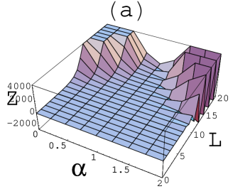
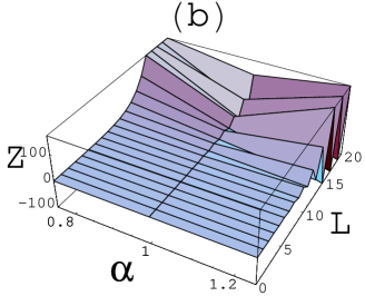
Figure 1: The figure shows a 3D plot of the partition function $Z_{L,\alpha}(N)$ of the linear interacting matrix model of RNA as a function of $\alpha(=0,0.25,0.5,0.75,1)$ and $L$ (upto 20) in (a). The plot in (b) magnifies the $\alpha=0.75,1,1.25$ region. At $\alpha=1$, $Z_{L,\alpha}(N)$ has a finite non-zero value for even lengths whereas it is zero for odd lengths.

The parameter $\alpha$ in Eq. (12) appears only in the exponent. The partition functions for different $L$ and $\alpha$ can be obtained by comparing powers of $t$ on both the sides of Eq. (12) (Table I) and is shown in Fig. 1(a) for $L\leq 20$ and $0\leq\alpha\leq 2$ (raised in intervals of 0.25). For $\alpha=1$, only even $L$ partition functions are non-zero whereas the odd $L$ partition functions vanish (Fig. 1(b)). For completeness we give the explicit dependence of partition function $Z_{L,\alpha}(N)$ on $N$ in terms of the topological parameter, genus $g$, as $Z_{L,\alpha}(N)=\sum_{g=0}^{\infty}a_{L,g,\alpha}\frac{1}{N^{2g}}$ 11 . Here the coefficients $a_{L,g,\alpha}$ give the weighted number of diagrams at a given $L$, genus $g$ and $\alpha$. Also, the total weighted number of diagrams are given by ${\cal N}_{\alpha}=Z_{L,\alpha}(N=1)$, for a particular $L$ and $\alpha$, independent of the genus.

It is found on doing the matrix integrals, that the partition function and weight of any configuration (Feynman diagram) are both positive for the interaction parameter $\alpha$ when $0\leq\alpha\leq 1$, listed in Table I. But when $\alpha>1$, the partition function and weights of Feynman diagrams become negative for odd lengths of the chain, however they still remain positive for the even lengths. Since each Feynman diagram represents a conformation of RNA which must have a non-negative weight, Feynman diagrams of the matrix model with linear external interaction correspond to RNA structures for $0\leq\alpha\leq 1$ for odd $L$ and for all values of $\alpha$ for even $L$.

Table 1: The Table lists partition functions $Z_{L,\alpha}(N)$ for different lengths $L$ at any $\alpha$ for the linear interacting matrix model of RNA.

$L$	$Z_{L,\alpha}(N)$
1	$(1-\alpha$)
2	$(1-\alpha)^{2}+v$
3	$(1-\alpha)^{3}+3v(1-\alpha)$
4	$(1-\alpha)^{4}+6v(1-\alpha)^{2}+2v^{2}+v^{2}/N^{2}$
5	$(1-\alpha)^{5}+10v(1-\alpha)^{3}+10v^{2}(1-\alpha)+5v^{2}(1-\alpha)/N^{2}$
6	$(1-\alpha)^{6}+15v(1-\alpha)^{4}+30v^{2}(1-\alpha)^{2}+15v^{2}(1-\alpha)^{2}/N^{2}+5v^{3}+10v^{3}/N^{2}$
7	$(1-\alpha)^{7}+21v(1-\alpha)^{5}+70v^{2}(1-\alpha)^{3}+35v^{2}(1-\alpha)^{3}/N^{2}+35v^{3}(1-\alpha)$
	$+70v^{3}(1-\alpha)/N^{2}$

II.1 General form of $Z_{L,\alpha}(N)$

The general form of the partition function for the matrix model with linear external interaction can be obtained from Eq. (2) by writing the partition function in terms of the variable $\Phi$ (introduced in section 2) as

$$Z_{L,\alpha}(N)=\frac{1}{\tilde{A}_{L,\alpha}(N)}\int\prod_{i=1}^{L}d\Phi_{i}e^{-\frac{N}{2}Tr[\Phi_{i}(V^{-1})_{ij}\Phi_{j}]}\frac{1}{N}Tr\prod_{i=1}^{L}(1+\Phi_{i}-\alpha),$$ (13)

where $\tilde{A}_{L,\alpha}(N)=\int\prod_{i=1}^{L}d\Phi_{i}exp^{-\frac{N}{2}Tr[\Phi_{i}(V^{-1})_{ij}\Phi_{j}]}$. The general form of $Z_{L,\alpha}(N)$ for the matrix model with linear interaction from Eq. (12) using Wick theorem is

$$Z_{L,\alpha}(N) = (1-\alpha)^{L}+(1-\alpha)^{(L-2)}\sum_{i<j}V_{ij}+(1-\alpha)^{(L-4)}\sum_{i<j<k<l}V_{ij}V_{kl}$$ (14)

$$+(1-\alpha)^{(L-4)}\sum_{i<j<k<l}V_{il}V_{jk}+(\frac{1}{N})^{2}(1-\alpha)^{(L-4)}\sum_{i<j<k<l}V_{ik}V_{jl}$$

$$+....$$

Figure 2: The figure shows all possible diagrams for an RNA chain with length $L=4$ in the linear interacting matrix model of RNA. The paired vertices are connected by dotted arcs and each unpaired vertex is associated with a factor $(1-\alpha)$.

The partition functions for different $\alpha$ at a particular $L$ can be obtained from Eq. (14). This relation has been checked explicitly for $L$ upto 7 from Eq. (2). Each term in the general partition function Eq. (14) is accompanied by powers of $(1-\alpha)$. The partition function corresponding to $L=4$ (Table I) is given by $Z_{L=4,\alpha}(N)=(1-\alpha)^{4}+6v(1-\alpha)^{2}+2v^{2}+v^{2}/N^{2}$. In the Feynman diagram representation 11 , this partition function represents a total of 10 diagrams (Fig. 2) where power of $v$ gives the number of arcs, the coefficients of $v$ give the number of diagrams with those many arcs and power of $(1-\alpha)$ gives the number of unpaired vertices in the diagram. Such terms correspond to planar diagrams. The terms with powers of $1/N^{2}$ represent non-planar diagrams (with crossing arcs) which have non-zero genus. The first term in $Z_{L=4,\alpha}(N)$ is a planar term with no arcs ($v^{0}$) and each unpaired vertex (4 in number) associated with a factor $(1-\alpha)$, the second term represents 6 diagrams with one arc each ($v^{1}$) and each unpaired vertex (2 in number) accompanied by $(1-\alpha)$, the third term corresponds to two diagrams with two arcs each ($v^{2}$) and no unpaired vertex at all and the last term represents one diagram with two crossing arcs ($v^{2}$ and $1/N^{2}$) i.e., a tertiary term with genus one and no unpaired vertices. For $\alpha=1$, the partition function for $L=4$ is given by $Z_{L=4,\alpha=1}(N)=2v^{2}+v^{2}/N^{2}$ (Table I) i.e., a total of 3 Feynman diagrams (in Fig. 2, the diagrams corresponding to $v^{2}$ for $g=0$ and $g=1$). For this $\alpha$ value, only those diagrams with completely paired vertices remain. Thus the structures in the model can be separated in two regimes as (i). $0\leq\alpha<1$ which comprises of Feynman diagrams with both paired and unpaired vertices and (ii). $\alpha=1$ with only completely paired vertices. In (i). different genus structures with different weights (powers of ($1-\alpha$)) associated with each unpaired vertex (($1-\alpha$)) for different $\alpha$’s are included. The completely paired structures in (ii). consist of only those structures which have no unpaired vertices at all.

If now $N=1$ is considered, the general partition function Eq. (14) becomes $Z_{L,\alpha}(N)=(1-\alpha)^{L}+(1-\alpha)^{L-2}\sum_{i<j}V_{ij}+(1-\alpha)^{L-4}\sum_{i<j<k<l}V_{ij}V_{kl}+(1-\alpha)^{L-4}\sum_{i<j<k<l}V_{ik}V_{jl}+....$ For an RNA chain in three dimensions, the partition function can be written as ${\cal Z}=\int\prod_{k=1}^{L}d^{3}r_{k}f(\{r\})Z_{L}(\{r\})$ where $r_{k}$ gives the position of the $k$-th nucleotide in the chain, $f(\{r\})$ is a model dependent function of geometry of the molecule and accounts for steric constraints of the chain, $Z_{L}(\{r\})$ is the partial partition function where pairing between nucleotides comes with a factor $V_{ij}(r_{ij})$ and the coupling constant of each unpaired and paired nucleotide is 1 6 ; 11 . If all steric constraints [$f(\{r\})$] and spatial degrees of freedom ($r_{ij}$) are neglected and the chain is assumed to be infinitely flexible, the partition function becomes ${\cal Z}=Z_{L}=1+\sum_{i<j}V_{ij}+\sum_{i<j<k<l}V_{ij}V_{kl}+\sum_{i<j<k<l}V_{ik}V_{jl}+....$ where $V_{ij}=\rm e^{-\beta\epsilon_{ij}}$. The equation differs from the matrix model partition function Eq. (6) in 6 or Eq. (14) in the powers of $1/N^{2}$ which classify terms with different topological character. Now, if it is assumed that each unpaired nucleotide in $Z_{L}$ is associated with a weight $y$, then ${\cal Z}=Z_{L}=Z_{L,y}=y^{L}+y^{(L-2)}\sum_{i<j}V_{ij}+y^{(L-4)}\sum_{i<j<k<l}V_{ij}V_{kl}+y^{(L-4)}\sum_{i<j<k<l}V_{ik}V_{jl}+....$. The external linear interaction is found to produce this weight on all unpaired bases in partition function of the chain, Eq. (14). Therefore, one can relate the partition function of the linear interacting random matrix model to that of an RNA with $L$ nucleotides in three dimensions where each unpaired base comes with a weight $y=(1-\alpha)$.

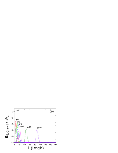
Figure 3: The figure plots genus distribution functions when $\alpha=1$ for the weighted normalized diagrams $a_{L,g,\alpha}/{\cal N}_{\alpha}$ with (a). length $L$ keeping genus $g$ fixed ($g=0,1,2,3,4,10,20$), and (b) genus $g$ with $L$ fixed ($L=40,80,120,160$).

II.2 Genus distribution functions

The genus distribution functions are studied to observe the effect of external linear interaction on the distribution of pseudoknots among the structures of RNA. Figure 3 shows the genus distributions for $\alpha=1$ where Fig. 3(a) plots the weighted normalized diagrams $a_{L,g,\alpha=1}/{\cal N}_{\alpha}$ verses $L$ at fixed genus and Fig. 3(b) shows the weighted normalized diagrams $a_{L,g,\alpha=1}/{\cal N}_{\alpha}$ verses $g$ at a particular $L$. In Fig. 4 the genus distributions are plotted for $\alpha=0,0.75,1$ for: (i). a pair of successive even and odd length $L=(10,11)$ by varying $g$ [Fig. 4(a) and Fig. 4(b)] and (ii). different $L$ at a fixed $g=(0,3)$ [Fig. 4(c) and Fig. 4(d)]. For a chosen $L$, plots for $\alpha=0,0.75,1$ are compared in Fig. 4(a) and Fig. 4(b). In the odd $L=11$ plot, the $\alpha=1$ curve is absent (due to the absence of partition function for odd $L$’s at $\alpha=1$, Table I). It is observed that the curve corresponding to $\alpha=0.75$ in the $L=11$ plot comprises of points which are an average of points in the $\alpha=0.75$ and $\alpha=1$ curves when $L=10$ (same genus points for the two $L$ are considered). For example in Fig. 4(a), the points corresponding to $g=2$ for $\alpha=0.75$ and $\alpha=1$ curves are averaged and the $a_{L,g,\alpha}/{\cal N}_{\alpha}$ value obtained is similar to the $a_{L,g,\alpha}/{\cal N}_{\alpha}$ value for $g=2$ in the $\alpha=0.75$ curve in Fig. 4(b). The same is observed for other such even and odd length comparisons and also when $a_{L,g,\alpha}/{\cal N}_{\alpha}$ is plotted with $L$ for fixed genus, $g=(0,3)$ (Fig. 4(c) and Fig. 4(d)). Notice that for $\alpha=0.75$ in the fixed $g$ plots, the points for each successive even and odd $L$ lie close together separated by large distances from the nearest neighboring even and odd $L$ pair. The values of the weighted normalized distribution can be found from these figures, for example, in Fig. 4(c) for $a_{L=4,g=0,\alpha=0}=9$ and ${\cal N}_{\alpha=0}=10$, $a_{L=4,g=0,\alpha=0}/{\cal N}_{\alpha=0}=0.9$ and for $a_{L=4,g=0,\alpha=1}=2$ and ${\cal N}_{\alpha=1}=3$, $a_{L=4,g=0,\alpha=1}/{\cal N}_{\alpha=1}=0.66$. It is also found numerically that the maximum value of genus $g$ for the matrix model with linear external interaction is $g\leq L/4$ for even $L$ and all $\alpha$ and for odd $L$ and $0\leq\alpha<1$, while for $\alpha=1$ there are no structures.

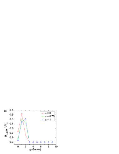
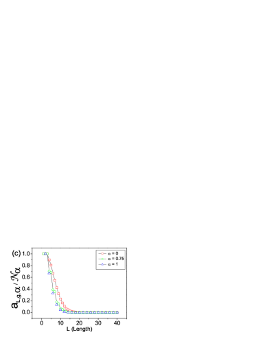
Figure 4: Genus distributions for the weighted normalized diagrams $a_{L,g,\alpha}/{\cal N}_{\alpha}$ are plotted for $\alpha=0,0.75,1$ when (a). $L=10$ and (b). $L=11$ at a fixed genus and (c). $g=0$ and (d). $g=3$ at a fixed length. For odd $L$ ($L=11$) the $\alpha=1$ distribution is absent.

A small length even and odd behavior of the partition function starts emerging as $\alpha$ is increased from 0 towards 1 and becomes very distinct at $\alpha=0.75$. This behavior is more and more prominent for $\alpha$’s greater than 0.75 and in the close vicinity of $\alpha=1$. The random matrix model with a linear external interaction therefore shows small differences in the even and odd $L$ partition function at small $L$. The length scale in the linear interacting matrix model of RNA, below which the even and odd length partition functions are distinguishable, depends upon the interaction parameter $\alpha$ and is found to be $L_{\alpha}\sim 1/(1-\alpha)^{2}$.

III Some interesting results in the random matrix models of RNA

III.1 Scaling relation between the linear interacting and re-scaled random matrix models of RNA

Starting with the generalized partition function $Z_{L,\alpha}(N)$ equation (14) and factoring out $(1-\alpha)^{L}$ from each term results in

$$Z_{L}(v,\alpha,N) = (1-\alpha)^{L}[1+(1-\alpha)^{-2}\sum_{i<j}V_{i,j}+(1-\alpha)^{-4}\sum_{i<j<k<l}V_{ij}V_{kl}$$ (15)

$$+(1-\alpha)^{-4}\sum_{i<j<k<l}V_{il}V_{jk}+(\frac{1}{N})^{2}(1-\alpha)^{-4}\sum_{i<j<k<l}V_{ik}V_{jl}$$

$$+....].$$

The partition function is written with $v$ and $\alpha$ in the argument as its dependence on these parameters will be discussed here. The bracketed quantity on the right hand side of Eq. (15) is the generalized partition function of the random matrix model of RNA ($\alpha=0$) where base pairing interaction strength $v$ has been re-scaled by $(1-\alpha)^{-2}$. The general partition function of the matrix model of RNA with a linear external interaction can thus be written as

$$Z_{L}(v,\alpha,N)=(1-\alpha)^{L}Z_{L}[\frac{v}{(1-\alpha)^{2}},0,N].$$ (16)

This is the scaling theory for the partition function of the random matrix model of RNA with linear external interaction with scale factor $(1-\alpha)^{L}$ having a scaling exponent L and a crossover exponent 2. Such scaling relations have been found in other systems like the anisotropic magnetic systems 21 ; 22 ; 23 ; 24 (section 4 of the first reference in 22 , equations (6-10) of the second reference in 22 and equation (5.4) in 23 ) but in the context of random matrix models such a scaling form has not been observed before in the literature (to the best of our knowledge). For the $\alpha=0$ partition function, which corresponds to the $\alpha=0$ line in Fig. 1(a), re-scaling $v$ by $(1-\alpha)^{-2}$ and multiplying by $(1-\alpha)^{L}$ will give the other $\alpha\neq 0$ lines in Fig. 1(a) as well as the $\alpha=1$ line where $Z_{L,\alpha}(N)=0$ for odd lengths. The distribution functions (Fig. 3 and Fig. 4) can be equivalently studied from the re-scaled random matrix model of RNA for different $\alpha$ values. The matrix model of RNA with linear external interaction can thus be viewed in two equivalent ways, (i). the linear interacting matrix model of RNA where addition of a linear external interaction in the action of the partition function 11 results in each free base of the chain getting weighed by $(1-\alpha)$ and (ii). the random matrix model of RNA where the base pairing strength $v$ is re-scaled by a factor $(1-\alpha)^{-2}$ with an overall scale factor $(1-\alpha)^{L}$. In the present work, the first view point is followed as it incorporates the study of many more general interactions and their effects using the formalism presented here. The addition of more complicated interactions in the matrix model action in general, will not produce such a scaling relationship.

III.2 Thermodynamics

Thermodynamic properties such as the free energy and specific heat for the linear interacting matrix model or equivalently the re-scaled random matrix model of RNA are calculated as functions of length of the chain $L$ (which may be useful in stretching experiments), $\alpha$ and temperature $T$ from Eq. (12). The partition function $Z_{L,\alpha}(N)$ depends upon temperature $T$ through $v$ which is given by $v=e^{-\beta\epsilon}$. The Boltzmann constant, $k_{B}$, and $\epsilon$ are set equal to unity. The calculations are performed with $T=2$ (except for where the $T$ dependence is studied) and $N=100$ and it is expected that the analysis will go through for very large $N$. In the re-scaled random matrix model of RNA, the $\alpha=1$ line corresponds to the limit $v^{\prime}\rightarrow\infty$ as $v^{\prime}$ is given by $v^{\prime}=v/(1-\alpha)^{2}$. Thermodynamic properties (free energy, chemical potential and specific heat) of the model in 11 have been calculated and discussed in 10 as a function of temperature $T$.

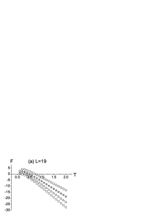
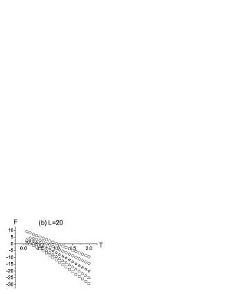
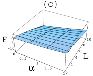
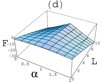
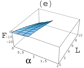
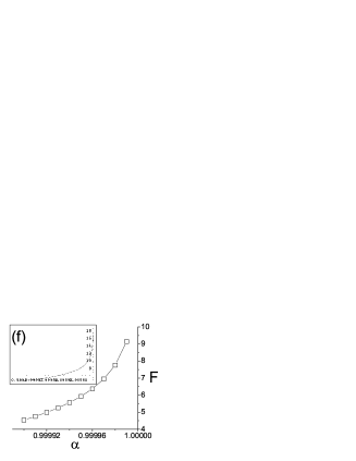
Figure 5: The figure plots free energy as a function of temperature $T$ for (a). $L=19$ and (b). $L=20$ (the $\alpha=1$ curve is absent in (a) as $F$ is imaginary). Plots in (c,e) show $F$ with $L$ and $\alpha$ in a 3D plot. Plot (c) shows all lengths (both even and odd) where the small $L$ even and odd behavior is seen, plot (d) shows only the even lengths and plot (e) shows $F$ for odd lengths only. The $F$ verses $\alpha$ plot in (f) for $L=19$ shows a cusp (inset) as $\alpha\rightarrow 1^{-}$. The symbols in plots (a) and (b) correspond to the following $\alpha$ values: Box $\rightarrow\alpha=0$, Triangle $\rightarrow\alpha=0.25$, Star $\rightarrow\alpha=0.5$, Diamond $\rightarrow\alpha=0.75$ and Pentagon $\rightarrow\alpha=1$.

III.2.1 Free energy and phase transition

The free energy $F$ is found numerically from the partition function $Z_{L,\alpha}(N)$ Eq. (12) using the relation $F_{L,\alpha}(T,N)=-\frac{1}{\beta}ln[Z_{L,\alpha}(T,N)]$. As a function of $T$, the free energy is shown in Fig. 5 for $L=19$ and $L=20$. The curves for different $\alpha$, for both even and odd lengths, lie above the preceding smaller $\alpha$ as $\alpha\rightarrow 1$. The free energy curve for $\alpha=0$ starts from zero at low temperatures and remains negative as $T$ is increased. For $0<\alpha<1$, $F$ at small $T$ rises from zero to a peak $+F$ value and falls down before crossing over to the $-F$ region. The $\alpha=1$ curve (in the $L=20$ plot) starts from a non-zero $+F$ value and drops gradually to the $-F$ side. The $\alpha=1$ curve is absent in the $L=19$ plot as $F$ becomes imaginary. The positive to negative crossover of $F$ for different $\alpha$ is at different $T$ given by $T_{\alpha}\sim\alpha$. This identifies a low and high temperature behavior of $F$ with $T$ for different $\alpha$’s. Three dimensional plots of $F$ with length of the chain $L$ and $\alpha$ are shown in Fig. 5(c)-Fig. 5(e). The small $L$ even and odd behavior of the partition function (discussed in Section 2.2) is visible in Fig. 5(c). Figure 5(d) shows $F$ plotted with only the even lengths and $\alpha$. At small lengths for $\alpha=1$, the plot is flatter compared to relatively large lengths where it is sharply peaked. The peak value however becomes more negative with increasing $L$. It is expected that as length is increased further, the peak will become more and more sharp near $\alpha=1$. This gives signature of a phase transition, at very large $L$, at the $\alpha=1$ line for the even lengths. The free energy for odd lengths and different $\alpha$ in Fig. 5(e) shows that $F$ becomes imaginary at $\alpha=1$. The peaked behavior is present for all, small and large, $L$ with the peak getting sharper for larger lengths. In Fig. 5(f), the cusp from the $\alpha\rightarrow 1^{-}$ side for $F$ is displayed for a particular $L=19$. Hence, for odd lengths the free energy exhibits a phase transition in the linear matrix model of RNA. In order to understand the transition better, the first derivative of free energy with respect to $\alpha$ as a function of $\alpha$ is shown for different $L$ in Fig. 6 (Fig. 6(a) for $L=9,19$ and Fig. 6(b) for $L=10,20$). For the odd length plot in (a), the $L=9$ and $L=19$ curves rise smoothly as $\alpha$ is increased from $0$ towards $1$. But in the very close vicinity of $\alpha=1$, the curves show a steep rise with the values at $\alpha=1$ being very large (Fig. 6(a)). The curves however are seen to pass through zero very close to $\alpha=1$. In the even length plot (b), the $L=10$ and $L=20$ curves behave similar to plot (a) for $\alpha$ from $0$ to near $1$ but suddenly goes down to approximately zero very close to $\alpha=1$. These plots indicate a different behavior for the odd and even lengths near $\alpha=1$. The scaling found in Eq. (18) and discussed in Fig. 1(a) is also present close to the transition line $\alpha=1$.

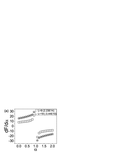
Figure 6: The figure shows first derivative of free energy, $(dF/d\alpha)$, with respect to $\alpha$ for a pair of odd ($L=9,19$) and even lengths ($L=10,20$). The numbers in bracket of the legend of each plot correspond to the numerical $\alpha=1$ values.

III.2.2 Specific heat

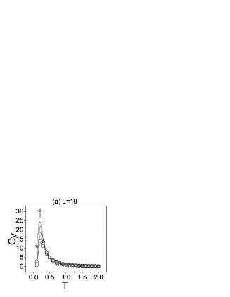
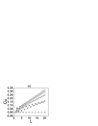
Figure 7: The figure shows specific heat $C_{v}$, for $\alpha=0,0.25,0.5,0.75,1$, plotted as a function of (i). temperature $T$ for (a). $L=19$ and (b). $L=20$ (with $\alpha=1$ plot in the inset) and (ii). length $L$. The different $\alpha$ curves lie one above (below) the other when plotted as a function of $T$ (length) as $\alpha\rightarrow 1$. The symbols in the plots correspond to the following $\alpha$: Box $\rightarrow\alpha=0$, Circle $\rightarrow\alpha=0.25$, Triangle $\rightarrow\alpha=0.5$, Star $\rightarrow\alpha=0.75$ and Pentagon $\rightarrow\alpha=1$.

The specific heat can be found from the free energy as $C_{v}=-T\partial^{2}F/\partial T^{2}$ where constant volume implies constant $L$ here. The $C_{v}$ verses $T$ plots for different $\alpha(=0,0.25,0.5,0.75,1)$ and a pair of odd ($L=19$) and even ($L=20$) lengths is shown in Fig. 7(a) and Fig. 7(b) respectively. The curves for different $\alpha$ lie above the preceding $\alpha$ curve as $\alpha\rightarrow 1$. The maximum $C_{v}$ for different $\alpha$ curves increases as $\alpha$ is increased towards 1. For $L=19$, the $\alpha=1$ curve is absent as free energy is imaginary (as discussed above). The $\alpha=1$ plot for $L=20$, shown as an inset to Fig. 7(b), is indeterminate at $T=0$ and oscillates wildly at low $T$. The scale of the inset ($\alpha=1$) is of the order $10^{-12}$ smaller than the other $\alpha\neq 1$ curves. As a function of $L$, $C_{v}$ is plotted for different $\alpha$ values in Fig. 7(c). At small lengths, the even and odd behavior (as found in the genus distribution functions) can be observed in this plot as $\alpha$ approaches 1. The different $\alpha\neq 0$ curves lie below the preceding $\alpha$ curve. In the $\alpha=1$ curve, $C_{v}$ for odd lengths is indeterminate and is zero for even lengths. To explore the behavior near $\alpha=1$ line, the first derivative of specific heat with respect to $\alpha$, $dC_{v}/d\alpha$, plotted as a function of $\alpha$ is shown in Fig. 8 (Fig. 8(a) for $L=9,19$ and Fig. 8(b) for $L=10,20$). In the odd length plot (a), the $L=9$ curve bells down very near $\alpha=1$ and the $L=19$ curve shows a rising behavior with very large values in the close vicinity of $\alpha=1$. The curves however pass through zero very near $\alpha=1$. The plot (d) shows a smooth rise initially which shoots upward sharply near $\alpha=1$ and drops to approximately zero at $\alpha=1$. This again indicates a different behavior for the odd and even lengths near $\alpha=1$.

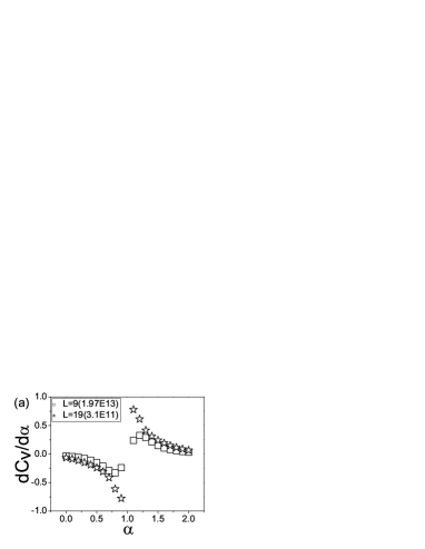
Figure 8: The first derivative of specific heat, $(dC_{v}/d\alpha)$, with respect to $\alpha$ for a pair of odd ($L=9,19$) and even lengths ($L=10,20$) is shown. The numbers in bracket of the legend (in each plot) correspond to the numerical $\alpha=1$ values for the particular length curves.

Therefore, it is observed that as the length is increased, the plots (for both $F$ and $C_{v}$) become more sharply peaked near $\alpha=1$. It is expected that as one goes to very large lengths (of the order of hundreds of bases), the derivatives with respect to $\alpha$ as a function of $\alpha$ will be discontinuous as they approach (i). $+\infty$ and $-\infty$ for $dF/d\alpha$ and (ii). $-\infty$ and $+\infty$ for $dC_{v}/d\alpha$ when $\alpha\rightarrow 1^{-}$ and $1^{+}$ respectively (for the odd lengths see also Fig. 5(f)). The transition for the odd and even lengths seem to be different. In order to completely establish the phase transition in these matrix models of RNA and to make the numerical results presented here more concrete, a detailed analytical study for small $L$ and near $\alpha=1$ is required. Moreover, the appearance of a small $L$ even and odd behavior in the distribution functions, free energy and specific heat needs further understanding since these matrix models are models of RNA and hence this phenomena is a possible prediction for real very small RNAs (very little experimental work has been done in this direction).

IV CONCLUSIONS

An analytic calculation of the partition function after introducing a linear external perturbation in the action of the partition function of the random matrix model of RNA in 11 is given. A perturbation parameter $\alpha$ is found which can be tuned to different values to get two different structural regimes in the model. The presence of different regimes was seen in the study of (secondary structures of the) RNA-like polymer models 25 . In this work, different regimes are found with tertiary structures taken into account in addition to the secondary structures. The structural changes between two regimes with respect to $\alpha$ can be defined as comprising of (i). unpaired and paired base structures, in the regime $0\leq\alpha<1$ and (ii). completely paired base structures when $\alpha=1$. The regime (i) is like the molten phase of the RNA structures shown by many statistical models of RNA (see for example 26 ). The fully paired regime corresponds to a range of structures (similar to the fully paired regime discussed in 25 ). The general form of $Z_{L,\alpha}(N)$ has terms weighted by powers of $(1-\alpha)$. The linear perturbation $W_{i}=w$ introduced in the action of the partition function in Eq. (2) thus alters the contribution of unpaired bases as compared to the paired ones. In the linear interacting model picture, a physical effect which gives rise to $w$ can be the different surroundings of the cell in which the RNA lives such as the presence of ions or molecules 27 ; 28 ; 29 , then $(1-\alpha)$ represents this change. The interaction introduced here may have other concrete realizations, for example in the pulling experiments (5 ; 30 and references therein). The genus distributions at different $L$, $\alpha$ and genus $g$ exhibit small differences for, even and odd, short lengths with these differences disappearing at long lengths in the partition function.

It is observed that the linear interacting matrix model is related via a scaling expression to the random matrix model of RNA where the base pairing interaction strength $v$ has been re-scaled by $(1-\alpha)^{-2}$. The two approaches are equivalent in this sense. The thermodynamic variables (free energy and specific heat) as a function of (i). $L$ show a different even and odd length character present in the model, which may be of interest in the stretching experiments, (ii). $T$ show a different low and high temperature behavior in the free energy. The analysis of the free energy of the interacting matrix model with respect to $\alpha$ shows a phase transition for the odd lengths and a sharp transition is expected for the large even lengths. A detailed analytic study of the phase transition reported here (found numerically) in these matrix models of RNA is for a future work.

The formalism gives a systematic analytical method of studying the effect of external interactions on the number of the planar and non-planar diagrams for a given $L$ and on their thermodynamic properties. These models are matrix models of RNA which enumerate structures of all types that are possible for a given length of the chain. So the characteristics observed in the distribution functions and the thermodynamics, like the small $L$ even and odd behavior, should be found in some real RNA’s such as the micro-RNA which are small with only 21-23 nucleotides. The results found here are also interesting in their own right purely from the point of view of random matrix theory.

References

- (1) E. Westhof, P. Auffinger, Encyclopedia of Analytical Chemistry (Ed., R. A. Meyers) (John Wiley & Sons Ltd, Chichester, 2000) pp. 5222.
- (2) M. Pillsbury, H. Orland, A. Zee, Phys. Rev. E 72, 011911 (2005); M. Pillsbury, J. A. Taylor, H. Orland, A. Zee, cond-mat/0310505.
- (3) J. P. Abrahams, M. van den Berg, E. van Batenburg, C. W. A. Pleij, Nucleic Acids Res. 18, 3035 (1990); A. P. Gultyaev, Nucleic Acids Res. 19, 2489-2494 (1991).
- (4) A. C. Forster, S. Altman, Cell 62, 407-408 (1990); I. Brierley, N. J. Rolley, A. J. Jenner, S. C. Inglis, J. Mol. Biol 220, 889-902 (1991); J. W. Brown, Biochemie 73, 689 (1991); J. D. Dinman, T. Icho, R. B.Wickner, Proc. Natl. Acad. Sci. USA 88, 174-178 (1991); E. S. Haas, D. P. Morse, J. W. Brown, J. F. Schmidt, N. R. Pace, Science 254, 853-856 (1991); N. Wills, R. F. Gesteland, J. F. Atkins, Proc. Natl. Acad. Sci. USA 88, 6991-6995 (1991); M. Chamorro, N. Parkin, H. E. Varmus, Proc. Natl. Acad. Sci. USA 89, 713-717 (1992); E. Westhof, L. Jaeger, Current Opinion Struct. Biol. 2, 327-333 (1992); A. Loria, T. Pan, RNA 2, 551-563 (1996).
- (5) J. F. Marko, E. D. Siggia, Macromolecules 28, 8759-8770 (1995); D. Thirumalai, S. A. Woodson, Acc. Chem. Res. 29, 433 (1996); U. Bockelmann, B. Essevaz-Roulet, F. Heslot, Phys. Rev. Lett. 79, 4489-4492 (1997); U. Bockelmann, B. Essevaz-Roulet, F. Heslot, Phys. Rev. E 58, 2386-2394 (1998); J. Liphardt, B. Onoa, S. B. Smith, I. Tinoco, C. Bustamante, Science 292, 733-737 (2001); M. Muller, F. Krzakala, M. Mezard, Euro. Phys. J. E 9, 67-78 (2002); P. Leoni, C. Vanderzande, Phys. Rev. E 68, 051904 (2003); C. Hyeon, D. Thirumalai, Proc. Natl. Acad. Sci. USA 102, 6789-6794 (2005); F. David, C. Hagendorf, K. -J. Wiese, Eur. Phys. Lett. 78, 68003 (2007).
- (6) Henri Orland, A. Zee, Nucl. Phys. B620[FS], 456-476 (2002).
- (7) C. W. Pleij, K. Rietveld, L. Bosch, Nucleic Acids Res. 13, 1717-1731 (1985); L. X. Shen, I. Tinoco Jr., J. Mol. Biol. 247, 963-978 (1995); P. L. Adams, M. R. Stahley, A. B. Kosek, J. Wang, S. A. Strobel, Nature 430, 45-50 (2004).
- (8) G. ’t Hooft, Nucl. Phys. B72, 461-473 (1974); Nucl. Phys. B75, 461 (1974).
- (9) A. Zee, Acta Physica Polonica B 36, 2829-2836 (2005); G. Vernizzi, H. Orland, Acta Physica Polonica B 36, 2821-2827 (2005).
- (10) M. G. dell’Erba, G. R. Zemba, Phys. Rev. E 79, 011913 (2009).
- (11) G. Vernizzi, H. Orland, A. Zee, Phys. Rev. Lett. 94, 168103 (2005).
- (12) P. -G. de Gennes, Biopolymers 6, 715-729 (1968).
- (13) M. Muller, Phys. Rev. E 67, 021914 (2003).
- (14) T. R. Einert, P. Nager, H. Orland, R. R. Netz, Phys. Rev. Lett. 101, 048103 (2008).
- (15) P. G. Higgs, Association of Asia Pacific Physics Societies (AAPPS) Bulletin 13 (2), 2003; R. Blossey, Computational Biology: A Statistical Mechanics Perspective (Chapman & Hall/CRC, London, 2006), Chapter 3; R. Bundschuh, U. Gerland, Eur. Phys. J. E. 19, 319-330 (2006).
- (16) M. Bon, G. Vernizzi, H. Orland, A. Zee, J. Mol. Biol. 379, 900-911 (2008).
- (17) C. Nappi, Mod. Phys. Lett. A5, 2773-2776 (1990).
- (18) M. L. Mehta, Random Matrices and the Statistical Theory of Energy Levels, second ed., Academic, New York, 1991.
- (19) G. Akemann, G. M. Cicuta, L. Molinari, G. Vernizzi, Phys. Rev. E 59, 1489-1497 (1999).
- (20) I. S. Gradshteyn, I. M. Ryzhik, Table of Integrals, Series and Products, seventh ed., Academic, New York, 1965, pp. 837.
- (21) P. G. de Gennes, Scaling Concepts in Polymer Physics, Cornell University Press, Ithaca and London, 1979, Part C, Chapters X and XI.
- (22) E. Riedel, F. Wegner, Z. Physik 225, 195-215 (1969); Phys. Rev. Lett. 24, 730-733 (1970).
- (23) D. J. Amit, Field Theory, the Renormalization Group, and Critical Phenomenon, second ed., World Scientific, Singapore, 1984, Part II, Chapter 5.
- (24) K. Huang, Statistical Mechanics, second ed., John Wiley & Sons, Singapore, 2000, Chapter 16.
- (25) M. Pretti, Phys. Rev. E 74, 051803 (2006).
- (26) R. Bundschuh, T. Hwa, Europhys. Lett. 59 903-909 (2002).
- (27) D. E. Draper, D. Grilley, A. M. Soto, Annu. Rev. Biophys. Biomol. Struct. 34, 221 (2005).
- (28) I. Tinoco Jr., C. Bustamante, J. Mol. Biol. 293, 271-281 (2003).
- (29) V. K. Misra, D. E. Draper, Biopolymers (Nucl. Acids Sci.) 48, 113-135 (2003).
- (30) I. Garg, N. Deo, Phys. Rev. E 79, 061903 (2009).