Manipulability of Single Transferable Vote
Abstract
For many voting rules, it is NP-hard to compute a successful manipulation. However, NP-hardness only bounds the worst-case complexity. Recent theoretical results suggest that manipulation may often be easy in practice. We study empirically the cost of manipulating the single transferable vote (STV) rule. This was one of the first rules shown to be NP-hard to manipulate. It also appears to be one of the harder rules to manipulate since it involves multiple rounds and since, unlike many other rules, it is NP-hard for a single agent to manipulate without weights on the votes or uncertainty about how the other agents have voted. In almost every election in our experiments, it was easy to compute how a single agent could manipulate the election or to prove that manipulation by a single agent was impossible. It remains an interesting open question if manipulation by a coalition of agents is hard to compute in practice.
1 Introduction
A simple mechanism for collaborating agents to reach consensus on a plan of action is to vote. One issue is the possibility of agents trying to manipulate such an election by mis-reporting their preferences in order to get a better result. Fortunately, it is often computationally difficult to find a successful manipulation [1]. For example, Bartholdi and Orlin proved that the Single Transferable Vote (STV) rule is NP-hard to manipulate [2]. This remains one of the few commonly used voting rules which is NP-hard to manipulate without weights on the votes, or uncertainty in how the other agents have voted. NP-hardness is only a worst-case result and may not reflect the difficulty of manipulation in practice. Indeed, a number of recent theoretical results suggest that manipulation can often be computationally easy [3, 4, 5, 6, 7]. Most recently, Walsh has suggested that empirical studies might provide insights into the computational complexity of manipulation that can complement such theoretical results [8]. For example, when theoretical analysis is asymptotic, empirical studies can reveal if hidden constants and the finite size of elections met in practice are significant. As a second example, theoretical analysis is often restricted to simple distributions. Manipulation may be very different in practice due to correlations between votes. Walsh’s empirical study was limited to the simple veto rule, weighted votes and elections with only three candidates. In this paper, we relax these assumptions and consider the more complex multi-round STV rule, unweighted votes, and large numbers of candidates.
Our experiments suggest that we should treat worst-case results about the complexity of manipulating voting rules like STV with some care. It was easy for a single agent to manipulate almost every election in our experiments or to prove that manipulation by a single agent was impossible. In the millions of elections studied, we computed a manipulation or proved none exists in a few minutes in each case. Indeed, in most cases, we took just a few seconds. As a result, we conjecture that it may be easy for a single agent to compute a manipulation or prove none exists for any STV election involving a hundred or fewer agents and candidates. Since it may be unreasonable or infeasible for an agent to order totally more candidates, and since elections with more agents are usually not manipulable by a single agent, this suggests that manipulation of the STV rule by a single agent is unlikely to be computationally hard in practice.
2 Manipulating STV
Single Transferable Vote (STV) proceeds in a number of rounds. We consider the case of electing a single winner. Each agent totally ranks the candidates. Unless one candidate has a majority of first place votes, we eliminate the candidate with the least number of first place votes. Any ballots placing the eliminated candidate in first place are re-assigned to the second place candidate. We then repeat until one candidate has a majority. STV is used in a wide variety of elections including for the Irish presidency, the Australian House of Representatives, the Academy awards, and many societies and organizations including the American Political Science Association, the International Olympic Committee, and the British Labour Party.
As in previous studies, we assume that the agents manipulating the election know all the other votes. The manipulation problem is to decide how the manipulators should vote, perhaps differently to their true preferences, in order for a chosen candidate to win. Amongst voting rules where the winner is polynomial to compute, STV appears to be one of the harder rules to compute how to manipulate. For example, it is NP-hard to manipulate by a single voter if the number of candidates is unbounded and votes are unweighted [2], or by a coalition of voters if there are 3 or more candidates and votes are weighted (or votes are unweighted but there is uncertainty about the votes) [9]. Coleman and Teague give an enumerative method for a coalition of unweighted voters to compute a manipulation of the STV rule which runs in time where is the number of voters and is the number of candidates [10]. For a single manipulator, Conitzer gave a method to compute the set of candidates that a single agent can make win a STV election which takes time [11]. We improve upon Conitzer’s procedure to compute if a single agent can manipulate a (possibly weighted) STV election to make a desired candidate win. Unlike Conitzer’s procedure, we ignore any election in which the chosen candidate is eliminated, and terminate search as soon as we find any manipulation in which the chosen candidate wins.
3 Uniform votes
We start with one of the simplest possible scenarios: elections in which each vote is equally likely. We have one agent trying to manipulate an election of candidates where other agents vote. Votes are drawn uniformly at random from all possible votes. This is the Impartial Culture (IC) model.
3.1 Varying number of candidates
In Figures 1 and 2, we plot the probability that a manipulator can make a random agent win, and the search to compute if this is possible when we fix the number of agents but vary the number of candidates. In this and subsequent experiments, we tested 1000 problems at each point. Unless otherwise indicated, the number of candidates and the number of agents are varied in powers of 2 from 1 to 128.
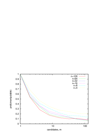
The number of agents voting is fixed and we vary the number of candidates. The fixed votes are uniformly drawn at random from the possible votes. The y-axis measures the probability that the manipulator can make a random candidate win.
As the number of candidates increases, the ability of an agent to manipulate the election decreases. Unlike phase transition behaviour [12] in domains like satisfiability [13, 14], constraint satisfaction [15, 16], number partitioning [17, 18], graph colouring [19, 20] and the traveling salesperson problem [21], the probability curve does not appear to sharpen to a step function around a fixed point. The probability curve resembles the smooth phase transitions seen in polynomial problems like 2-coloring [22] and 1-in-2 satisfiability [23].
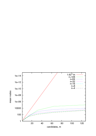
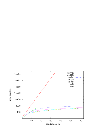
The number of agents voting is fixed and we vary the number of candidates. The y-axis measures the mean number of nodes explored to compute a manipulation or prove that none exists. Median and other percentiles are similar.
Whilst the cost of computing a manipulation increases exponential with the number of candidates , the observed scaling is much better than the . We can easily compute manipulations for up to 128 candidates. There are perhaps few real world elections with more candidates than this. Note that is over for . Thus, we appear to be far from the worst case. We fitted the observed data to the model and found a good fit with and a coefficient of determination, .
3.2 Varying number of agents
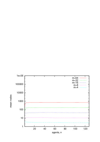
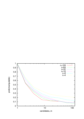
In Figures 3 and 4, we plot the probability that a manipulator can make a random agent win, and the cost to compute if this is possible when we fix the number of candidates but vary the number of agents in the election.
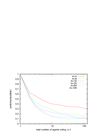
The number of candidates is fixed and we vary the number of agents voting.
The ability of an agent to manipulate the election decreases as the number of agents, increases. Only if there are few votes and few candidates is there a significant chance that the manipulator will be able to change the result. Finding a manipulation or proving none is possible is easy unless we have both a a large number of agents and a large number of candidates. However, in this situation, the chance that the manipulator can change the result is very small.
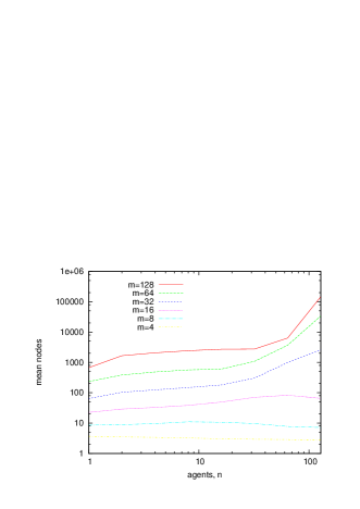
The number of candidates is fixed and we vary the number of agents voting. Median and other percentiles are similar.
4 Urn model
To study the impact of more correlation between votes, we considered random votes drawn from the Polya Eggenberger urn model [24]. In this model, we have an urn containing all possible votes. We draw votes out of the urn at random, and put them back into the urn with additional votes of the same type (where is a parameter). As increases, there is increasing correlation between the votes. This generalizes both the Impartial Culture model () and the Impartial Anonymous Culture () model. To give a parameter independent of problem size, we consider . For instance, with , there is a 50% chance that the second vote is the same as the first.

The number of agents voting is fixed and we vary the number of candidates. The fixed votes are drawn using using the Polya Eggenberger urn model with . The y-axis measures the probability that the manipulator can make a random candidate win.

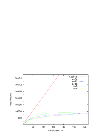
The number of agents voting is fixed and we vary the number of candidates. The fixed votes are drawn using the Polya Eggenberger urn model with . The y-axis measures the mean number of search nodes explored to compute a manipulation or prove that none exists. The curves for different fit closely on top of each other. Median and other percentiles are similar.
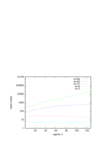
The number of candidates is fixed and we vary the number of agents voting. The fixed votes are drawn using the Polya Eggenberger urn model with . The y-axis measures the mean number of search nodes explored to compute a manipulation or prove that none exists. Median and other percentiles are similar.
In Figures 5 and 6, we plot the probability that a manipulator can make a random agent win, and the cost to compute if this is possible as we vary the number of candidates in an election where votes are drawn from the Polya Eggenberger urn model. The search cost to compute a manipulation increases exponential with the number of candidates . However, we can easily compute manipulations for up to 128 candidates and agents. We fitted the observed data to the model and found a good fit with and a coefficient of determination, .
In Figure 7, we plot the cost to compute a manipulation when we fix the number of candidates but vary the number of agents. As in previous experiments, finding a manipulation or proving none exists is easy even if we have many agents and candidates.
5 Sampling real elections
Elections met in practice may differ from those sampled so far. There might, for instance, be some votes which are never cast. On the other hand, with the models studied so far every possible vote has a non-zero probability of being seen. We therefore sampled some real voting records [25, 26].
The number of agents voting is fixed and we vary the number of candidates. The y-axis measures the probability that the manipulator can make a random candidate win.
The number of agents voting is fixed and we vary the number of candidates. The y-axis measures the mean number of search nodes explored to compute a manipulation or prove that none exists. Median and other percentiles are similar.

The number of candidates is fixed and we vary the number of agents voting. The y-axis measures the mean number of search nodes explored to compute a manipulation or prove that none exists. Median and other percentiles are similar.
Our first experiment uses the votes cast by 10 teams of scientists to select one of 32 different trajectories for NASA’s Mariner spacecraft [27]. Each team ranked the different trajectories based on their scientific value. We sampled these votes. For elections with 10 or fewer agents voting, we simply took a random subset of the 10 votes. For elections with more than 10 agents voting, we simply sampled the 10 votes with uniform frequency. For elections with 32 or fewer candidates, we simply took a random subset of the 32 candidates. Finally for elections with more than 32 candidates, we duplicated each candidate and assigned them the same ranking. Since STV works on total orders, we then forced each agent to break any ties randomly.
In Figures 8 to 10, we plot the probability that a manipulator can make a random agent win, and the cost to compute if this is possible as we vary the number of candidates and agents. Votes are sampled from the NASA experiment as explained earlier. The search needed to compute a manipulation again increases exponential with the number of candidates . However, the observed scaling is much better than . We can easily compute manipulations for up to 128 candidates and agents.
In our second experiment, we used votes from a faculty hiring committee at the University of California at Irvine [28]. This dataset had 10 votes for 3 different candidates. We sampled from this in the same ways as from the NASA dataset. Results are reported in Figures 11 and 12. As in the previous experiments, it was easy to find a manipulation or prove that none exists. The observed scaling was again much better than .
The number of agents voting is fixed and we vary the number of candidates. The y-axis measures the mean number of search nodes explored to compute a manipulation or prove that none exists. Median and other percentiles are similar.
The number of candidates is fixed and we vary the number of agents voting. The y-axis measures the mean number of search nodes explored to compute a manipulation or prove that none exists. Median and other percentiles are similar.
6 Related work
Coleman and Teague proposed algorithms to compute a manipulation for the STV rule [10]. They also conducted an empirical study which demonstrates that only relatively small coalitions are needed to change the elimination order of the STV rule. They observed that most uniform and random elections are not trivially manipulable using a simple greedy heuristic. On the other hand, our results suggest that, for manipulation by a single agent, a limited amount of backtracking is needed to find a manipulation or prove that none exists.
Walsh empirically studied the cost of manipulating the veto rule by a coalition of agents whose votes were weighted [8]. He showed that there was a smooth transition in the probability that a coalition can elect a desired candidate as the size of the manipulating coalition increases. He also showed that it was easy to find manipulations of the veto rule or prove that none exist for many independent and identically distributed votes even when the coalition of manipulators was critical in size. He was able to identify a situation in which manipulation was computationally hard. This is when votes are highly correlated and the election is “hung”. However, even a single uncorrelated voter was enough to make manipulation easy again.
As indicated, there have been several theoretical results recently that suggest elections are easy to manipulate in practice despite NP-hardness results. For instance, Xia and Conitzer have shown that for a large class of voting rules including STV, as the number of agents grows, either the probability that a coalition can manipulate the result is very small (as the coalition is too small), or the probability that they can easily manipulate the result to make any alternative win is very large [5]. They left open only a small interval in the size for the coalition for which the coalition is large enough to be able to manipulate but not obviously large enough to be able to manipulate the result easily.
As a second example, Procaccia and Rosenschein proved that for most scoring rules and a wide variety of distributions over votes, when the size of the coalition is , the probability that they can change the result tends to 0, and when it is , the probability that they can manipulate the result tends to 1 [29]. They also gave a simple greedy procedure that will find a manipulation of a scoring rule in polynomial time with a probability of failure that is an inverse polynomial in [4]. Friedgut, Kalai and Nisan proved that if the voting rule is neutral and far from dictatorial and there are 3 candidates then there exists an agent for whom a random manipulation succeeds with probability [6]. Starting from different assumptions, Xia and Conitzer showed that a random manipulation would succeed with probability for 3 or more candidates for STV, for 4 or more candidates for any scoring rule and for 5 or more candidates for Copeland [7].
7 Conclusions
We have studied empirically whether computational complexity is a barrier to the manipulation for the STV rule. We have looked at a number of different distributions of votes including uniform random votes, correlated votes drawn from an urn model, and votes sampled from some real world elections. We have looked at manipulation by both a single agent, and a coalition of agents who vote in unison. Unlike phase transition behaviour in domains like satisfiability, we did not observe rapid transitions in the manipulability of STV elections that sharpen around a fixed point, but saw instead smooth transitions. We also did not observe hard instances around the transition in manipulability. Indeed, almost every one of the millions of elections in our experiments was easy to manipulate or to prove could not be manipulated. Our results suggest that it may be easy for a single agent to compute a manipulation or prove none is possible for any STV election involving a hundred or fewer of agents and candidates. It would also be interesting to perform a similar empirical study for other voting rules as well as for other types of manipulation and control (e.g. manipulation by a coalition, or control by the addition/deletion of candidates). Two interesting rules to study are maximin and ranked pairs. These two rules have only recently been shown to be NP-hard to manipulate, and are members of the small set of voting rules which are NP-hard to manipulate without weights or uncertainty [30].
References
- [1] Bartholdi, J., Tovey, C., Trick, M.: The computational difficulty of manipulating an election. Social Choice and Welfare 6(3) (1989) 227–241
- [2] Bartholdi, J., Orlin, J.: Single transferable vote resists strategic voting. Social Choice and Welfare 8(4) (1991) 341–354
- [3] Conitzer, V., Sandholm, T.: Nonexistence of voting rules that are usually hard to manipulate. In: Proceedings of the 21st National Conference on AI, Association for Advancement of Artificial Intelligence (2006)
- [4] Procaccia, A.D., Rosenschein, J.S.: Junta distributions and the average-case complexity of manipulating elections. Journal of Artificial Intelligence Research 28 (2007) 157–181
- [5] Xia, L., Conitzer, V.: Generalized scoring rules and the frequency of coalitional manipulability. In: EC ’08: Proceedings of the 9th ACM conference on Electronic commerce, New York, NY, USA, ACM (2008) 109–118
- [6] Friedgut, E., Kalai, G., Nisan, N.: Elections can be manipulated often. In: Proc. 49th FOCS, IEEE Computer Society Press (2008)
- [7] Xia, L., Conitzer, V.: A sufficient condition for voting rules to be frequently manipulable. In: EC ’08: Proceedings of the 9th ACM conference on Electronic commerce, New York, NY, USA, ACM (2008) 99–108
- [8] Walsh, T.: Where are the really hard manipulation problems? The phase transition in manipulating the veto rule. In: Proceedings of 21st IJCAI, International Joint Conference on Artificial Intelligence (2009)
- [9] Conitzer, V., Sandholm, T., Lang, J.: When are elections with few candidates hard to manipulate. Journal of the Association for Computing Machinery 54 (2007)
- [10] Coleman, T., Teague, V.: On the complexity of manipulating elections. In: Proceedings of the 13th The Australasian Theory Symposium (CATS2007). (2007) 25–33
- [11] Conitzer, V.: Computational Aspects of Preference Aggregation. PhD thesis, Computer Science Department, Carnegie Mellon University (2006)
- [12] Cheeseman, P., Kanefsky, B., Taylor, W.: Where the really hard problems are. In: Proceedings of the 12th IJCAI, International Joint Conference on Artificial Intelligence (1991) 331–337
- [13] Mitchell, D., Selman, B., Levesque, H.: Hard and Easy Distributions of SAT Problems. In: Proceedings of the 10th National Conference on AI, Association for Advancement of Artificial Intelligence (1992) 459–465
- [14] Gent, I., Walsh, T.: The SAT phase transition. In Cohn, A.G., ed.: Proceedings of 11th ECAI, John Wiley & Sons (1994) 105–109
- [15] Gent, I., MacIntyre, E., Prosser, P., Walsh, T.: Scaling effects in the CSP phase transition. In: 1st International Conference on Principles and Practices of Constraint Programming (CP-95), Springer-Verlag (1995) 70–87
- [16] Gent, I., MacIntyre, E., Prosser, P., Smith, B., Walsh, T.: Random constraint satisfaction: Flaws and structure. Constraints 6(4) (2001) 345–372
- [17] Gent, I., Walsh, T.: Phase transitions and annealed theories: Number partitioning as a case study. In: Proceedings of 12th ECAI. (1996)
- [18] Gent, I., Walsh, T.: Analysis of heuristics for number partitioning. Computational Intelligence 14(3) (1998) 430–451
- [19] Walsh, T.: Search in a small world. In: Proceedings of 16th IJCAI, International Joint Conference on Artificial Intelligence (1999)
- [20] Walsh, T.: Search on high degree graphs. In: Proceedings of 17th IJCAI, International Joint Conference on Artificial Intelligence (2001)
- [21] Gent, I., Walsh, T.: The TSP phase transition. Artificial Intelligence 88 (1996) 349–358
- [22] Achlioptas, D.: Threshold phenomena in random graph colouring and satisfiability. PhD thesis, Department of Computer Science, University of Toronto (1999)
- [23] Walsh, T.: From P to NP: COL, XOR, NAE, 1-in-k, and Horn SAT. In: Proceedings of the 17th National Conference on AI, Association for Advancement of Artificial Intelligence (2002)
- [24] Berg, S.: Paradox of voting under an urn model: the effect of homogeneity. Public Choice 47 (1985) 377–387
- [25] Gent, I., Walsh, T.: Phase transitions from real computational problems. In: Proceedings of the 8th International Symposium on Artificial Intelligence. (1995) 356–364
- [26] Gent, I., Hoos, H., Prosser, P., Walsh, T.: Morphing: Combining structure and randomness. In: Proceedings of the 16th National Conference on AI, Association for Advancement of Artificial Intelligence (1999)
- [27] Dyer, J., Miles, R.: An actual application of collective choice theory to the selection of trajectories for the mariner jupiter/saturn 1977 project. Operations Research 24(2) (1976) 220–244
- [28] Dobra, J.: An approach to empirical studies of voting paradoxes: An update and extension. Public Choice 41 (1983) 241–250
- [29] Procaccia, A.D., Rosenschein, J.S.: Average-case tractability of manipulation in voting via the fraction of manipulators. In: Proceedings of 6th Intl. Joint Conference on Autonomous Agents and Multiagent Systems (AAMAS-07). (2007) 718–720
- [30] Xia, L., Zuckerman, M., Procaccia, A., Conitzer, V., Rosenschein, J.: Complexity of unweighted coalitional manipulation under some common voting rules. In: Proceedings of 21st IJCAI, International Joint Conference on Artificial Intelligence (2009) 348–353