Thermal effects in the magnetic Casimir-Polder interaction

Abstract

We investigate the magnetic dipole coupling between a metallic surface and an atom in a thermal state, ground state and excited hyperfine state. This interaction results in a repulsive correction and – unlike the electrical dipole contribution – depends sensitively on the Ohmic dissipation in the material.

1 Introduction

Exact knowledge of the Casimir-Polder interaction between an atom and a conducting surface is rapidly becoming important in modern microtrap experiments (atom chips), whose stability is limited by an attractive potential well at sub-micron distances. We investigate here the magnetic dipole contribution to the atom-surface interaction and find it to be repulsive for atoms prepared in certain states. The magnetic Casimir-Polder potential differs greatly from its electrical counterpart, on which previous research has concentrated. Above all, the much smaller transition frequencies lead to a stronger dependence on temperature and the Ohmic dissipation in the material. This results in a strong suppression at distances above the thermal wavelength which is absent in the case of the plasma and, more generally, in superconductors.

The fundamental quantity calculated in this work is the free energy of the magnetic dipole interaction between an atom and a planar surface. For an atom prepared in a state $|a\rangle$ the free energy is given by the expression[1, 2]

$$\mathcal{F}(L,T)=-k_{B}T\sideset{}{{}^{\prime}}{\sum}_{n=0}^{\infty}\beta^{a}_{ij}(\mathrm{i}\xi_{n})\mathcal{H}_{ji}(L,\mathrm{i}\xi_{n})+\sum_{b}n(\omega_{ba})\mu_{i}^{ab}\mu_{j}^{ba}{\rm Re}[\mathcal{H}_{ji}(L,\omega_{ba})]~{},$$ (1)

where $\xi_{n}=2\pi nk_{B}T/\hbar$ are the Matsubara frequencies and the term $n=0$ comes with a weight $\frac{1}{2}$ in the primed sum. The second (resonant) term involves the mean thermal photon number $n(\omega)$ and the magnetic transition dipole matrix $\boldsymbol{\mu}$. The state-specific polarizability is [3, 1]

$$\beta_{ij}^{a}({\omega})=\sum_{b}\frac{\mu_{i}^{ab}\mu_{j}^{ba}}{\hbar}\frac{2\omega_{ba}}{\omega_{ba}^{2}-(\omega+\mathrm{i}0^{+})^{2}}~{},$$ (2)

while $\boldsymbol{\mathcal{H}}$ is the magnetic Green tensor

$$\boldsymbol{\mathcal{H}}(L,\omega)=\frac{\mu_{0}}{8\pi}\int\limits_{0}^{\infty}kdk\,\kappa\left[\left(r_{\rm s}+\frac{\omega^{2}}{c^{2}\kappa^{2}}r_{\rm p}\right)[\boldsymbol{\hat{x}\hat{x}}+\boldsymbol{\hat{y}\hat{y}}]+2\frac{k^{2}}{\kappa^{2}}r_{\rm s}\boldsymbol{\hat{z}\hat{z}}\right]e^{-2\kappa L}~{}.$$ (3)

Here, $\mu_{0}$ is the vacuum permeability, $k$ is the in plane wave vector, $\boldsymbol{\hat{x}\hat{x}}$, $\boldsymbol{\hat{y}\hat{y}}$, $\boldsymbol{\hat{z}\hat{z}}$ are the cartesian dyadic products, and $\kappa=[k^{2}-(\omega+\mathrm{i}0^{+})^{2}/c^{2}]^{1/2}$. The Fresnel reflection amplitudes[4] $r^{\rm s,p}(k,\omega)$ are taken here for a local, isotropic and nonmagnetic ($\mu(\omega)=1$) medium. All information about the optical properties and the Ohmic dissipation in the surface is then encoded in the dielectric function $\varepsilon(\omega)$. We will consider a Drude metal [4] $\varepsilon_{\mathrm{Dr}}(\omega)=1-\omega_{p}^{2}/[\omega(\omega+\mathrm{i}\gamma)]$ with plasma frequency $\omega_{p}$ and dissipation rate $\gamma>0$, independent of temperature. In the dissipationless plasma model, we get $\varepsilon_{\mathrm{pl}}(\omega)$ by setting $\gamma=0$. It can be read as the limiting case of a superconductor[5] well below the transition temperature. For a more thorough discussion of Casimir(-Polder) effects in superconductors, see Refs.Bimonte2009b, Haakh2009b.

2 Casimir-Polder potential in global equilibrium

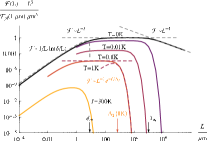
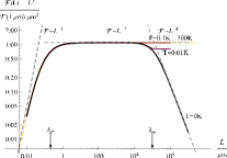
Figure 1: Magnetic Casimir-Polder free energy for a thermalized two-level atom near a Drude metal (left) and a plasma (right). Parameters are $\omega_{p}=8.9\times 10^{15}{\rm s}^{-1},\gamma=0.01\omega_{p},\Omega_{m}=3\times 10^{9}{\rm s}^{-1}\approx 23\,{\rm mK}$. The energy is scaled to $\mathcal{F}_{\rm pl}(1\,\mu{\rm m},0\,{\rm K})=9.79\times 10^{-37}\,\rm J$. Dashed asymptotes: see Ref. Haakh2009b.

For an atom in a thermal state, the polarizability Eq.(2) must be averaged over thermal state occupation numbers. For a two-level system with transition frequency $\Omega_{m}$, this yields

$$\boldsymbol{\beta}^{T}(\omega)=\tanh\left(\frac{\hbar\Omega_{m}}{2k_{B}T}\right)\boldsymbol{\beta}^{g}(\omega)~{},$$ (4)

in terms of the ground state polarizability [Eq. (2) with $a=g$]. In thermal equilibrium, Eq.(1) reduces to

$$\mathcal{F}(L,T)=-k_{B}T\sideset{}{{}^{\prime}}{\sum}_{n=0}^{\infty}\beta^{T}_{ij}(\mathrm{i}\xi_{n})\mathcal{H}_{ji}(L,\mathrm{i}\xi_{n}).$$ (5)

Both $\boldsymbol{\beta}^{T}(\mathrm{i}\xi)$ and $\boldsymbol{\mathcal{H}}(L,\mathrm{i}\xi)$ are real expressions for $\xi>0$. We assume a static magnetic dipole aligned perpendicular to the surface, not unrealistic in magnetic traps, and have $\beta^{T}_{xx}=\beta^{T}_{yy}$ and $\beta^{T}_{zz}=0$.

The free energies for a Drude metal and a plasma are shown in Fig. 1. A striking difference occurs at large distances: the Drude metal is transparent to static magnetic fields [$\boldsymbol{\cal H}(L,0)=0$], and the zeroth term of the Matsubara sum vanishes. The free energy is then dominated by the first term, which decays exponentially for $L>\Lambda_{T}=\hbar c/4\pi k_{B}T$. We call this the thermal decoupling of the magnetic dipole.

A plasma (superconductor) shields static magnetic fields (Meißner-Ochsenfeld effect, $\boldsymbol{\cal H}(L,0)\neq 0$), leading to an enhanced interaction energy at nonzero temperature. The linear dependence on $T$ of the zeroth Matsubara term in Eq. (5) cancels with the thermal polarizability (4) for $\hbar\omega_{ab}\ll k_{B}T$. Only around this (quite low) temperature, there are any thermal effects. [7]. The close coincidence between the thermal and the $T=0$ potentials at small distances can be understood from the low-frequency behaviour of the Green tensor, see Ref. Haakh2009b where also the dashed asymptotes of Fig. 1 are discussed.

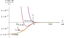
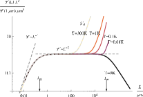
Figure 2: Magnetic Casimir-Polder free energy in the atomic ground state (left: Drude metal, right: plasma). Note the different scaling in the left plot. Parameters as before.

3 Casimir-Polder potential for nonthermal states

Many experimental settings involve atoms prepared in a special state rather than in thermal equilibrium with the environment. We consider a two-level atom prepared in the ground state as an example for an ultracold gas. The assumption $k_{B}T\gg\hbar|\omega_{ba}|$ is quite realistic for most temperatures, and now the resonant part of Eq. (1) contributes, too, and the free energy becomes

$$\mathcal{F}(L,g,T)\approx-2k_{B}T\sum_{n\geq 1}\beta^{g}(\mathrm{i}\xi_{n})\mathcal{H}_{xx}(L,\mathrm{i}\xi_{n})$$ (6)

$${}\qquad+k_{B}T\beta^{g}(0)\left\{{\rm Re}[\mathcal{H}_{xx}(L,\Omega_{m})]-\mathcal{H}_{xx}(L,0)\right\}~{}.$$

At the temperatures considered, the first line (without the $n=0$ term) is nearly identical for the plasma and Drude model. Anyway, the second line is not. In the Drude model $\mathcal{H}(L,0)=0$, but the remaining resonant part is significant in the non-retarded regime. It actually changes the sign of the Casimir-Polder potential already at short distances, as soon as $k_{B}T\gtrsim\hbar\Omega_{m}$, see Fig. 2 (left). This leads to an attractive potential well of approximately $0.02\,\rm{pK}$ [environmental temperature $T=1\,\rm K$] at distances below $1\,\mu\rm m$, possibly accessible to quantum reflection experiments[8]. If we consider an atom prepared in an excited state (e.g. another hyperfine state), the interaction changes sign globally, because of the transition energies $\hbar\omega_{ab}<0$ in the polarizability (2).

In contrast, the magnetic coupling to a plasma is entirely repulsive at small distances (Fig. 2, right). Here, the second line of Eq.(6) nearly vanishes because $\mathcal{H}_{xx}(L,\omega)$ is approximately independent of frequency, at least in the non-retarded regime. Hence, the zeroth Matsubara term is removed from the Casimir-Polder potential and the next order in the expansion of the occupation number $n(\Omega_{m})\approx k_{B}T/\hbar\Omega_{m}-\frac{1}{2}$ gives the leading contribution to the resonant term. In the non-retarded regime this restores the $T=0$ behaviour (cf. right panels of Figs. 1 and 2). At larger distances (retarded regime) the resonant term becomes dominant and oscillates with distance. A scheme to enhance these oscillations for the electric Casimir-Polder interaction has been recently proposed, using rovibrational states of polar molecules[9].

4 Discussion

At experimentally relevant temperatures, the magnetic Casimir-Polder interaction shows much richer effects than its electric counterpart. This is because the electric dipole coupling is dominated by electric fields which in all conductors are screened by surface charges at large scales. This masks any difference between a normal metal and a superconductor (or the plasma model). Differently, the boundary conditions for magnetic fields, relevant for the magnetic dipole, depend on surface currents and hence on Ohmic dissipation. We have seen that including dissipation in the surface response leads to the thermal decoupling of the atom at distances beyond the thermal wavelength. For atoms prepared in a nonthermal state, the balance between repulsive and attractive contributions can produce local extrema, whose sign is controlled by the atomic (hyperfine) state. Experimental tests of the Casimir-Polder interaction may also answer remaining open questions on the temperature dependence of the Casimir interaction, offering the advantage of a well-defined system that can be handled with high precision.

We acknowledge financial support by the European Science Foundation (ESF) within the activity ‘New Trends and Applications of the Casimir Effect’, by the German-Israeli Foundation for Scientific Research and Development (GIF) and by the Alexander von Humboldt foundation.

References

- [1] J. M. Wylie and J. E. Sipe, Phys. Rev. A 32, 2030 (1985).
- [2] M. Gorza and M. Ducloy, Eur. Phys. J. D 40, 343 (2006).
- [3] A. McLachlan, Proc. Roy. Soc. (London) A. 271, 387 (1963).
- [4] J. D. Jackson, Classical electrodynamics (Wiley, New York, 1975).
- [5] J. Schrieffer, Theory of Superconductivity (Perseus Books, 1999).
- [6] G. Bimonte, Phys. Rev. A 78, 062101 (2008).
- [7] H. Haakh, F. Intravaia, C. Henkel, S. Spagnolo, R. Passante, B. Power and F. Sols, submitted to Phys. Rev. A, preprint arXiv:0910.3133 (2009).
- [8] V. Druzhinina and M. DeKieviet, Phys. Rev. Lett. 91, 193202 (2003).
- [9] S. Ellingsen, S. Buhmann and S. Scheel, Phys. Rev. A 80, 22901(2009).