Radiatively Corrected Lepton Energy Distributions in Top Quark Decays $t\to bW^{+}\to b(\ell^{+}\nu_{\ell})$ and $t\to bH^{+}\to b(\tau^{+}\nu_{\tau})$ and single charged prong energy distributions from subsequent $\tau^{+}$ decays

Abstract

We calculate the QED and QCD radiative corrections to the charged lepton energy distributions in the dominant semileptonic decays of the top quark $t\to bW^{+}\to b(\ell^{+}\nu_{\ell})$ $(\ell=e,\mu,\tau)$ in the standard model (SM), and for the decay $t\to bH^{+}\to b(\tau^{+}\nu_{\tau})$ in an extension of the SM having a charged Higgs boson $H^{\pm}$ with $m_{H^{\pm}}<m_{t}-m_{b}$. The QCD corrections are calculated in the leading and next-to-leading logarithmic approximations, but the QED corrections are considered in the leading logarithmic approximation only. These corrections are numerically important for precisely testing the universality of the charged current weak interactions in $t$-quark decays. As the $\tau^{+}$ leptons arising from the decays $W^{+}\to\tau^{+}\nu_{\tau}$ and $H^{+}\to\tau^{+}\nu_{\tau}$ are predominantly left- and right-polarised, respectively, influencing the energy distributions of the decay products in the subsequent decays of the $\tau^{+}$, we work out the effect of the radiative corrections on such distributions in the dominant (one-charged prong) decay channels $\tau^{+}\to\pi^{+}\bar{\nu}_{\tau},\rho^{+}\bar{\nu}_{\tau},a_{1}^{+}\bar{\nu}_{\tau}$ and $\ell^{+}\nu_{\ell}\bar{\nu}_{\tau}$. The inclusive $\pi^{+}$ energy spectra in the decay chains $t\to b(W^{+},H^{+})\to b(\tau^{+}\nu_{\tau})\to b(\pi^{+}\bar{\nu}_{\tau}\nu_{\tau}+X)$ are calculated, which can help in searching for the induced $H^{\pm}$ effects at the Tevatron and the LHC.

I Introduction

Top quark is now firmly established by the experiments CDF and D0 at the $p\bar{p}$ collider Tevatron at Fermilab, with $m_{t}=173.1\pm 1.4$ GeV, decaying dominantly through the mode $t\to bW^{+}\to b(\ell^{+}\nu_{\ell},q\bar{q}^{\prime})$ :2009ec . At the Large Hadron Collider (LHC), expected to be operational shortly, one expects a cross section $\sigma(p\,p\to t\bar{t}X)\simeq 1({\rm nb})$ for the LHC centre of mass energy of 14 TeV Langenfeld:2009tc . With the nominal LHC luminosity of $10^{33}({\rm cm})^{-2}({\rm sec})^{-1}$, one expects a $t\bar{t}$ pair produced per second. The $t\bar{t}$ production cross section for the 10 TeV run of the LHC is estimated as about $0.4$ nb Langenfeld:2009tc , still large enough to undertake dedicated top quark physics. Thus, LHC is potentially a top factory, which will allow to carry out precision tests of the SM and enhance the sensitivity of beyond-the-SM effects in the top quark sector. Anticipating this, a lot of theoretical work has gone into firming up the cross sections for the $t\bar{t}$-pair and the single-top production at the Tevatron and the LHC, undertaken in the form of higher order QCD corrections Moch:2008ai ; Moch:2008qy ; Kidonakis:2008mu ; Cacciari:2008zb . Improved theoretical calculations of the top quark decay width and distributions started a long time ago. The leading order perturbative QCD corrections to the lepton energy spectrum in the decays $t\to bW^{+}\to b(\ell^{+}\nu_{\ell})$ were calculated some thirty years ago Ali:1979is . Subsequent theoretical work leading to analytic derivations implementing the ${\cal O}(\alpha_{s})$ corrections were published in Corbo:1982ah ; Altarelli:1982kh and corrected in Jezabek:1988ja . The order $\alpha_{s}$ contribution to the top quark decay width dominates the radiative corrections (typically -8.5%). The $O(\alpha)$ electroweak corrections contribute typically +1.55%  Denner:1990ns ; Eilam:1991iz , the finite $W$-width effect (-1.56%) almost cancels the electroweak correction Jezabek:1993wk . The next-to-leading order (NLO) QCD corrections in $\alpha_{s}$ (i.e., $\alpha_{s}^{2}$) were computed as an expansion in $(M_{W}/m_{t})^{2}$ in Czarnecki:1998qc ; Chetyrkin:1999ju . These results were confirmed later by an independent analytic calculation in  Blokland:2004ye ; Blokland:2005vq , and contribute about -2.25% to the top quark decay width.

Our main concern in this paper are the lepton energy distributions from the decays $t\to bW^{+}\to b(\ell^{+}\nu_{\ell})$ (for $\ell^{+}=e^{+},\mu^{+},\tau^{+}$), which are modified from their respective Born-level distributions in a way specific for each charged lepton due to the QED corrections. These (QED and QCD) radiative effects have to be taken into account to test the universality of charged current weak interactions in the top quark sector. Another process which breaks the charged lepton universality in the decays $t\to b\ell^{+}\nu_{\ell}$ is induced by charged Higgses $H^{\pm}$ (for $m_{H^{+}}<m_{t}-m_{b}$) in the intermediate state, $t\to bH^{+}\to b(\ell^{+}\nu_{\ell})$, which is expected to influence mainly the final state $b\tau^{+}\nu_{\tau}$ due to the $H^{+}\ell^{+}\nu_{\ell}$ couplings. The leading order in $\alpha_{s}$ corrections to the polarized top quark decay into $H^{+}b$ have been calculated in Korner:2002fx . We study the effects of the radiative corrections on the $\tau^{+}$-energy distribution in the decay $t\to bH^{+}\to b\tau^{+}\nu_{\tau}$.

Radiative (QED and QCD) corrections in the top quark decays, such as $t\to bW^{+}\to b\ell^{+}\nu_{\ell}$, with $\ell^{+}=e^{+},\mu^{+},\tau^{+}$, involve large logarithms due to the large fermion mass ratios. For example, in the leading logarithmic approximation (LLA), one encounters the logarithmic terms

$$L_{e} = \ln\left(\frac{m_{t}^{2}}{m_{e}^{2}}\right)\approx 25.4,\qquad L_{\mu}=\ln\left(\frac{m_{t}^{2}}{m_{\mu}^{2}}\right)\approx 14.8,$$ (1)

$$L_{\tau} = \ln\left(\frac{m_{t}^{2}}{m_{\tau}^{2}}\right)\approx 9.1,\qquad L_{b}=\ln\left(\frac{m_{t}^{2}}{m_{b}^{2}}\right)\approx 7.4,$$

in the partial decay widths. Hence, in the LLA, radiative corrections to the partial widths lead to typically large effects

$$\frac{\alpha}{\pi}L_{e}\approx 6.2~{}\%,\qquad\frac{\alpha}{\pi}L_{\mu}\approx 3.6~{}\%,\qquad\frac{\alpha}{\pi}L_{\tau}\approx 2.1~{}\%,\qquad\frac{\alpha_{s}}{\pi}L_{b}\approx 23~{}\%.$$ (2)

They are included together with the non-logarithmic terms in the estimates undertaken in the fixed order (in $\alpha$ or $\alpha_{s}$) calculations. However, to get perturbatively reliable results, all terms of the type $(\frac{\alpha}{\pi})^{n}\ln\left(\frac{m_{t}^{2}}{m_{e}^{2}}\right)^{n}$ in the decay $t\to be^{+}\nu_{e}$, for example, have to be summed up (the re-summed leading log approximation LLA), as well as $(\frac{\alpha}{\pi})^{n}\ln\left(\frac{m_{t}^{2}}{m_{e}^{2}}\right)^{n-1}$ (the next-to-leading log approximation NLLA). Using the well-studied case of the QED radiative corrections to the purely leptonic decays $\mu^{-}\to\nu_{\mu}e^{-}\bar{\nu}_{e}$, we show that the structure function (SF) approach Lipatov:1974qm ; Altarelli:1977zs (based on the factorisation hypotheses Collins:1984kg ) is the appropriate framework to resum such terms, enabling us to derive the electron energy spectrum with the radiative corrections taken into account to all orders of the large logarithms. As a warm-up exercise, and also to set our notations, we reproduce the well-known results for the QED corrections to the muon decay $\mu^{-}\to e^{-}\bar{\nu}_{e}\nu_{\mu}$ Berman:1958ti ; Kinoshita:1957zz ; Arbuzov:2002pp ; Arbuzov:2002cn and generalise it to all orders of perturbation theory by summing up the leading logs $(\frac{\alpha}{\pi}\ln(m_{\mu}^{2}/m_{e}^{2}))^{n}$ (see Section II). In this context, we also discuss the polarised muon decay case. The SF approach is applied next to the semileptonic decays of the top quark $t\to bW^{+}\to b(\ell^{+}\nu_{\ell})$, where the QCD and QED radiative corrections to the Dalitz (double differential) and inclusive lepton energy distributions are worked out. In this, the QCD-corrected energy distributions are derived in the re-summed leading logarithmic and next-to-leading logarithmic approximations, but the QED corrections to these distributions are calculated in the leading logarithmic approximation only. This is discussed in detail in Section IV.

In many extension of the SM, the Higgs sector of the SM is enlarged, typically by adding an extra doublet of complex Higgs fields. After spontaneous symmetry breaking, the two scalar Higgs doublets $\Phi_{1}$ and $\Phi_{2}$ yield three physical neutral Higgs bosons ($h,H,A$) and a pair of charged Higgs bosons ($H^{\pm}$). If $m_{H^{+}}\leq m_{t}-m_{b}$, one expects measurable effects in the top quark decay width and decay distributions due to the $H^{\pm}$-propagator contributions, which are potentially large in the decay chain $t\to bH^{+}\to b(\tau^{+}\nu_{\tau})$. The two parameters which determine the branching ratio for this decay are $m_{H^{\pm}}$ and the quantity called $\tan\beta$, defined as $\tan\beta\equiv v_{2}/v_{1}$, where $v_{1}$ and $v_{2}$ is the vacuum expectation value of $\Phi_{1}$ and $\Phi_{2}$, respectively. Of particular interest is the parameter space with large $\tan\beta$ (say, $\tan\beta>20$) and $m_{H^{\pm}}\leq 150$ GeV. This mass range is already excluded (for almost the entire $\tan\beta$ values of interest) in the so-called two-Higgs-doublet-models 2HDM due to the lower bound on $m_{H^{\pm}}$ of 295 (230) GeV at the 95%(99%) C.L. from the experimental measurements of the branching ratio ${\cal B}(B\to X_{s}\gamma)$ Amsler:2008zzb , and the order $\alpha_{s}^{2}$ estimates of this quantity in the SM Misiak:2006zs . However, this bound applies only to the 2HDM of type II, in which the Higgs doublets $\Phi_{1}$ and $\Phi_{2}$ couple only to the right-handed down-type fermions $(d_{iR},\ell_{iR})$ and the up-type fermions $(u_{iR},\nu_{iR})$, respectively. In the minimal supersymmetric standard model (MSSM), one has a type II 2HDM sector in addition to the supersymmetric particles, in particular the charginos, stops and gluinos. Their contributions could, in principle, cancel that of the charged Higgs bosons in the $B\to X_{s}+\gamma$ decay rate. Hence, the 2HDM-specific constraint on $m_{H^{\pm}}$ from ${\cal B}(B\to X_{s}\gamma)$ is not applicable in the MSSM. In our opinion, the natural embedding of the extra Higgs doublet is in a supersymmetric theory, and hence we will ignore the lower bound on $m_{H^{\pm}}$ from ${\cal B}(B\to X_{s}\gamma)$. A model-independent lower bound on $m_{H^{\pm}}$ exists from the non-observation of the charged Higgs pair production at LEPII, yielding $m_{H^{\pm}}>79.3$ GeV at 95% C.L. Amsler:2008zzb , which we shall use in our numerical analysis. Thus, a charged Higgs having a mass in the range $80~{}{\rm GeV}\leq m_{H^{\pm}}\leq 160$ GeV is a logical possibility and its effects should be searched for in the decays $t\to bH^{+}\to\tau^{+}\nu_{\tau}$. A beginning along these lines has already been made at the Tevatron Abbott:1999eca ; Abazov:2001md ; Abulencia:2005jd , but a definitive search will be carried out only at the LHC :2008zzm ; Bayatian:2006zz . We work out the effects of the radiative corrections to the lepton energy spectra in the decays $t\to bH^{+}\to b(\tau^{+}\nu_{\tau})$ in Section V.

The $\tau^{+}$ leptons arising from the decays $W^{+}\to\tau^{+}\nu_{\tau}$ and $H^{+}\to\tau^{+}\nu_{\tau}$ are predominantly left- and right-polarised, respectively. Polarisation of the $\tau^{\pm}$ influences the energy distributions in the subsequent decays of the $\tau^{\pm}$. Strategies to enhance the $H^{\pm}$-induced effects in the decay $t\to bW^{+}\to b(\tau^{+}\nu_{\tau})$, based on the polarisation of the $\tau^{+}$ have been discussed at length in the existing literature  Hagiwara:1989fn ; Bullock:1991fd ; Rouge:1990kv ; Bullock:1992yt ; Raychaudhuri:1995cc . We work out the effect of the radiative corrections on such distributions in the dominant (one-charged prong) decay channels $\tau^{+}\to\pi^{+}\nu_{\tau},\rho^{+}\nu_{\tau},a_{1}^{+}\nu_{\tau}$ and $\ell^{+}\bar{\nu}_{\ell}\nu_{\tau}$. To implement this, we again use the SF approach Kuraev:1985hb . In particular, the inclusive $\pi^{+}$ energy spectrum in the decay chain $t\to b(W^{+},H^{+})\to b(\tau^{+}\nu_{\tau})\to b(\pi^{+}\bar{\nu}_{\tau}\nu_{\tau}+X)$, and likewise for the decay chain of the $\bar{t}$ quark, can be used to search for the induced effects of the $H^{\pm}$ at the LHC and Tevatron. Details are given in Section VI and in Appendix A.

To get the relative normalisation of the decay width $t\to bH^{+}$ with respect to the SM decay width $t\to bW^{+}$, one has to take into account the loop corrections (quantum soft SUSY-breaking effects). These quantum effects on $t\to bH^{+}$ have been worked out in the context of the minimal supersymmetric standard model MSSM in a number of detailed studies (see, for example Coarasa:1996qa ; Carena:1999py ), and the bulk of them can be implemented by modifying the $b$-quark mass, $m_{b}^{\rm corrected}=m_{b}/(1+\Delta_{b})$. The specific values of $\Delta_{b}$ depend on the supersymmetric mass spectrum, and can be calculated using FeynHiggs Hahn:2008zzd , given this spectrum. The influence of these corrections on the branching ratio for the decay $t\to bH^{+}$ have been recently updated in Sopczak:2009sm , predicting $BR(t\to bH^{+})\geq 0.1$ for $m_{H^{+}}\leq 110$ GeV in the large-$\tan\beta$ region ($\tan\beta>40$). We shall pick a point in the $(\tan\beta-m_{H^{+}})$ plane from this study, allowed by all current searches, for the sake of illustration. We summarise our results in Section VII.

II Muon decay: A warm-up Exercise

We start by discussing the electron energy spectrum in $\mu\to e\bar{\nu}_{e}\nu_{\mu}$ decay. In the Born approximation, this spectrum is given by the following formula Okun:1982ap :

$$\frac{d\Gamma_{B}}{dx}=6\Gamma_{\mu}\left[2x^{2}\left(1-x\right)-\frac{4}{9}\rho x^{2}\left(3-4x\right)\right],$$ (3)

where $x=2E_{e}/m_{\mu}$ is the energy fraction of final electron, $\rho$ is the well-known Michel parameter Michel:1949qe and $\Gamma$ is the total decay width:

$$\Gamma_{\mu}=\frac{G_{F}^{2}m_{\mu}^{5}}{192\pi^{3}}~{},$$ (4)

where $G_{F}$ is the Fermi coupling constant. Using the SF approach Lipatov:1974qm ; Altarelli:1977zs , we can derive the electron-energy spectrum with the radiative corrections taken into account to all orders of the large logarithm:

$$\frac{d\Gamma_{RC}}{dx} = \int\limits_{x}^{1}\frac{dy}{y}D\left(\frac{x}{y},\beta\right)\frac{d\Gamma_{B}}{dy}\left(1+\frac{\alpha}{2\pi}K\left(y\right)\right),$$

$$\beta=\frac{\alpha}{2\pi}\left(L-1\right),\qquad L=\ln\left(\frac{m_{\mu}^{2}}{m_{e}^{2}}\right)\approx 10,$$

where $\frac{\Gamma_{B}}{dx}$ is the electron spectrum in the Born approximation (3) which is considered as the hard sub-process. $D\left(x,\beta\right)$ is the so-called structure function, which describes the virtual and real photon emission in the leading logarithmic approximation and has the form Kuraev:1985hb :

$$D\left(x,\beta\right) = \delta\left(1-x\right)+\beta P^{(1)}\left(x\right)+\frac{1}{2!}\beta^{2}P^{(2)}\left(x\right)+\cdots~{}.$$ (6)

The quantities $P^{(n)}\left(x\right)$ are the kernels of the evolution equations which are defined by the following relations:

$$P^{(1)}\left(x\right) = \left(\frac{1+x^{2}}{1-x}\right)_{+}=\lim_{\Delta\to 0}\left[\frac{1+x^{2}}{1-x}\theta\left(1-x-\Delta\right)+\left(2\ln\left(\Delta\right)+\frac{3}{2}\right)\delta\left(1-x\right)\right],$$ (7)

$$P^{(n)}\left(x\right) = \int\limits_{x}^{1}\frac{dy}{y}P^{(1)}\left(y\right)P^{(n-1)}\left(\frac{x}{y}\right).$$

The structure function $D\left(x,\beta\right)$ defined in this way automatically satisfies the Kinoshita-Lee-Nauenberg (KLN) theorem Kinoshita:1962ur ; Lee:1964is on the cancellation of the mass singularities in the total decay width

$$\int\limits_{0}^{1}dxD\left(x,\beta\right)=1.$$ (8)

There also exists a smoothed form for the structure function $D\left(x,\beta\right)$:

$$D\left(z,\beta\right)=2\beta\left(1-z\right)^{2\beta-1}\left(1+\frac{3}{2}\beta\right)-\beta\left(1+z\right)+O\left(\beta^{2}\right),$$ (9)

which sums radiative corrections in all orders of perturbation theory which are enhanced by the large logarithmic factor $L$ (in $\beta$) and is more convenient for numerical evaluation.

The quantity $K\left(x\right)$ in (II) is the so-called $K$-factor which takes into account the contributions of the radiative corrections which are not enhanced by the large logarithms and have rather complicated form (see Berman:1958ti or Berestetsky:1982aq , §147). We note that, contrary to the singular behaviour ($\sim\ln\left(1-x\right)$) of $K\left(x\right)$ in the limit as $x\to 1$, the quantity

$$\int\limits_{x}^{1}\frac{dy}{y}D\left(\frac{x}{y},\beta\right)K\left(y\right)$$ (10)

has a finite limit as $x\to 1$ Bartos:2008kz .

Thus, applying the general form of the corrected spectrum (II), we obtain the following form of the electron energy spectrum in the leading logarithmic approximation (LLA):

$$\frac{1}{6\Gamma}\frac{d\Gamma}{dx} = 2x^{2}\left[1-x-\frac{2}{9}\rho\left(3-4x\right)\right]+\frac{\alpha L}{2\pi}\left[4F_{1}\left(x\right)-\frac{8}{9}\rho F_{2}\left(x\right)\right],$$ (11)

where the functions $F_{1,2}\left(x\right)$ are the results of the application of the structure function to the spectrum in the Born approximation:

$$F_{1}\left(x\right) = \int\limits_{x}^{1}\frac{dy}{y}y^{2}\left(1-y\right)P^{(1)}\left(\frac{x}{y}\right)=$$ (12)

$$= 2x^{2}\left(1-x\right)\ln\left(\frac{1-x}{x}\right)+\frac{1}{6}\left(1-x\right)\left(1+4x-8x^{2}\right),$$

$$F_{2}\left(x\right) = \int\limits_{x}^{1}\frac{dy}{y}y^{2}\left(3-4y\right)P^{(1)}\left(\frac{x}{y}\right)$$ (13)

$$= 2x^{2}\left(3-4x\right)\ln\left(\frac{1-x}{x}\right)+\frac{16}{3}x^{3}-8x^{2}+x+\frac{1}{6},$$

which satisfy the following property:

$$\int\limits_{0}^{1}dxF_{1,2}\left(x\right)=0.$$ (14)

This is a specific form of the general KLN theorem Kinoshita:1962ur ; Lee:1964is .

In concluding this section, we give the double differential distribution for the case of the polarised muon decay with the radiative corrections in LLA (here we put $\rho=3/4$):

$$\frac{d\Gamma}{\Gamma dxd\cos\theta}\left(\mu\to e\nu_{\mu}\bar{\nu}_{e}\right) = x^{2}\left[3-2x-P_{\mu}(1-2x)\cos\theta\right]+$$ (15)

$$+ \frac{\alpha L}{2\pi}\left[F_{3}(x)-P_{\mu}\cos\theta F_{4}(x)\right],$$

with $P_{\mu}$ and $\theta$ being the degree of muon polarisation and the angle between the muon polarisation vector and the electron momentum (in the rest frame of the muon). The functions

$$F_{3}=2\left(6F_{1}-F_{2}\right),\qquad F_{4}=2\left(-2F_{1}+F_{2}\right),$$ (16)

have the explicit expressions:

$$F_{3}(x) = 4x^{2}\left(3-2x\right)\ln\frac{1-x}{x}+\frac{5}{3}+4x-8x^{2}+\frac{16}{3}x^{3},$$

$$F_{4}(x) = 4x^{2}\left(1-2x\right)\ln\frac{1-x}{x}-\frac{1}{6}-4x^{2}+8x^{3}.$$

III Top quark decays $t\to b(W^{+},H^{+})$ in the Born approximation

Top-quark decays within the Standard Model are completely dominated by the mode

$$t\to b+W^{+}~{},$$ (17)

due to $V_{tb}=1$ to a very high accuracy. In beyond-the-SM theories with an extended Higgs sector, if allowed kinematically, one may also have the decay mode

$$t\to b+H^{+}$$ (18)

where $H^{+}$ is the charged Higgs boson, which we will consider within the MSSM. The relevant part of the interaction Lagrangian is Raychaudhuri:1995kv :

$${\cal L}_{I} = \frac{g}{2\sqrt{2}M_{W}}V_{tb}H^{+}\left[\bar{u}_{t}\left(p_{t}\right)\left\{A\left(1+\gamma_{5}\right)+B\left(1-\gamma_{5}\right)\right\}u_{b}\left(p_{b}\right)\right]+$$ (19)

$$+ \frac{gC}{2\sqrt{2}M_{W}}H^{+}\left[\bar{u}_{\nu_{l}}\left(p_{\nu}\right)\left(1-\gamma_{5}\right)u_{l}\left(p_{l}\right)\right],$$

where $A$, $B$ and $C$ are model-dependent parameters which depend on the fermion masses and $\tan\beta$:

$$A=m_{t}\cot\beta,\qquad B=m_{b}\tan\beta,\qquad C=m_{\tau}\tan\beta.$$ (20)

The decay widths of processes (17) and (18) in the Born approximation are well known Raychaudhuri:1995kv :

$$\Gamma_{t\to bW} = \frac{g^{2}}{64\pi M_{W}^{2}m_{t}}\lambda^{\frac{1}{2}}\left(1,\frac{m_{b}^{2}}{m_{t}^{2}},\frac{M_{W}^{2}}{m_{t}^{2}}\right)\left[M_{W}^{2}\left(m_{t}^{2}+m_{b}^{2}\right)+\left(m_{t}^{2}-m_{b}^{2}\right)^{2}-2M_{W}^{4}\right],$$ (21)

$$\Gamma_{t\to bH} = \frac{g^{2}}{64\pi M_{W}^{2}m_{t}}\lambda^{\frac{1}{2}}\left(1,\frac{m_{b}^{2}}{m_{t}^{2}},\frac{M_{H}^{2}}{m_{t}^{2}}\right)\times$$ (22)

$$\times \left[\left(m_{t}^{2}\cot^{2}\beta+m_{b}^{2}\tan^{2}\beta\right)\left(m_{t}^{2}+m_{b}^{2}-M_{H}^{2}\right)-4m_{t}^{2}m_{b}^{2}\right],$$

where $\lambda\left(x,y,z\right)=x^{2}+y^{2}+z^{2}-2xy-2xz-2yz$ is the triangle function. The total top quark decay width then reads as:

$$\Gamma_{t}^{tot}=\Gamma_{t\to bW}+\Gamma_{t\to bH}.$$ (23)

We now discuss the total top quark decay width including the radiative corrections. In the total decay width the contribution of the QED corrections containing the large logarithms $L$ is cancelled (see (8)). The non-enhanced QED corrections are small. The QCD corrections were calculated in Czarnecki:1992ig ; Czarnecki:1992zm and have the form:

$$\Gamma_{t,RC}^{tot} = \Gamma_{t\to bW}^{Born+QCD}+\Gamma_{t\to bH}^{Born+QCD},$$ (24)

$$\Gamma_{t\to b(W,H)}^{Born+QCD} = \Gamma_{t\to b(W,H)}\left(1+f_{W,H}\right),\qquad f_{W,H}=\frac{\alpha_{s}}{3\pi}\left(5-\frac{4\pi^{2}}{3}\right).$$

IV The top quark decay $t\to bW^{+}\to b(\ell^{+}\nu_{\ell})$ in the Born approximation

The formalism illustrated in Section II can be used to discuss the inclusive semileptonic decays of the charm, beauty and top quarks. However, the decay distributions from the the charm and beauty hadrons have in addition important non-perturbative effects, which usually are modelled in terms of the shape functions. In the case of the top quark decay, since the top quark lifetime is much shorter than the typical strong interaction time, the decay dynamics is controlled by perturbation theory. Thus, incorporating the (QED and QCD) perturbative corrections, one has precise theoretical predictions for the energy spectra of the decay products to be confronted with data. We start by working out the charged lepton energy spectra in the decays $t\to bW^{+}\to b(\ell^{+}\nu_{\ell})$, where $\ell^{+}=e^{+},\mu^{+},\tau^{+}$. To that end, let us consider the dominant decay in the SM (see Fig. 1, a.)):

Fig. 1: Lowest order Feynman diagrams describing the semileptonic decays of the top quark a) SM, mediated by $W^{+}$, b) BSM, mediated by $H^{+}$.

$$t\left(p_{t}\right)\to b\left(p_{b}\right)+W^{+}\left(q\right)\to b\left(p_{b}\right)+\left(\ell^{+}\left(p_{\ell}\right)+\nu_{\ell}\left(p_{\nu}\right)\right)~{},$$ (25)

and to be specific, we concentrate on the case with $\ell^{+}\nu_{\ell}=e^{+}\nu_{e}$. The matrix element of this process in the Born approximation is given by:

$$M^{t\to bW^{+}\to b(e^{+}\nu_{e})}_{\rm Born} = i\frac{g^{2}V_{tb}}{4\sqrt{2}}\frac{1}{q^{2}-M_{W}^{2}}\left(g_{\mu\nu}-\frac{q_{\mu}q_{\nu}}{M_{W}^{2}}\right)\times$$ (26)

$$\times \left[\bar{u}_{b}\left(p_{b}\right)\gamma^{\mu}\left(1+\gamma_{5}\right)u_{t}\left(p_{t}\right)\right]\left[\bar{u}_{e}\left(p_{e}\right)\gamma^{\nu}\left(1-\gamma_{5}\right)u_{\nu_{e}}\left(p_{\nu}\right)\right],$$

where $g^{2}=\frac{4\pi\alpha}{\sin^{2}\theta_{W}}=8\pi M_{W}^{2}G_{F}/\sqrt{2}$ is the electroweak coupling constant, $\theta_{W}$ is the weak mixing angle, $M_{W}$ is the $W^{\pm}$-boson mass, and $V_{tb}$ is an element of the Cabibbo-Kobayashi-Maskawa (CKM) quark mixing matrix Cabibbo:1963yz ; Kobayashi:1973fv . We note that the contribution of the second term in the parenthesis is proportional to the electron mass due to the conservation of the lepton current and can be omitted. The matrix element squared then reads as:

$$\left|M^{t\to bW^{+}\to b(e^{+}\nu_{e})}_{\rm Born}\right|^{2}=\left(\frac{g^{2}V_{tb}}{4\sqrt{2}\left(q^{2}-M_{W}^{2}\right)}\right)^{2}2^{8}\left(p_{b}p_{\nu}\right)\left(p_{t}p_{e}\right).$$ (27)

Let us introduce the following notation for the kinematic variables:

$$\begin{array}[]{lclcl}x_{b}=\frac{2E_{b}}{m_{t}},&&x_{e}=\frac{2E_{e}}{m_{t}},&&x_{\nu}=\frac{2E_{\nu}}{m_{t}},\\ \gamma=\frac{\Gamma_{W}}{M_{W}},&&\xi=\frac{m_{t}^{2}}{M_{W}^{2}},&&\eta=\frac{m_{b}^{2}}{m_{t}^{2}},\\ \end{array}$$ (30)

where $E_{b}$, $E_{e}$ and $E_{\nu}$ are the energies of the $b$-quark, positron and neutrino in the $t$-quark rest frame, respectively. $\Gamma_{W}$ is the total decay width of the $W$-boson. In terms of these variables, the various scalar products can be expressed as:

$$\begin{array}[]{lclcl}2\left(p_{b}p_{e}\right)=m_{t}^{2}\left(1-x_{\nu}-\eta\right),&&2\left(p_{b}p_{\nu}\right)=m_{t}^{2}\left(1-x_{e}-\eta\right),&&2\left(p_{e}p_{\nu}\right)=m_{t}^{2}\left(1+\eta-x_{b}\right),\\ 2\left(p_{t}p_{e}\right)=m_{t}^{2}x_{e},&&2\left(p_{t}p_{\nu}\right)=m_{t}^{2}x_{\nu},&&2\left(p_{t}p_{b}\right)=m_{t}^{2}x_{b}.\\ \end{array}$$ (33)

Since the main contribution to this decay comes from the kinematic region where $W$-boson is near its mass-shell we have to take into account its decay width. We use the Breit-Wigner form of the propagator:

$$\frac{1}{\left|q^{2}-M_{W}^{2}\right|^{2}}\to\frac{1}{\left|q^{2}-M_{W}^{2}+iM_{W}\Gamma_{W}\right|^{2}}=\frac{1}{M_{W}^{4}}\frac{1}{\left(1-\xi\left(1+\eta-x_{b}\right)\right)^{2}+\gamma^{2}}.$$ (34)

Thus, the matrix element squared (27) then reads

$$\left|M^{t\to bW^{+}\to b(e^{+}\nu_{e})}_{\rm Born}\right|^{2}=\frac{2\left(g^{2}V_{tb}\right)^{2}x_{e}\left(1-x_{e}-\eta\right)}{\left(1-\xi\left(1+\eta-x_{b}\right)\right)^{2}+\gamma^{2}}\xi^{2}.$$ (35)

The phase space volume element with three-particle final state has the standard form:

$$d\Phi_{3}=\left(2\pi\right)^{-5}\delta\left(p_{t}-p_{b}-p_{e}-p_{\nu}\right)\frac{d\vec{p}_{b}}{2E_{b}}\frac{d\vec{p}_{e}}{2E_{e}}\frac{d\vec{p}_{\nu}}{2E_{\nu}}=\frac{m_{t}^{2}}{2^{7}\pi^{3}}dx_{e}dx_{\nu}.$$ (36)

The kinematic restrictions are:

$$0\leq x_{e} \leq 1-\eta,$$

$$1-x_{\tau}\leq x_{b} \leq 1,$$

$$1-x_{e}-\eta\leq x_{\nu} \leq 1-\frac{\eta}{1-x_{e}},$$

and the $b$-quark mass-shell condition fixes the cosine of the angle between the positron and the neutrino momenta directions $C_{e\nu}=\cos\left(\theta_{e\nu}\right)=\frac{\vec{p}_{e}.\vec{p}_{\nu}}{\left|\vec{p}_{e}\right|\left|\vec{p}_{\nu}\right|}$,

$$C_{e\nu}=1+\frac{2}{x_{e}x_{\nu}}\left(1-x_{e}-x_{\nu}-\eta\right).$$ (37)

On using the standard formulae for the decay width

$$d\Gamma=\frac{1}{2\cdot 2m_{t}}\left|M\right|^{2}d\Phi_{3},$$ (38)

we obtain for the case of the unpolarised top quark decay $t\to bW^{+}\to b(\ell^{+}\nu_{\ell})$ the decay width:

$$\frac{d\Gamma^{t\to bW^{+}\to b(l^{+}\nu_{l})}_{\rm Born}}{dx_{b}dx_{l}} = \Gamma_{t}\frac{x_{l}\left(1-x_{l}-\eta\right)}{\left(1-\xi\left(1+\eta-x_{b}\right)\right)^{2}+\gamma^{2}}=\Gamma_{t}\frac{x_{l}\left(x_{l}^{max}-x_{l}\right)}{\left(1-\frac{y}{y_{0}}\right)^{2}+\gamma^{2}},$$ (39)

where $y=1+\eta-x_{b}$, $x_{e}^{max}=1-\eta$ and $y_{0}=1/\xi$. $\Gamma_{t}$ is the dimensional factor:

$$\Gamma_{t} = \frac{G_{F}^{2}m_{t}^{5}V_{tb}^{2}}{16\pi^{3}}.$$ (40)

Now, we calculate the branching ratios of the decays considered above. The branching ratio of the decay $t\to bW^{+}\to b(\ell^{+}\nu_{\ell})$ is obtained from (39) by dividing it by the total width of top quark $\Gamma_{t}^{tot}$ (see (23)):

$$\frac{dBr^{t\to bW^{+}\to b(l^{+}\nu_{l})}_{\rm Born}}{dx_{b}dx_{l}} = B_{t}\frac{x_{l}\left(x_{l}^{max}-x_{l}\right)}{\left(1-\frac{y}{y_{0}}\right)^{2}+\gamma^{2}},\qquad B_{t}=\frac{\Gamma_{t}}{\Gamma_{t}^{tot}},$$ (41)

Let us consider the electron energy spectrum. In the Born approximations it has the following expression:

$$\frac{dBr^{(0)}}{dx_{e}} \equiv \frac{dBr^{t\to bW^{+}\to b(e^{+}\nu_{e})}_{\rm Born}}{dx_{e}}=\int\limits_{1-x_{e}}^{1}dx_{b}\frac{dBr^{t\to bW^{+}\to b(e^{+}\bar{\nu}_{e})}_{B}}{dx_{b}dx_{e}}=$$ (42)

$$= B_{t}\cdot x_{e}\left(x_{e}^{max}-x_{e}\right)\Phi_{W}\left(x_{e}\right),$$

where

$$\Phi_{W}\left(x\right) = \int\limits_{0}^{x}\frac{dy}{\left(1-\frac{y}{y_{0}}\right)^{2}+\gamma^{2}}=$$ (43)

$$= \frac{1}{\gamma\xi}\left[\arctan\left(\frac{\xi\left(1-\sqrt{\eta}\right)^{2}-1}{\gamma}\right)+\arctan\left(\frac{\xi\left(\eta+x\right)-1}{\gamma}\right)\right].$$

IV.1 QCD radiative corrections

The inclusive electron energy spectrum including the lowest order QCD corrections is

$$\frac{dBr^{t\to bW^{+}\to b(e^{+}\nu_{e})}_{Born+QCD}}{dx_{e}}=\frac{1}{\Gamma_{t,RC}^{tot}}\left(\frac{d\Gamma^{(0)}}{dx_{e}}+\frac{d\Gamma^{(1)}_{QCD}}{dx_{e}}\right),$$ (44)

where $\Gamma_{t,RC}^{tot}$ is the radiatively corrected total decay width of top quark from (24). This expression is free from the $b$-quark mass singularities, hence we can put $\eta=0$, which yields:

$$\frac{d\Gamma^{(1)}_{QCD}}{dx_{e}}=-\Gamma_{t}\frac{2\alpha_{s}}{3\pi}\int\limits_{0}^{x_{e}}\frac{dy}{\left(1-\xi y\right)^{2}+\gamma^{2}}F_{W}\left(x_{e},y\right),$$ (45)

where the function $F_{W}\left(x,y\right)$ is finite in the limit $m_{b}\to 0$ and has the form Jezabek:1988ja :

$$F_{W}\left(x,y\right) = 2x\left(1-x\right)\left[\zeta_{2}+\mbox{Li}_{2}\left(x\right)+\mbox{Li}_{2}\left(\frac{y}{x}\right)+\frac{1}{2}\ln^{2}\left(\frac{1-y/x}{1-x}\right)\right]+$$ (46)

$$+ x\left[\zeta_{2}+\mbox{Li}_{2}\left(y\right)-\mbox{Li}_{2}\left(x\right)-\mbox{Li}_{2}\left(\frac{y}{x}\right)\right]+$$

$$+ \frac{1}{2}\ln\left(1-y\right)\left[-\left(3+2x\right)+2y\left(1+x\right)+y^{2}\right]+$$

$$+ \frac{1}{2}\ln\left(1-\frac{y}{x}\right)\left[x\left(9-4x\right)-2y\left(1+x\right)-y^{2}\right]+$$

$$+ \frac{5\left(1-x\right)}{2}\ln\left(1-x\right)+\frac{1}{2}y\left(1-x\right)\left(\frac{y}{x}+4\right).$$

This formula is valid for $x_{e}<1$. For $x_{e}\approx 1$, close to the boundary of the phase space, there are Sudakov Logarithms due to the limited phase space, and this result becomes unstable but remains integrable. The electron energy spectrum with the QCD corrections is given by:

$$\frac{dBr^{t\to bW^{+}\to b(e^{+}\nu_{e})}_{Born+QCD}}{dx_{e}}=\frac{\Gamma_{t}}{\Gamma_{t,RC}^{tot}}\int\limits_{0}^{x_{e}}\frac{dy}{\left(1-\xi y\right)^{2}+\gamma^{2}}\left[x_{e}\left(x_{e}^{max}-x_{e}\right)-\frac{2\alpha_{s}}{3\pi}F_{W}\left(x_{e},y\right)\right].$$ (47)

IV.2 QED radiative corrections in the leading logarithmic approximation

To calculate the QED radiative corrections in the leading logarithmic approximation we will use the SF method which was illustrated in Section II (see kinematic scheme in Fig. 2, a).

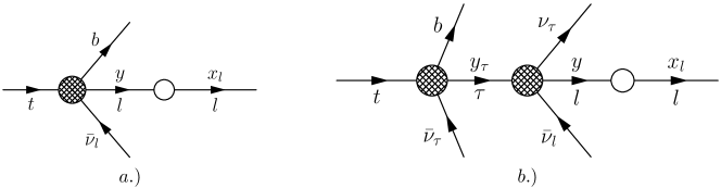
Fig. 2: Kinematics depicting the application of the structure function method, which involves factorisation of the amplitude in the ”hard sub-process” (filled circle) and the ”long-distance” contributions (empty circle) taken into account by the convolution with the structure function $D_{l}(x,\beta)$ (see (48).

The QED radiative corrected spectrum is:

$$\frac{dBr^{t\to bW^{+}\to b(e^{+}\bar{\nu}_{e})}_{Born+QED}}{dx_{e}}=\frac{1}{\Gamma_{t,RC}^{tot}}\int\limits_{x_{e}}^{1}\frac{dy_{e}}{y_{e}}D\left(\frac{x}{y_{e}},\beta_{e}\right)\frac{d\Gamma^{t\to bW^{+}\to b(e^{+}\bar{\nu}_{e})}_{B}}{dy_{e}},$$ (48)

where the structure function $D\left(x,\beta_{e}\right)$ was defined in (6).

The first order QED radiative correction reads as (using the electron energy spectrum in the Born approximation (42)):

$$\frac{dBr^{t\to bW^{+}\to b(e^{+}\bar{\nu}_{e})}_{QED_{LLA}}}{dx_{e}} = \frac{\alpha}{2\pi}\left(L_{e}-1\right)\frac{1}{\Gamma_{t,RC}^{tot}}\int\limits_{x_{e}}^{1}\frac{dy_{e}}{y_{e}}P^{(1)}\left(\frac{x_{e}}{y_{e}}\right)\frac{d\Gamma^{t\to bW^{+}\to b(e^{+}\bar{\nu}_{e})}_{B}}{dy_{e}}$$ (49)

$$= \frac{\alpha}{2\pi}\left(L_{e}-1\right)\frac{\Gamma_{t}}{\Gamma_{t,RC}^{tot}}\int\limits_{x_{e}}^{1}\frac{dy_{e}}{y_{e}}P^{(1)}\left(\frac{x_{e}}{y_{e}}\right)y_{e}\left(y_{e}^{max}-y_{e}\right)\Phi_{W}\left(y_{e}\right)$$

$$= \frac{\alpha}{2\pi}\left(L_{e}-1\right)\frac{\Gamma_{t}}{\Gamma_{t,RC}^{tot}}~{}I\left(x_{e}\right),$$

where $y_{e}^{max}=1-\eta$, and

$$I\left(x\right) = \int\limits_{x}^{1}\frac{dy}{y}P^{(1)}\left(\frac{x}{y}\right)y\left(y^{max}-y\right)\Phi_{W}\left(y\right)=$$ (50)

$$= \Phi_{W}\left(x\right)\left\{x\left(1-x\right)\left[2\ln\left(\frac{1-x}{x}\right)+\frac{3}{2}\right]+x\ln\left(x\right)+\left(1-x\right)^{2}-\frac{1}{2}\left(1-x^{2}\right)\right\}+$$

$$+ \int\limits_{x}^{1}dy\frac{\left(1-y\right)\left(y^{2}+x^{2}\right)}{y\left(y-x\right)}\left[\Phi_{W}\left(y\right)-\Phi_{W}\left(x\right)\right],$$

where $\Phi_{W}\left(x\right)$ is given in (43). The contribution of the QCD correction $\frac{dBr^{(1)}_{QCD}}{dx_{e}}$ from (44) is shown in Fig. 3, and is the same for $\ell=e,\mu,\tau$. The contributions of the QED corrections is specific to the charged lepton $e,\mu,\tau$ and shown in Fig. 3. The input parameters used in this figure and subsequently are given in a table in the Appendix. In Fig. 4, we show the electron energy spectrum in the Born approximation and compare it with the (QED + QCD) radiatively corrected ones.

It is obvious from the foregoing that the QED radiative corrections break the lepton universality, encoded at the Lagrangian level for the decays $t\to bW^{+}\to b\ell^{+}\nu_{\ell}$. It is also clear that the radiative corrections are not overall multiplicative renormalizations and they distort the Born level distributions in a non-trivial way. To quantify this, we plot the ratios $R_{e\tau}(x)$ and $R_{\mu\tau}(x)$, defined below, in Fig. 5.

$$R_{e\tau(x)} = \frac{\left(\Gamma^{t\to bW^{+}\to b(\tau^{+}\nu_{\tau})}(x=x_{\tau})\right)_{\rm Born+QCD+QED_{LLA}}}{\left(\Gamma^{t\to bW^{+}\to b(e^{+}\nu_{e})}(x=x_{e})\right)_{\rm Born+QCD+QED_{LLA}}}$$ (51)

$$R_{\mu\tau(x)}= \frac{\left(\Gamma^{t\to bW^{+}\to b(\tau^{+}\nu_{\tau})}(x=x_{\tau})\right)_{\rm Born+QCD+QED_{LLA}}}{\left(\Gamma^{t\to bW^{+}\to b(\mu^{+}\nu_{e})}(x=x_{\mu})\right)_{\rm Born+QCD+QED_{LLA}}}$$

As can be seen, the effect of the radiative corrections is very marked for the low-$x$ values of the lepton-energy spectra ($x\leq 0.3)$ and it is non-neglible also near the end-point of the spectra ($x\geq 0.7$). This is numerically an important effect and in the precision tests of the SM in the top-quark sector, which we anticipate will be carried out at the LHC, it is mandatory to take the radiative distortions of the spectra into account.

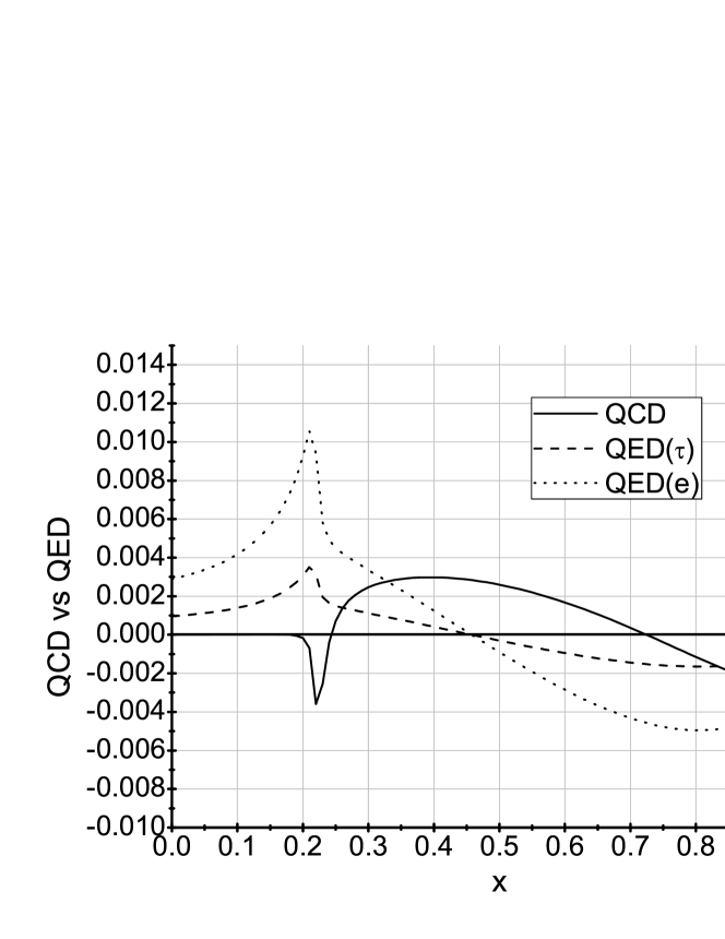
Fig. 3: QCD and QED corrections to the lepton energy spectrum in the decays $t\to bW^{+}\to b(e^{+}\nu_{e},\tau^{+}\nu_{\tau})$. The solid curve is the QCD-correction term $\frac{dBr^{(1)}_{QCD}}{dx_{e}}$ (i.e. second term from from (47)), the dashed and dotted curves are the QED-corrections $\frac{dBr^{t\to bW^{+}\to b(\tau^{+}\nu_{\tau},e^{+}\nu_{e})}_{QED_{LLA}}}{dx_{\tau,e}}$ from (49) for the $\tau^{+}$ and $e^{+}$ in the final state, respectively

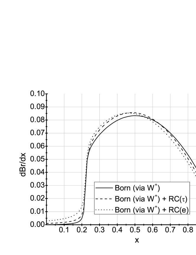
Fig. 4: Lepton energy spectra from the decays $t\to bW^{+}\to b(\ell^{+}\nu_{\ell})$ versus the lepton energy fraction $x=x_{e,\mu,\tau}$. The spectrum in the Born approximation (solid curve) is the same for $\ell^{+}=e^{+},\mu^{+},\tau^{+}$ (see (39)). The dotted curve is the $e^{+}$-energy spectrum ($dBr/dx_{e}$) including the (QCD+QED) radiative corrections for the decay $t\to bW^{+}\to b\left(e\nu_{e}\right)$ (i.e. the contributions from (47) plus the QED correction term from (49)). The dashed curve is the $\tau^{+}$-energy spectrum ($dBr/dx_{\tau}$) including the (QCD+QED) radiative corrections for the decay $t\to bW^{+}\to b\left(\tau\nu_{\tau}\right)$.

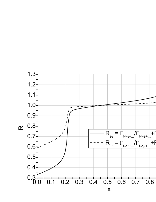
Fig. 5: Ratios of the lepton-energy spectra in the decays $t\to bW^{+}\to b(\ell^{+}\nu_{\ell})$: $R_{e\tau}(x)=\frac{d\Gamma^{t\to bW^{+}\to b\left(\tau\nu_{\tau}\right)}}{dx_{\tau}}/\frac{d\Gamma^{t\to bW^{+}\to b\left(e\nu_{e}\right)}}{dx_{e}}$ (solid curve), and $R_{\mu\tau}(x)=\frac{d\Gamma^{t\to bW^{+}\to b\left(\tau\nu_{\tau}\right)}}{dx_{\tau}}/\frac{d\Gamma^{t\to bW^{+}\to b\left(\mu\nu_{\mu}\right)}}{dx_{\mu}}$ (dashed curve), quantifying the leading order (QCD and QED) corrections to the lepton universality in semileptonic top quark decays.

V The top quark decay $t\to bH^{+}\to b(l^{+}\bar{\nu}_{l})$ in the Born approximation

Let us consider now the top quark decay induced by a charged Higgs boson:

$$t\left(p_{t}\right)\to b\left(p_{b}\right)+H^{+}\left(q\right)\to b\left(p_{b}\right)+\left(\ell^{+}\left(p_{\ell}\right)+\bar{\nu}_{\ell}\left(p_{\nu}\right)\right)$$ (52)

where we will concentrate on $\ell^{+}=\tau^{+}$ (see Fig. 1, b). Using the couplings from the Lagrangian (19) we can write the matrix element of the process (52) in the following form

$$M^{t\to bH^{+}\to b(\tau^{+}\nu_{l})}_{B} = i\frac{g^{2}V_{tb}}{8M_{W}^{2}}\frac{C}{q^{2}-M_{H}^{2}+iM_{H}\Gamma_{H}}\left[\bar{u}_{\nu_{\tau}}\left(p_{\nu}\right)\left(1+\gamma_{5}\right)u_{\tau}\left(p_{\tau}\right)\right]\times$$ (53)

$$\times \left[\bar{u}_{t}\left(p_{t}\right)\left\{A\left(1-\gamma_{5}\right)+B\left(1+\gamma_{5}\right)\right\}u_{b}\left(p_{b}\right)\right].$$

The model parameters $A$, $B$, $C$ are given in (20). Squaring this matrix element yields

$$\left|M^{t\to bH^{+}\to b(\tau^{+}\nu_{\tau})}_{B}\right|^{2}=\frac{\left(g^{2}V_{tb}\right)^{2}}{\left(q^{2}-M_{H}^{2}\right)^{2}+M_{H}^{2}\Gamma_{H}^{2}}\left(p_{t}p_{b}\right)\left(p_{\tau}p_{\nu}\right)\frac{C^{2}\left(A^{2}+B^{2}\right)}{M_{W}^{4}}.$$ (54)

Introducing the kinematic variables:

$$\begin{array}[]{lclcl}x_{\tau}=\frac{2E_{\tau}}{m_{t}},&&x_{\nu}=\frac{2E_{\nu_{\tau}}}{m_{t}},&&y=\frac{q^{2}}{m_{t}^{2}}=1+\eta-x_{b},\\ \gamma_{H}=\frac{\Gamma_{H}}{M_{H}},&&y_{0}=\frac{M_{H}^{2}}{m_{t}^{2}},&&x_{b}^{max}=1+\eta,\\ \end{array}$$ (57)

where $E_{\tau}$ and $E_{\nu_{\tau}}$ are the energies of the final $\tau$ lepton and the neutrino in the $t$-quark rest frame, respectively. $\Gamma_{H}$ is the total decay width of the charged Higgs boson, and the Breit-Wigner form of the propagator reads as

$$\frac{1}{\left|q^{2}-M_{H}^{2}+iM_{H}\Gamma_{H}\right|^{2}}=\frac{1}{\left(q^{2}-M_{H}^{2}\right)^{2}+M_{H}^{2}\Gamma_{H}^{2}}=\frac{1}{M_{H}^{4}}\frac{1}{\left(1-\frac{y}{y_{0}}\right)^{2}+\gamma_{H}^{2}}.$$ (58)

Thus the matrix element squared (54) takes the form:

$$\left|M^{t\to bH^{+}\to b(\tau^{+}\nu_{\tau})}_{B}\right|^{2}=\left(g^{2}V_{tb}\right)^{2}\frac{C^{2}\left(A^{2}+B^{2}\right)}{M_{W}^{4}}\frac{x_{b}\left(x^{max}-x_{b}\right)}{\left(1-\frac{y}{y_{0}}\right)^{2}+\gamma_{H}^{2}}\frac{1}{4y_{0}^{2}}.$$ (59)

The decay width of the unpolarised top quark decay $t\to bH^{+}\to b(\tau^{+}\bar{\nu}_{\tau})$ then takes the form:

$$\frac{d\Gamma^{t\to bH^{+}\to b(\tau^{+}\nu_{\tau})}_{B}}{dx_{b}dx_{\tau}} = \Gamma_{t}^{H}\frac{x_{b}\left(x^{max}-x_{b}\right)}{\left(1-\frac{y}{y_{0}}\right)^{2}+\gamma_{H}^{2}},$$ (60)

$$\Gamma_{t}^{H} = \frac{1}{2^{11}\pi^{3}}\left(\frac{C^{2}\left(A^{2}+B^{2}\right)}{M_{W}^{4}}\right)\left(gV_{tb}\right)^{2}\frac{m_{t}^{5}}{M_{H}^{4}}.$$ (61)

The branching ratio of this decay is:

$$\frac{dBr^{t\to bH^{+}\to b(\tau^{+}\nu_{\tau})}_{B}}{dx_{b}dx_{\tau}} = B_{t}^{H}B_{\tau}^{H}\frac{x_{b}\left(x^{max}-x_{b}\right)}{\left(1-\frac{y}{y_{0}}\right)^{2}+\gamma_{H}^{2}},\qquad B_{t}^{H}=\frac{\Gamma_{t}^{H}}{\Gamma_{t}^{tot}},$$ (62)

where $B_{\tau}^{H}$ is the branching of the decay $H^{+}\to\tau^{+}\nu_{\tau}$ Raychaudhuri:1995kv :

$$B_{\tau}^{H} = \frac{\Gamma_{H\to\tau\nu_{\tau}}}{\Gamma_{H\to\tau\nu_{\tau}}+\Gamma_{H\to c\bar{s}}}~{},$$ (63)

$$\Gamma_{H\to\tau\nu_{\tau}} = \frac{g^{2}M_{H}}{32\pi M_{W}^{2}}m_{\tau}^{2}\tan^{2}\beta,$$

$$\Gamma_{H\to c\bar{s}} = \frac{3g^{2}M_{H}}{32\pi M_{W}^{2}}\left(M_{C}^{2}\cot^{2}\beta+M_{S}^{2}\tan^{2}\beta\right).$$

For the numerical values of $\tan\beta$ that we entertain in this paper, the branching ratio $B_{\tau}^{H}=1$, to a very high accuracy. The dependence of the branching ratio of the decay $t\to bH^{+}$ on $\tan\beta$ is plotted in Fig. 6. We emphasize that in plotting this figure, radiative corrections coming from the supersymmetric sector are not included. They have been calculated in great detail in the literature, in particular for the MSSM scenario in Carena:1999py , and can be effectively incorporated by replacing the $b$-quark mass $m_{b}$ in the Lagrangian for the decay $t\to bH^{+}$ by the SUSY-corrected mass $m_{b}^{\rm corrected}=m_{b}/[1+\Delta_{b}]$. The correction $\Delta_{b}$ is a function of the supersymmetric parameters and, for given MSSM scenarios, this can be calculated using the FeynHiggs programme Hahn:2008zzd , which makes use of the results in Carena:1999py . In particular, for large values of $\tan\beta$ (say, $\tan\beta>20)$), the MSSM corrections increase the branching ratio for $t\to bH^{+}$ significantly though this is numerically not important for $\tan\beta=22$, which we use to numerically calculate the branching ratio for $t\to bH^{+}$. We emphasize that in the analysis of data in the MSSM context, the branching ratio shown here in Fig. 6 has to be corrected to include the SUSY corrections. This, for example, can be seen in a particular MSSM scenario in a recent update Sopczak:2009sm , based on the version FeynHiggs v2.6.2.

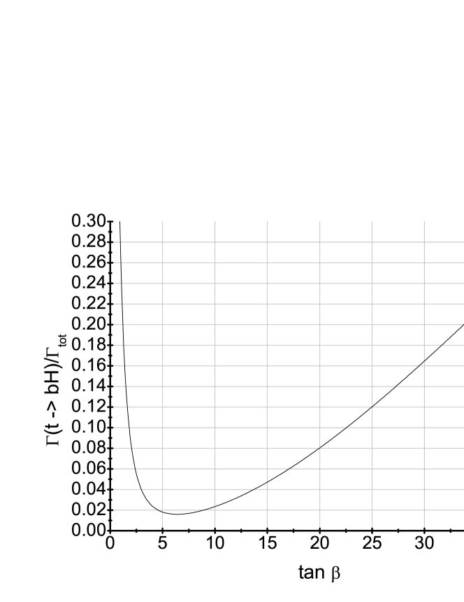
Fig. 6: Lowest order branching ratio for the decay $t\to bH^{+}$ as a function of $\tan\beta$ for $M_{H^{+}}=120$ GeV.

The lepton energy spectrum in the Born approximations has the following expression

$$\frac{dBr^{t\to bH^{+}\to b(\tau^{+}\bar{\nu}_{\tau})}_{B}}{dx_{\tau}}=\int\limits_{1-x_{\tau}}^{1}dx_{b}\frac{dBr^{t\to bH^{+}\to b(\tau^{+}\nu_{\tau})}_{B}}{dx_{b}dx_{\tau}}=B_{t}^{H}B_{\tau}^{H}\cdot\Phi_{H}\left(x_{\tau}\right),$$ (64)

where

$$\Phi_{H}\left(x\right) = \int\limits_{0}^{x}dy\frac{y\left(1-y\right)}{\left(1-\frac{y}{y_{0}}\right)^{2}+\gamma^{2}}$$ (65)

$$= y_{0}^{2}\left\{\frac{1-y_{0}}{\gamma_{H}}\left[\arctan\left(\frac{1}{\gamma_{H}}\right)+\arctan\left(\frac{x-y_{0}}{y_{0}\gamma}\right)\right]\right.+$$

$$+ \left.\left(2y_{0}-1\right)\ln\left(\frac{y_{0}}{y_{0}-x}\right)-x\right\}.$$

V.1 QCD radiative corrections

The leading order QCD corrections to the decay $t\to bH^{+}\to b(\tau^{+}\nu_{\tau})$ is calculated in a similar way as for the case of $t\to bW^{+}\to b(\tau^{+}\nu_{\tau})$. The derivations for the Dalitz distribution $dBr/dx_{b}dx_{\tau}$ and the $\tau$-energy spectrum $dBr/dx_{\tau}$ are given in Appendix B.

V.2 QED radiative corrections in the leading logarithmic approximation

To calculate the QED radiative corrections in the leading logarithmic approximation we will again use the structure function method, which gives:

$$\frac{dBr^{t\to bH^{+}\to b(\tau^{+}\nu_{\tau})}_{Born+QED}}{dx_{\tau}}=\frac{B_{\tau}^{H}}{\Gamma_{t,RC}^{tot}}\int\limits_{x_{\tau}}^{1}\frac{dy}{y}D\left(\frac{x_{\tau}}{y},\beta_{\tau}\right)\frac{d\Gamma^{t\to bH^{+}\to b(\tau^{+}\nu_{\tau})}_{B}}{dy}.$$ (66)

where the large QED logarithm now is $\beta_{\tau}$ (see (3)). The first order QED radiative correction reads as

$$\frac{dBr^{t\to bH^{+}\to b(l^{+}\nu_{l})}_{QED_{LL}}}{dx_{l}} = \frac{\alpha}{2\pi}\left(L_{l}-1\right)\frac{B_{\tau}^{H}}{\Gamma_{t,RC}^{tot}}\int\limits_{x_{l}}^{1}\frac{dy}{y}P^{(1)}\left(\frac{x_{l}}{y}\right)\frac{d\Gamma^{t\to bH^{+}\to b(l^{+}\nu_{l})}_{B}}{dy}$$ (67)

$$= \frac{\alpha}{2\pi}\left(L_{l}-1\right)\frac{\Gamma_{t}^{H}}{\Gamma_{t,RC}^{tot}}B_{\tau}^{H}\int\limits_{x_{l}}^{1}\frac{dy}{y}P^{(1)}\left(\frac{x_{l}}{y}\right)\Phi_{H}\left(y_{l}\right)$$

$$= \frac{\alpha}{2\pi}\left(L_{l}-1\right)\frac{\Gamma_{t}^{H}}{\Gamma_{t,RC}^{tot}}B_{\tau}^{H}I_{H}\left(x_{l}\right),$$

where $\Phi_{H}\left(x\right)$ is the Born spectrum defined in (65) and

$$I_{H}\left(x\right) = \int\limits_{x}^{1}\frac{dy}{y}P^{(1)}\left(\frac{x}{y}\right)\Phi_{H}\left(y\right)$$ (68)

$$= \Phi_{H}\left(x\right)\left\{x+\frac{1}{2}+\ln\left(x\right)+2\ln\left(\frac{1-x}{x}\right)\right\}$$

$$+ \int\limits_{x}^{1}dy\frac{\left(y^{2}+x^{2}\right)}{y^{2}\left(y-x\right)}\left[\Phi_{H}\left(y\right)-\Phi_{H}\left(x\right)\right].$$

The contribution of the QED corrections (67) is shown in Fig. 7 and compared with the QCD corrections from (104).

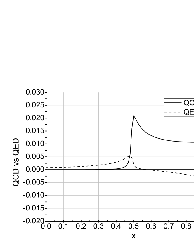
Fig. 7: QCD and QED corrections to the lepton energy spectrum in the decays $t\to bH^{+}\to b\tau^{+}\nu_{\tau}$. The solid curve is the QCD corrections, i.e. the second term on the r.h.s. of the first line of Eq. (105) divided by the total decay width $\Gamma_{t,RC}^{tot}$, and the dashed curve is the QED corrections $\frac{dBr^{t\to bH^{+}\to b\tau^{+}\nu_{\tau}}_{QED_{LLA}}}{dx_{\tau}}$ from Eq. (67) for the $\tau^{+}$ in the final state.

In Fig. 8 we show the lepton energy spectrum in the Born approximation and compare it with the radiatively corrected one.

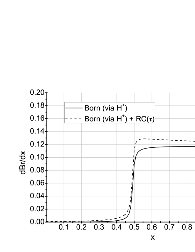
Fig. 8: Lepton energy spectra from the decays $t\to bH^{+}\to b(\tau^{+}\nu_{\tau})$ versus the $\tau$ energy fraction $x=x_{\tau}$ for $M_{H^{+}}=120$ GeV and $\tan\beta=22$. The solid curve shows the Born spectrum (see (64)) and the dashed curve is the spectrum including the (QED + QCD) radiative corrections from Fig. 7 (i.e. QCD corrections are taken from Eq. (105) and the QED corrections are taken from (67)).

Contrasting the $\tau$-energy spectra in this figure with the corresponding spectra in Fig. 4 shows that the $\tau$-leptons from the decay $t\to bH^{+}\to b\tau^{+}\nu_{\tau}$ are distinctly more energetic. This feature is well known in the literature. We have calculated here the (QCD + QED) corrections to these spectra and checked their perturbative stability.

VI Top decay channels involving the $\tau$ lepton

The radiatively corrected charged lepton energy spectra from the decays $t\to bW^{+}\to b\ell^{+}\nu_{\ell}$ (for $\ell^{+}=e^{+},\mu^{+},\tau^{+}$) and $t\to bH^{+}\to b(\tau^{+}\nu_{\tau})$ presented here will be helpful in undertaking precision tests of the SM and in the searches for the $H^{\pm}$-induced effects in the semileptonic decays of the top quark. Integrating these spectra from some experimental threshold lepton energy, the anticipated enhancement in the branching ratio for the $t\to b(\tau^{+}\nu_{\tau})$ mode over the other two semileptonic modes $t\to b(\mu+\nu_{\mu},e^{+}\nu_{e})$ provides the experimental handle on the $H^{\pm}$ searches. This is the strategy which is being used at the Tevatron, where searches have also been made in the decays $H^{+}\to c\bar{s}$ (and in the charge conjugate modes), but this final state is of interest only in the region $\tan\beta<1$, which we do not entertain here. However, as already mentioned in the introduction, the characteristic polarisation of the $\tau^{\pm}$ produced in the decays $W^{\pm}\to\tau^{\pm}\nu_{\tau}$ and $H^{\pm}\to\tau^{\pm}\nu_{\tau}$, which reflects itself in the energy distributions of the $\tau^{\pm}$-decay products, can be used to discriminate the $W^{\pm}$-induced and $H^{\pm}$-induced final states. In this section, we calculate the energy spectra of the so-called single charged-prong events in $\tau$-decays. The $\tau^{\pm}$-polarisation effects on the $\tau^{\pm}$ decay products have already been investigated in the literature, in particular in Bullock:1992yt ; Raychaudhuri:1995cc , which we shall make use of, convoluting these spectra with the $\tau^{+}$-energy spectrum from the decay chain $t\to b(W^{+},H^{+})\to b(\tau^{+}\nu_{\tau})$ calculated by us here. To that end, we consider the following $\tau^{\pm}$ decay chains

$$t \to b(W^{+},H^{+})\tau\bar{\nu}_{\tau}\to jet(b)+\bar{\nu}_{\tau}+\nu_{\tau}+\bar{\nu}_{l}+l,\qquad l=e^{+},\mu^{+};$$ (69)

$$t \to b(W^{+},H^{+})\tau\bar{\nu}_{\tau}\to jet(b)+\bar{\nu}_{\tau}+\nu_{\tau}+\pi^{+};$$

$$t \to b(W^{+},H^{+})\tau\bar{\nu}_{\tau}\to jet(b)+\bar{\nu}_{\tau}+\nu_{\tau}+\pi^{+}+\pi^{0};$$

$$t \to b(W^{+},H^{+})\tau\bar{\nu}_{\tau}\to jet(b)+\bar{\nu}_{\tau}+\nu_{\tau}+\pi^{+}+2\pi^{0};$$

$$t \to b(W^{+},H^{+})\tau\bar{\nu}_{\tau}\to jet(b)+\bar{\nu}_{\tau}+\nu_{\tau}+2\pi^{+}+\pi^{-},$$

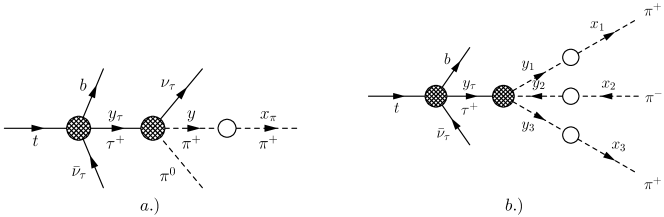
Fig. 11: Kinematics of the Structure Function method for the decay a) $t\to b\bar{\nu}_{\tau}\nu_{\tau}\pi^{0}\pi^{+}$ and b) $t\to b\bar{\nu}_{\tau}\nu_{\tau}\pi^{+}\pi^{-}\pi^{+}$, involving a $\pi^{+}$ in the final state.

involving the leptons $e^{+}$, $\mu^{+}$, the $\pi^{+}$, the vector and the axial-vector mesons $\rho^{+}$ and $a_{1}^{+}$, respectively, with the subsequent decays of the $\rho^{+}$ and $a_{1}^{+}$, as indicated. Keeping in mind the long-distance nature of the QED interactions, providing the ”large logarithms”, one must include the structure function associated factors only with the final charged particles-leptons or pions (see Fig. 2, b and Fig. 11, a, b). In the rest frame of the top quark, the $\tau$-leptons from the decays $t\to b(W^{+},H^{+})\to b(\tau^{+}\nu_{\tau})$ have much larger energy and 3-momentum compared to the$\tau$- mass, i.e. $E_{\tau}\gg m_{\tau}$. The energy spectrum of the $\tau$-lepton decay products must be modified to take this into account Bullock:1992yt . For example for the decay $\tau\to\mu\nu\nu$ of the $\tau$-lepton with energy $E_{\tau}$, the $E_{\mu}$-energy spectrum can be obtained from (15) (see also Eq. (2.8) in Bullock:1992yt ):

$$\frac{dBr_{B}^{\tau\to\mu\nu\nu}}{dz} = \int d\cos\theta\int\limits_{z}^{1}\frac{dBr_{B}}{d\cos\theta dx}\delta\left(z-\frac{x}{2}\left(1-\cos\theta\right)\right)dx$$ (70)

$$= \Phi_{l}\left(z\right)=\frac{B_{l}}{3}\left(1-z\right)\left[5+5z-4z^{2}-P_{\tau}\left(1+z-8z^{2}\right)\right],$$

where $z$ is the energy fraction of the $\mu$ in the indicated decay:

$$z=\frac{E_{a}}{E_{\tau}}=\frac{x}{2}(1-\cos\theta)=\frac{x_{a}}{x_{\tau}},$$ (71)

$x=2E_{\mu}/m_{\tau}$, and $\theta$ is the angle between the directions of the $\tau$ and the $\mu$ 3-momenta. The index $a$ in $E_{a}$ shows the final particle involved. Here, $a=\mu$ (the expression above holds also for the $e^{+}$-energy spectrum). We also need the energy spectra for other particles in the $\tau$-lepton decay, i.e. for $a=\pi^{+},\rho,a_{1}$. The corresponding distributions were obtained in Bullock:1992yt : for $\Phi_{\pi}\left(z\right)$ see Eq. (2.4) and for $\Phi_{\rho,a_{1}}\left(z\right)$ see Eq. (2.22) in the cited paper.

VI.1 Leptons in final state

For the $\tau^{+}$-decay with the leptons in the final state (i.e. $a=e^{+},\mu^{+}$), the final expression for the lepton energy spectrum in the Born approximation is

$$\frac{dBr^{t\to b+\bar{\nu}_{\tau}+\nu_{\tau}+\nu_{l}+\ell^{+}}_{B}}{dx_{\ell}}=\int\limits_{x_{l}}^{1}\frac{dy_{\tau}}{y_{\tau}}\frac{dBr^{t\to b(\tau^{+}\nu_{\tau})}_{\rm Born}}{dy_{\tau}}\Phi_{l}\left(\frac{x_{l}}{y_{\tau}}\right)$$ (72)

where the $t$-quark decay width $\frac{dBr^{t\to b(\tau^{+}\nu_{\tau})}_{\rm Born}}{dx_{\tau}}$ is taken from (42) or (64) and $\Phi_{l}\left(z\right)$ was defined in (70). To take into account the QED radiative corrections in LLA we again use the SF approach illustrated in Section II (see formula (II) and Fig. 2, b). The radiatively corrected spectrum is then given by

$$\frac{dBr^{t\to b+\bar{\nu}_{\tau}+\nu_{\tau}+\nu_{\ell}+\ell^{+}}_{QED_{LLA}+QCD}}{dx_{l}} = \frac{\left\{1,B_{\tau}^{H}\right\}}{\Gamma_{t,RC}^{tot}}\int\limits_{x_{l}}^{1}\frac{dy}{y}D_{l}\left(\frac{x_{l}}{y},\beta_{l}\right)\int\limits_{2\sqrt{\eta}}^{1}dx_{b}\times$$ (73)

$$\times \frac{d\Gamma^{t\to b+\bar{\nu}_{\tau}+\nu_{\tau}+\nu_{\ell}+\ell^{+}}_{\rm Born}}{dx_{b}dy}\left(1-\frac{\alpha_{s}}{\pi}\left\{\frac{2}{3}\frac{F_{W}\left(y,x_{b}\right)}{y\left(y^{max}-y\right)},F_{H}\left(y,x_{b}\right)\right\}\right),$$

where the first entry in the curly braces is for the decay channels which go via the $W^{+}b$ intermediate state, and the second entry is for the decays which go via the intermediate state $H^{+}b$. The function $F_{W}\left(x_{l},x_{b}\right)$ represents the non-leading contributions of the QCD corrections and was defined in (46). The definition of the function $F_{H}\left(x_{l},x_{b}\right)$ is given in (105). The differential branching ratios from the decay chain $t\to bW^{+}\to b(\tau^{+}\to\mu^{+}\nu_{\mu}\bar{\nu}_{\tau})\nu_{\tau}$ are shown in Fig. 9 and from the decay chain $t\to bH^{+}\to b(\tau^{+}\to\mu^{+}\nu_{\mu}\bar{\nu}_{\tau})\nu_{\tau}$ in Fig. 10.

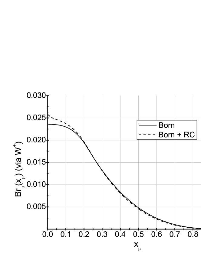
Fig. 9: Differential branching ratio $\frac{dBr^{t\to bW^{+}\to b((\tau^{+}\to\mu^{+}\nu_{\mu}\bar{\nu}_{\tau})\nu_{\tau}}_{B}}{dx_{\mu}}$ (see (72)) as a function of the $\mu^{+}$ energy fraction $x_{\mu}$ in the Born approximation (solid curve) and with the QED and QCD radiative corrections (dashed curve) (see (73)).

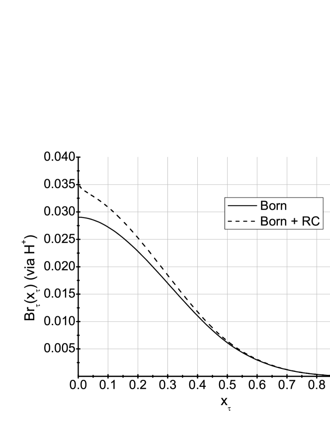
Fig. 10: Differential branching ratio $\frac{dBr^{t\to bH^{+}\to b((\tau^{+}\to\mu^{+}\nu_{\mu}\bar{\nu}_{\tau})\nu_{\tau}}_{B}}{dx_{\mu}}$ as a function of the $\mu^{+}$ energy fraction $x_{\mu}$ in the Born approximation (solid curve) and with the QED and QCD radiative corrections (dashed curve), involving the $bH^{+}$ intermediate state.

VI.2 Hadrons in the final state

In this case, we have to take into account the decay chain involving the final decays $\tau^{+}\to(\pi^{+},\rho^{+},a_{1}^{+})\nu_{\tau}$ with the subsequent decays of the $\rho^{+}$- and the $a_{1}^{+}$-mesons into pions. The $\tau$-energy spectrum is already given above. Consider first the decay $\tau^{+}\to\rho^{+}\bar{\nu}_{\tau}$, in which case the $\rho^{+}$-energy spectrum is given by

$$\frac{dBr^{t\to b+\nu_{\tau}+(\tau^{+}\to\rho^{+}+\bar{\nu}_{\tau})}_{B}}{dx_{\rho}} = \int\limits_{x_{\rho}}^{1}\frac{dx_{\tau}}{x_{\tau}}\frac{dBr^{t\to b+\bar{\nu}_{\tau}+\tau}_{B}}{dx_{\tau}}\Phi_{\rho}\left(\frac{x_{\rho}}{x_{\tau}}\right),$$ (74)

where the function $\Phi_{\rho}(x)$ describes the conversion of the energetic $\tau$-lepton into the energetic $\rho$-meson. This function was calculated in Ref. Bullock:1992yt , which we incorporated in our numerical calculations. The distribution in the pion energy fraction $x_{\pi}$ resulting from the $\rho^{+}\to\pi^{+}\pi^{0}$ decay takes the form:

$$\frac{dBr^{t\to b+\nu_{\tau}+(\tau\to\bar{\nu}_{\tau}+(\rho\to\pi^{+}\dots))}_{\rm Born}}{dx_{\pi}} = \int\limits_{x_{\pi}}^{1}\frac{dx_{\rho}}{x_{\rho}}\frac{dBr^{t\to b+\nu_{\tau}+(\tau\to\rho+\bar{\nu}_{\tau})}_{\rm Born}}{dx_{\rho}}R_{\rho}\left(\frac{x_{\pi}}{x_{\rho}}\right),$$ (75)

where the function $R_{\rho}(x)$ describes the conversion of the energetic $\rho$ meson into energetic pions (i.e. $\rho^{\pm}\to\pi^{\pm}\pi^{0}$):

$$R_{\rho}\left(x\right)=\frac{1}{\Gamma}\frac{d\Gamma}{dx},\qquad x=\frac{E_{\pi^{\pm}}}{E_{\rho}}=\frac{x_{\pi^{\pm}}}{x_{\rho}},$$ (76)

This function was investigated in Raychaudhuri:1995cc (see Fig. 1 in Raychaudhuri:1995cc ).

The radiative corrections (”large distance contributions”) can be obtained by using the structure function approach as:

$$\frac{dBr^{t\to b+\nu_{\tau}+(\tau\to\bar{\nu}_{\tau}+(\rho\to\pi^{+}\dots))}_{RC}}{dx_{\pi}} = \frac{\left\{1,B_{\tau}^{H}\right\}}{\Gamma_{t,RC}^{tot}}\int\limits_{x_{\pi}}^{1}\frac{dy_{\pi}}{y_{\pi}}\times$$ (77)

$$\times \frac{d\Gamma^{t\to b+\nu_{\tau}+(\tau\to\bar{\nu}_{\tau}+(\rho\to\pi^{+}\dots))}_{\rm Born}}{dy_{\pi}}D_{\pi}\left(\frac{x_{\pi}}{y_{\pi}},\beta_{\pi}\right),$$

where $D_{\pi}(z)$ is the structure function of the charged pion Kuraev:2006yq :

$$D_{\pi}\left(x,\beta_{\pi}\right) = \delta\left(1-x\right)+\beta P_{\pi}^{(1)}\left(x\right)+\frac{1}{2!}\beta^{2}P_{\pi}^{(2)}\left(x\right)+\cdots,$$ (78)

$$\beta_{\pi} = \frac{\alpha}{2\pi}\left(\ln\frac{m_{t}^{2}}{M_{\pi}^{2}}-1\right),$$

and the quantities $P_{\pi}^{(n)}\left(x\right)$ have the form:

$$P_{\pi}^{(1)}\left(x\right) = \left(\frac{2x}{1-x}\right)_{+}=\lim_{\Delta\to 0}\left[\frac{2x}{1-x}\theta\left(1-x-\Delta\right)+\left(2\ln\left(\Delta\right)+2\right)\delta\left(1-x\right)\right],$$ (79)

The formula similar to (68) in the case of pions reads as:

$$\int\limits_{x}^{1}\frac{dy}{y}P_{\pi}^{(1)}\left(\frac{x}{y}\right)\phi\left(y\right) = \phi\left(x\right)\left\{2\ln\left(1-x\right)+2\right\}+\int\limits_{x}^{1}\frac{dy}{y}\frac{2x}{y-x}\left[\phi\left(y\right)-\phi\left(x\right)\right],$$ (80)

where $\phi(x)$ is any arbitrary function we want to convolute with the structure function $D_{\pi}\left(x,\beta_{\pi}\right)$ in the leading order perturbation theory. The smoothed form of the structure function $D_{\pi}\left(x,\beta_{\pi}\right)$ takes the form:

$$D_{\pi}\left(x,\beta_{\pi}\right)=2\beta_{\pi}\left(1-z\right)^{2\beta_{\pi}-1}\left(1+\beta_{\pi}\right)-\beta_{\pi}+O\left(\beta_{\pi}^{2}\right).$$ (81)

The energy distribution of the charged pion obtaining from the decay $a_{1}^{+}\to\pi^{+}...$ from the parent $\tau$ decay can be derived analogously.

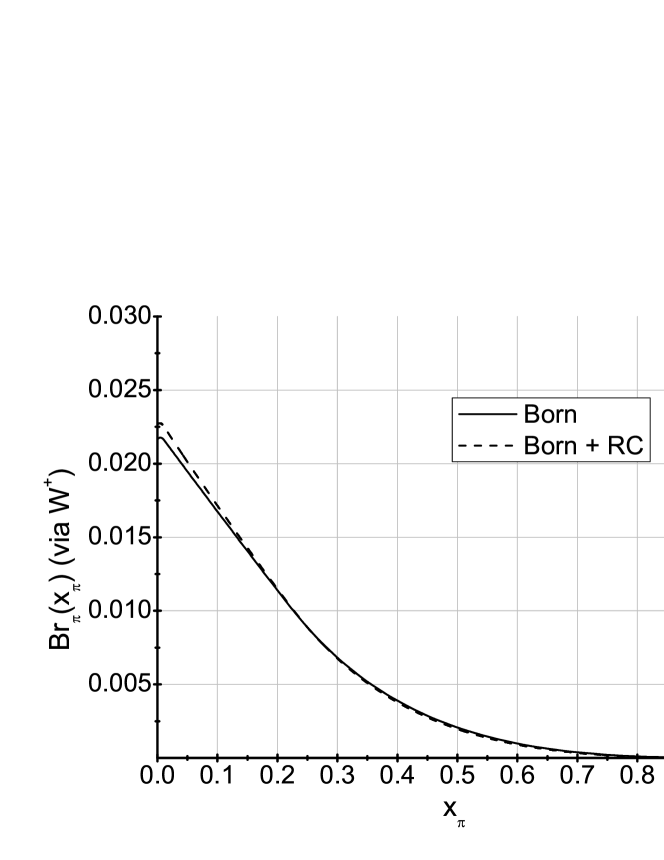
Fig. 12: Differential branching ratio $\frac{dBr^{t\to bW^{+}\to b((\tau^{+}\to\pi^{+}\bar{\nu}_{\tau})\nu_{\tau}}_{B}}{dx_{\pi}}$ (see (72) as a function of the $\pi^{+}$ energy fraction $x_{\pi}$ in the Born approximation (solid curve) and with the QED and QCD radiative corrections taken into account (dashed curve) (see (73)).

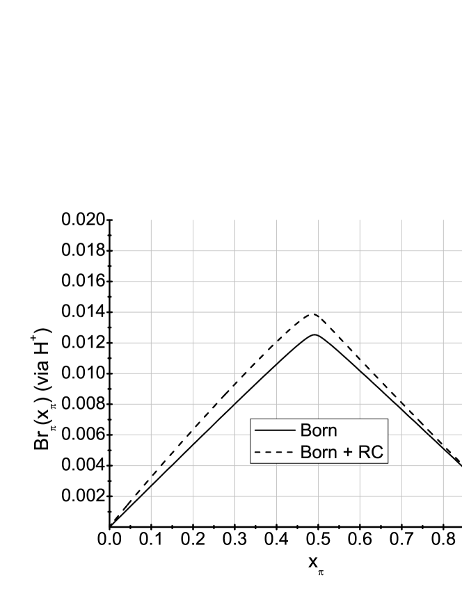
Fig. 13: Differential branching ratio $\frac{dBr^{t\to bH^{+}\to b((\tau^{+}\to\pi^{+}\bar{\nu}_{\tau})\nu_{\tau}}_{B}}{dx_{\pi}}$ as a function of the $\pi^{+}$ energy fraction $x_{\pi}$ in the Born approximation (solid curve), and with the QED and QCD radiative corrections taken into account (dashed curve), involving the $bH^{+}$ intermediate state.

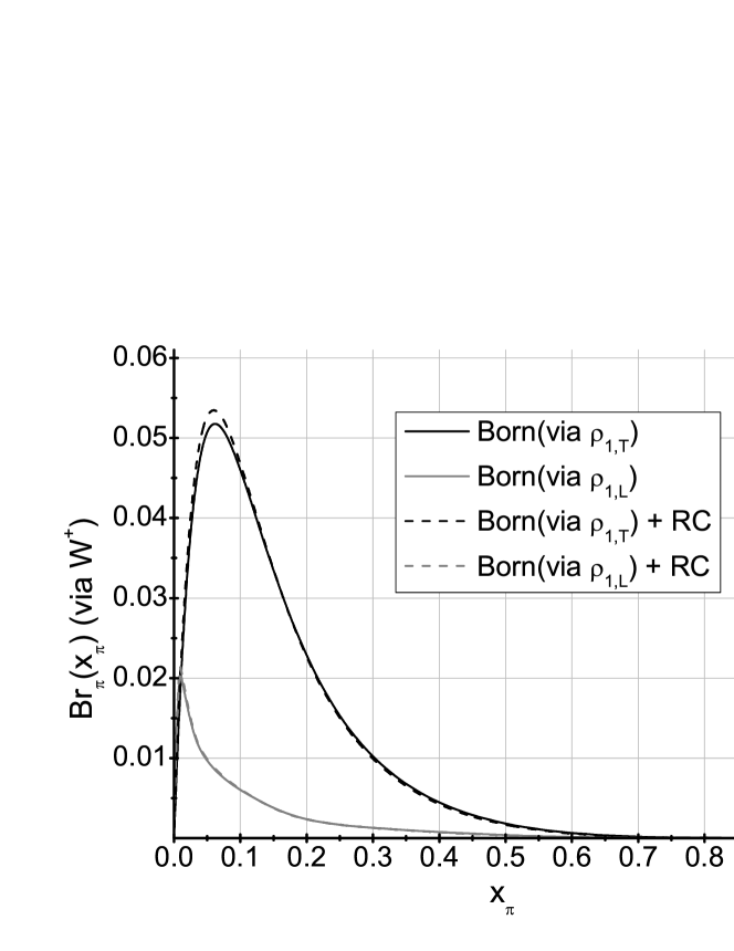
Fig. 14: Differential branching ratio $\frac{dBr^{t\to bW^{+}\to b((\rho^{+}\to\pi^{+}\pi^{0})\bar{\nu}_{\tau})}_{B}}{dx_{\pi}}$ as a function of the pion energy fraction $x_{\pi}$ in the Born approximation (solid curves) and including the QED and QCD radiative corrections (dashed curves). The upper curves are for the transverse polarisation of the $\rho$ and the lower curves correspond to the case where the $\rho$ is longitudinally polarised.

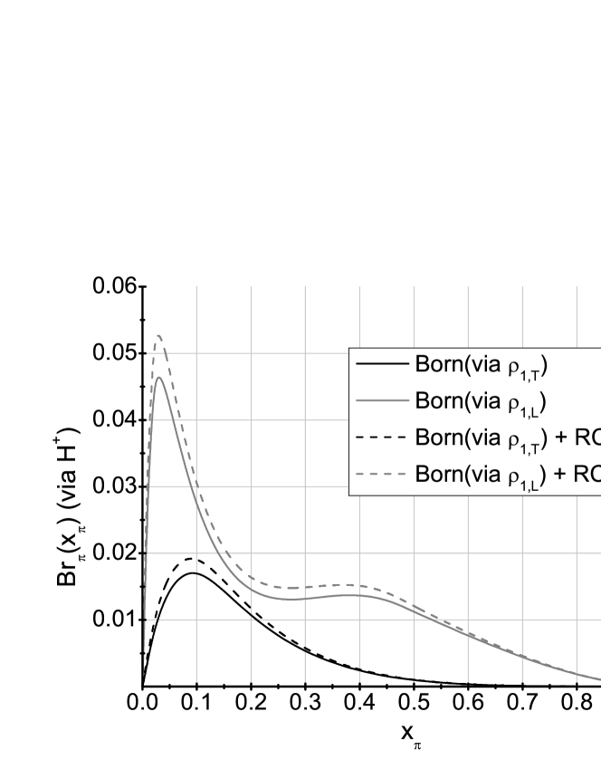
Fig. 15: Differential branching ratio $\frac{dBr^{t\to bH^{+}\to b((\rho^{+}\to\pi^{+}\pi^{0})\bar{\nu}_{\tau})}_{B}}{dx_{\pi}}$ as a function of the pion energy fraction $x_{\pi}$ in the Born approximation (solid curves) and including the QED and QCD radiative corrections (dashed curves), involving the $bH^{+}$ intermediate state. The upper curves are for the longitudinal polarisation of the $\rho$ and the lower curves correspond to the case where the $\rho$ is transversely polarised.

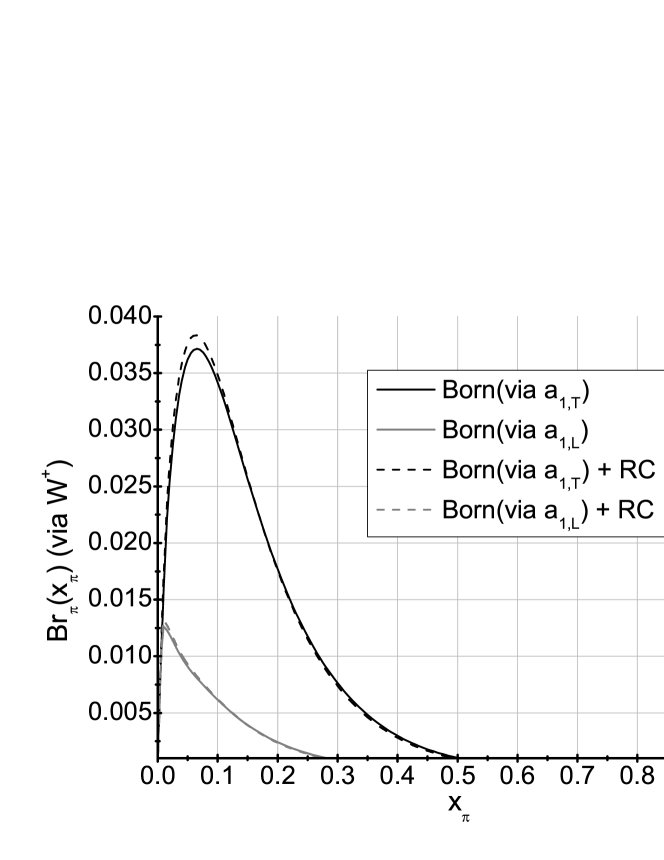
Fig. 16: Differential branching ratio $\frac{dBr^{t\to bW^{+}\to b((a_{1}^{+}\to(3\pi)^{+})\bar{\nu}_{\tau})}_{B}}{dx_{\pi}}$ as a function of the pion energy fraction $x_{\pi}$ in the Born approximation (solid curves) and including the QED and QCD radiative corrections (dashed curves). The upper curves are for the transverse polarisation of the $a_{1}$ and the lower curves correspond to the case where the $a_{1}$ is longitudinally polarised.

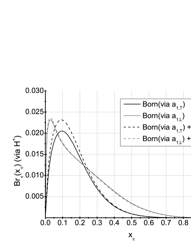
Fig. 17: Differential branching ratio $\frac{dBr^{t\to bH^{+}\to b((a_{1}^{+}\to(3\pi)^{+})\bar{\nu}_{\tau})}_{B}}{dx_{\pi}}$ as a function of the pion energy fraction $x_{\pi}$ in the Born approximation (solid curves) and including the QED and QCD radiative corrections (dashed curves), involving the $bH^{+}$ intermediate state. The polarisation of the $a_{1}^{+}$ is indicated in the figure.

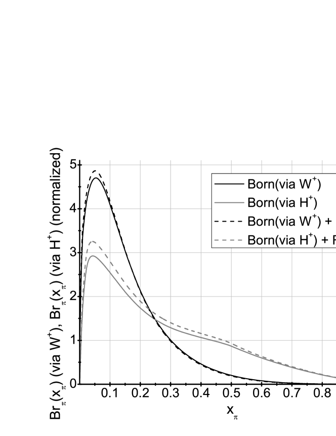
Fig. 18: Normalised inclusive pion energy spectra from the decays $t\to b(W^{+},H^{+})\to b(\pi^{+}+X)\bar{\nu}_{\tau}$ as a function of the pion energy fraction $x_{\pi}$ in the Born approximation (solid curves) and including the QED and QCD radiative corrections (dashed curves).

VII Summary

In the first part of our paper, we have calculated the QCD and QED radiative corrections to the semileptonic decays $t\to bW^{+}\to b\ell^{+}\nu_{\ell}$ $(\ell=e,\mu,\tau)$ in the SM. Of particular interest are the charged lepton energy spectra, which we have calculated using the SF approach to resum the leading order (in QED) and leading and next-to-leading order (in QCD) contributions. These spectra will be measured accurately at the LHC and will be crucial to check the lepton ($e,\mu,\tau$) universality in the semileptonic decays of the top quarks in SM. In doing this, it will be crucial to take into account the QED and QCD radiative corrections in the energy spectra. The numerical extent of such corrections is shown in Fig. 5 for the ratios $R_{e\tau}$ and $R_{\mu\tau}$, which is one of our principal results in this paper. The rest of our paper is addressed to the possible effects of a charged Higgs boson $H^{\pm}$ with $M_{H^{\pm}}<m_{t}-m_{b}$ in the semileptonic decays of the top quark. To avoid the constraints on $M_{H^{\pm}}$ coming from the $B\to X_{s}\gamma$ decay, we assume that the Higgs sector is part of a supersymmetric theory. Except for the SUSY radiative corrections, which can be effectively taken into account by the supersymmetric renormalisation of the $b$-quark mass, there are no other effects of the supersymmetric sector on the decay widths and distributions. We have considered only the large-$\tan\beta$ parameter space of this model, in which case the decays of the $H^{\pm}$ are dominated by the final state $H^{\pm}\to\tau^{\pm}\nu_{\tau}$. In Figs. 4 and 8, we have contrasted the Born and radiatively corrected $\tau$-lepton energy spectra from the decays $t\to b(W^{+},H^{+})\to\tau^{+}\nu_{\tau}$ for a specific choice of the parameters $M_{H^{\pm}}=120$ GeV and $\tan\beta=22$. While the Born level spectra are well documented in the literature, effects of the radiative corrections on the spectra are, to the best of our knowledge, new results.

The contribution of an $H^{\pm}$ in $t$ ($\bar{t}$) decays, if allowed kinematically, will enhance the decay rate for $t\to b\tau^{+}\nu_{\tau}$ ($\bar{t}\to\bar{b}\tau^{-}\bar{\nu}_{\tau}$), which is the main $H^{\pm}$-search strategy at the Tevatron. However, with a much larger $t\bar{t}$ cross section and the luminosity anticipated at the LHC, this search strategy can be further strengthened by taking into account the different $\tau^{\pm}$-polarisations in the decays $W^{\pm}\to\tau^{\pm}\nu_{\tau}$ and $H^{\pm}\to\tau^{\pm}\nu_{\tau}$. As the polarisation information of the $\tau^{\pm}$ is transmitted to the decay products of the $\tau^{\pm}$, we have calculated the energy distributions of the charged particles ($e^{\pm},\mu^{\pm},\pi^{\pm},\rho^{\pm},a_{1}^{\pm}$) in the single-charge-prong decays of the $\tau^{\pm}$, as well as the inclusive charged pion spectra from the decay chains $t\to b(W^{\pm},H^{\pm})\to b(\tau^{\pm},\nu_{\tau})\to b\pi^{\pm}+X$. The results at the Born level are well known in the literature. We have calculated the perturbative stability of these distributions. The entire effects of the radiative corrections presented here can be implemented in existing Monte Carlos, such as PYTHIA and HERWIG, to provide an improved theoretical profile of the semileptonic decays of the top quark in the SM and can be combined with FeynHiggs to include the SUSY-related corrections specific to particular MSSM scenarios.

Acknowledgments

The work presented here is partially supported by the Heisenberg-Landau Program. We thank Gustav Kramer for reading the manuscript and helpful comments, and Sven Moch for communication on the top quark production cross section at the LHC.

Appendix A Numerical values of the input parameters

For our numerical calculations we used the following values of the parameters:

Parameter	Value	Parameter	Value	Parameter	Value
$\alpha^{-1}$	$137.035999679$	$m_{t}$	$171.2~{}\mbox{GeV}$	$\tan\beta$	$40$
$\alpha_{s}$	$0.1176$	$m_{b}$	$4.20~{}\mbox{GeV}$	$Br\left(\tau\to\mu\nu_{\tau}\bar{\nu}_{\mu}\right)$	$17.36\times 10^{-2}$
$m_{e}$	$0.510998910~{}\mbox{MeV}$	$M_{\pi}$	$0.13957018~{}\mbox{GeV}$	$Br\left(\tau\to\pi\nu_{\tau}\right)$	$10.91\times 10^{-2}$
$m_{\mu}$	$105.6583668~{}\mbox{MeV}$	$M_{\rho}$	$0.775~{}\mbox{GeV}$	$Br\left(\tau\to\rho\nu_{\tau}\right)$	$25.52\times 10^{-2}$
$m_{\tau}$	$1.77684~{}\mbox{GeV}$	$\Gamma_{\rho}$	$0.1462~{}\mbox{GeV}$	$Br\left(\tau\to a_{1}\nu_{\tau}\right)$	$1.859\times 10^{-1}$
$M_{W}$	$80.398~{}\mbox{GeV}$	$M_{a_{1}}$	$1.230~{}\mbox{GeV}$
$\Gamma_{W}$	$2.141~{}\mbox{GeV}$	$\Gamma_{a_{1}}$	$0.420~{}\mbox{GeV}$
$M_{H}$	$120~{}\mbox{GeV}$	$G_{F}$	$1.16637\times 10^{-5}~{}\mbox{GeV}^{-2}$
$\Gamma_{H}$	$2~{}\mbox{GeV}$	$g$	$0.653057$

Appendix B Radiative corrections to top quark decay via charged Higgs

Here we give details of the QCD radiative corrections to the width of $t$-quark decay $t(p)\to b(p_{b})+\tau(p_{\tau})+\bar{\nu}(p_{\nu})$ with the charged Higgs boson in the intermediate state.

The lowest order QCD corrections can be calculated in a similar way as in QED and in the final result one must do the replacements

$$\alpha\to\alpha_{s}C_{F},\qquad C_{F}=\frac{N_{c}^{2}-1}{2N_{c}}=\frac{4}{3},$$ (82)

where $N_{c}=3$ is the number of quark colours.

We start from the counter-terms associated with the $t$ and $b$ quarks. Taking them into account yields a multiplicative renormalisation factor in the expression for the differential width

$$d\Gamma\to d\Gamma Z_{bt},$$ (83)

$$Z_{bt}=1-\frac{\alpha}{2\pi}\left[\ln\frac{\Lambda^{2}}{m_{t}^{2}}+\frac{3}{2}\ln\frac{m_{t}^{2}}{m_{b}^{2}}+\frac{9}{2}-2\ln\frac{m_{t}^{2}}{\lambda^{2}}\right],$$ (84)

where $m_{t}$ and $m_{b}$ are the masses of top and bottom quark. The auxiliary parameters $\Lambda$ and $\lambda$ are introduced to regularise the ultraviolet (UV) and infrared (IR) singularities, respectively. Sometimes $\lambda$ is also dubbed as a fictitious ”photon (gluon) mass”. The dependence of the decay width on these parameters will disappear from the final result. The UV-cutoff $\Lambda$ will be absorbed by the coupling constant renormalisation and the IR-cutoff $\lambda$ will be cancelled by taking into account the emission of the virtual and real gluons.

Virtual corrections associated with the vertex type Feynman diagram require the calculation of the following integral involving the loop 4-momentum

$$V=\int\frac{d^{4}k}{i\pi^{2}}\frac{\gamma_{\mu}(\hat{p}_{b}-\hat{k}+m_{b})(\hat{p}-\hat{k}+m_{t})\gamma^{\mu}}{(k^{2}-\lambda^{2})((p_{b}-k)^{2}-m_{b}^{2})((p-k)^{2}-m_{t}^{2})}.$$ (85)

Using the Feynman prescription of combining the denominators and performing the loop momentum integration (here we must impose the ultraviolet cut-off) we arrive at

$$V=4\ln\frac{\Lambda^{2}}{m_{t}m_{b}}-2\left(pp_{b}\right)\int\limits_{0}^{1}\frac{dx}{p_{x}^{2}}\ln\frac{p_{x}^{2}}{\lambda^{2}}-2\left(m_{t}+m_{b}\right)\int\limits_{0}^{1}\frac{dx}{p_{x}^{2}}\left(xm_{b}+(1-x)m_{t}\right),$$ (86)

with $p_{x}^{2}=x^{2}m_{b}^{2}+(1-x)^{2}m_{t}^{2}+2(pp_{b})x(1-x)$ and the unit matrix in the Dirac space is implied. Below we use the explicit form of the 1-fold integrals

$$\int\limits_{0}^{1}\frac{dx}{p_{x}^{2}}\left[1;(1-x);\ln\frac{p_{x}^{2}}{m_{t}^{2}}\right]=\left[\frac{2}{m_{t}^{2}y}\ln\left(\frac{ym_{t}}{m_{b}}\right);\right.$$

$$\left.\frac{1}{m_{t}^{2}(1-y)}\ln y;~{}~{}\frac{1}{m_{t}^{2}y}\left(\ln^{2}y-\frac{1}{2}\ln^{2}\frac{m_{t}^{2}}{m_{b}^{2}}-2\mbox{Li}_{2}\left(1-\frac{1}{y}\right)\right)\right].$$ (87)

The next step consists of the calculation of the contribution arising from emission of real gluons - soft and hard ones. Standard calculation for the case of soft gluon emission $\omega<\Delta E_{b}\ll m_{t}$ (we work in the rest frame of top quark) leads to

$$\frac{d\Gamma_{soft}}{d\Gamma_{B}} = -\frac{\alpha}{4\pi^{2}}\int\frac{d^{3}k}{\omega}\left(\frac{p}{pk}-\frac{p_{b}}{p_{b}k}\right)^{2}$$ (88)

$$= \frac{\alpha}{\pi}\left[2(l-1)\ln\frac{2\Delta E}{\lambda}+1+l-l^{2}-\frac{\pi^{2}}{6}\right],\qquad l=\ln\frac{ym_{t}}{m_{b}}.$$

Extracting the factor $Z=1+\frac{3\alpha}{2\pi}\ln\frac{\Lambda^{2}}{m_{t}-t^{2}}$ and using the ultraviolet-regularised quantities we can write

$$Zd\Gamma_{unren}=d\Gamma.$$ (89)

Collecting the contributions of the Born level and the virtual and soft real corrections, we obtain:

$$d\Gamma = d\Gamma_{B}[1+\frac{\alpha}{2\pi}(L-1)(2\ln\Delta+\frac{3}{2})+\frac{\alpha}{\pi}[-\ln\Delta-\frac{5}{2}+\frac{1}{2}\ln^{2}y-\frac{5}{2}\ln y+Li_{2}(1-\frac{1}{y})-$$ (90)

$$- \frac{\pi^{2}}{6}-\frac{1}{1-y}\ln y]]$$

with $\Delta=\Delta E_{b}/E_{b}$, $L=\ln\frac{m_{t}^{2}y^{2}}{m_{b}^{2}\Delta}$.

Note that the term containing $\ln\Delta$ are connected with the emission from the ”light” $b$-quark and the heavy $top$-quark.

Let us now consider the emission of the hard gluon with momenta $k=(\omega,\vec{k}),k_{0}>\Delta E$. The relevant phase volume

$$d\Phi_{4}=\frac{(2\pi)^{4}}{(2\pi)^{12}}\frac{d^{3}p_{b}}{2E_{b}}\frac{d^{3}p_{\tau}}{2E_{\tau}}\frac{d^{3}p_{\nu}}{2E_{\nu}}\frac{d^{3}k}{2\omega}\delta^{4}(p-p_{b}-p_{\nu}-p_{\tau}-k),$$

can be transformed as

$$d\Phi_{4}=\frac{m_{t}^{4}}{2^{13}\pi^{6}}dyx_{\tau}dx_{\tau}dxdzdO_{\tau}\delta\left(1-x_{\tau}-x-y+z+\frac{2p_{\tau}(k+p_{b})}{m_{t}^{2}}\right),$$ (91)

where

$$x=\frac{2\omega}{m_{t}},\qquad z=\frac{2\left(kp_{b}\right)}{m_{t}^{2}},$$ (92)

and

$$dO_{\tau}=\frac{2dc_{1}dc_{2}}{\sqrt{1-c_{1}^{2}-c_{2}^{2}-c^{2}+2c_{1}c_{2}c}},$$ (93)

is the angular phase volume of the $\tau$ lepton, and

$$c=\cos(\vec{k},\vec{p}_{b}),\qquad c_{1}=\cos(\vec{k},\vec{p}_{\tau}),\qquad c_{2}=\cos(\vec{p}_{\tau},\vec{p}_{b}).$$ (94)

Explicit calculation yields

$$\int dO_{\tau}\delta\left(1-x_{\tau}-x-y+z+\frac{2p_{\tau}(k+p_{b})}{m_{t}^{2}}\right)=\frac{4\pi}{x_{\tau}R}~{},\quad R=\sqrt{(x+y)^{2}-4z}.$$ (95)

and the variable $z$ is bounded by

$$z_{m}<z<xy,\qquad z_{m}=\frac{xm_{b}^{2}}{ym_{t}^{2}}\ll 1.$$ (96)

Summed over the final spin states, the matrix element squared leads to

$$\frac{d\Gamma_{uncoll}}{dx_{\tau}dy}=\frac{\alpha}{2\pi}\int dxx\int\limits_{\sigma}^{xy}dz\frac{d\Gamma\left(x+y-z\right)}{dx_{\tau}dy}\frac{1}{\left(x+y-z\right)R}\left(F_{1}+F_{2}+F_{3}\right)~{},$$ (97)

where

$$F_{1} = \frac{y^{2}+(y+x)^{2}}{xz}-\frac{2m_{b}^{2}}{m_{t}^{2}}\frac{x+y}{z^{2}},$$

$$F_{2} = -\frac{2y}{x^{2}},$$

$$F_{3} = -\frac{2}{x}\left(1+y+x\right)+\frac{z}{x^{2}}\left(2+x\right).$$

It is convenient to introduce the small auxiliary parameter $\sigma$ ($z_{m}\ll\sigma\ll xy\sim 1$) and extract the contribution of the collinear kinematics $\vec{k}||\vec{p}_{b}$.

Only $F_{1}$ gives the contribution in the collinear region ($z<\sigma$):

$$d\Gamma_{coll}=\frac{\alpha}{2\pi}\int\limits_{y(1+\Delta)}^{1}\frac{dt}{t}d\Gamma\left(t\right)\left[\frac{1+\frac{y^{2}}{t^{2}}}{1-\frac{y}{t}}(L_{\sigma}-1)+1-\frac{y}{t}\right],$$ (98)

with

$$L_{\sigma}=\ln\frac{m_{t}^{2}y\sigma}{xm_{b}^{2}},\qquad\Delta=\frac{2\Delta E}{m_{t}y}.$$

Contribution of $F_{1}$ from the non-collinear region can be put in the form:

$$\frac{\alpha}{2\pi}\int\limits_{y(1+\Delta)}^{1}\frac{dt}{t}d\Gamma\left(t\right)\left[\frac{1+\frac{y^{2}}{t^{2}}}{1-\frac{y}{t}}[\ln\frac{xy}{\sigma}+\int\limits_{0}^{y(t-y)}\frac{dz}{z}\Sigma(t,z)]\right],$$ (99)

with

$$\Sigma(t,z)=\frac{d\Gamma(t-z)t^{2}}{(t-z)d\Gamma(t)\sqrt{t^{2}-4z}}-1.$$ (100)

Note that the second term containing $\Sigma(t,z)$ is finite in the limit $m_{b}\to 0$.

The contribution of the second term ($F_{2}$) can be cast in the form:

$$-\frac{\alpha}{\pi}\int\limits_{y(1+\Delta)}^{1}\frac{dt}{t-y}\frac{y^{2}d\Gamma(t)}{t^{2}}-\frac{\alpha}{\pi}\int\limits_{y}^{1}\frac{dtd\Gamma(t)}{(t-y)^{2}}\int\limits_{0}^{y(t-y)}dz~{}\Sigma(t,z).$$ (101)

The first term above combined with the term $-\frac{\alpha}{\pi}d\Gamma(y)\ln\Delta$ (see (90)) gives a quantity which is finite in the limit $\Delta\to 0$. Emission from the light quark has a form predicted by the Structure Function approach. Combining all the contributions, we arrive at the following expression for the QCD corrected double (Dalitz) distribution in the variables $x_{\tau}$, $y$:

$$\frac{d\Gamma\left(y,x_{\tau}\right)}{dx_{\tau}dy}=\int\limits_{y}^{1}\frac{dt}{t}D\left(\frac{y}{t},\tilde{\beta}(y)\right)\frac{d\Gamma\left(t,x_{\tau}\right)}{dtdx_{\tau}}\left\{1+\frac{\alpha_{s}}{\pi}F_{H}\right\},$$ (102)

where $F_{H}$ is the $K$-factor which contains all the non-enhanced terms. On integrating the $b$-quark energy fraction, the mass singularities ($\tilde{\beta}(y)=\frac{\alpha_{s}}{2\pi}(\ln(y^{2}m_{t}^{2}/m_{b}^{2})-1)$) for $m_{b}\to 0$ will disappears due to the relation

$$\int\limits_{0}^{1}dy\int\limits_{y}^{1}\frac{dt}{t}D\left(\frac{y}{t},\beta\right)F(t)=\int\limits_{0}^{1}F(t)dt.$$ (103)

Thus, in an experimental setup involving an averaging over the $b$-jet production, the resulting $\tau$-meson energy spectrum fraction is described by the following expression:

$$\frac{d\Gamma}{dx_{\tau}} = \int\limits_{1-x_{\tau}}^{1}dx_{b}\frac{d\Gamma}{dx_{b}dx_{\tau}},$$ (104)

$$\frac{d\Gamma}{dtdx_{\tau}} = \frac{d\Gamma_{B}}{dtdx_{\tau}}-\frac{\alpha_{s}C_{F}}{\pi}\int\limits_{t\left(1+\Delta\right)}^{1}dy\frac{d\Gamma_{B}}{dydx_{\tau}}\frac{y^{2}}{t^{2}}\frac{1}{t-y}+$$

$$+ \frac{\alpha_{s}C_{F}}{\pi}\frac{d\Gamma_{B}}{dtdx_{\tau}}\left[-\frac{5}{2}+\frac{1}{2}\ln^{2}t-\frac{5}{2}\ln t-\frac{\ln t}{1-t}-\zeta_{2}+\mbox{Li}_{2}\left(1-\frac{1}{t}\right)-\frac{t}{2}-\ln\Delta\right]$$

$$= \frac{d\Gamma_{B}}{dtdx_{\tau}}\left(1-\frac{\alpha_{s}}{\pi}F_{H}\left(x_{\tau},t\right)\right).$$

As anticipated, this expression does not depend on the small auxiliary parameter $\Delta\ll 1$. Thus function $F_{H}\left(x_{\tau},x_{b}\right)$ is defined as

$$F_{H}\left(x_{\tau},t\right) = C_{F}\left\{\frac{5}{2}-\frac{1}{2}\ln^{2}t+\frac{5}{2}\ln t+\frac{\ln t}{1-t}+\zeta_{2}-\mbox{Li}_{2}\left(1-\frac{1}{t}\right)+\frac{t}{2}+\ln\Delta\right.$$ (105)

$$+ \left.\left(\frac{d\Gamma_{B}}{dtdx_{\tau}}\right)^{-1}\times\int\limits_{t\left(1+\Delta\right)}^{1}dy\frac{d\Gamma_{B}}{dydx_{\tau}}\frac{y^{2}}{t^{2}}\frac{1}{t-y}\right\}.$$

References

- (1) Tevatron Electroweak Working Group, (2009), 0903.2503.
- (2) U. Langenfeld, S. Moch, and P. Uwer, arXiv:0907.2527 [hep-ph].
- (3) S. Moch and P. Uwer, Nucl. Phys. Proc. Suppl. 183, 75 (2008) [arXiv:0807.2794 [hep-ph]].
- (4) S. Moch and P. Uwer, Phys. Rev. D 78 (2008) 034003 [arXiv:0804.1476 [hep-ph]].
- (5) N. Kidonakis and R. Vogt, Phys. Rev. D 78, 074005 (2008) [arXiv:0805.3844 [hep-ph]].
- (6) M. Cacciari, S. Frixione, M. L. Mangano, P. Nason and G. Ridolfi, JHEP 0809, 127 (2008) [arXiv:0804.2800 [hep-ph]].
- (7) A. Ali and E. Pietarinen, Nucl. Phys. B 154, 519 (1979).
- (8) G. Corbo, Nucl. Phys. B 212, 99 (1983).
- (9) G. Altarelli, N. Cabibbo, G. Corbo, L. Maiani and G. Martinelli, Nucl. Phys. B 208, 365 (1982).
- (10) M. Jezabek and J. H. Kühn, Nucl. Phys. B 320, 20 (1989).
- (11) A. Denner and T. Sack, Nucl. Phys. B 358, 46 (1991).
- (12) G. Eilam, R. R. Mendel, R. Migneron and A. Soni, Phys. Rev. Lett. 66, 3105 (1991).
- (13) M. Jezabek and J. H. Kühn, Phys. Rev. D 48, 1910 (1993) [Erratum-ibid. D 49, 4970 (1994)] [arXiv:hep-ph/9302295].
- (14) A. Czarnecki and K. Melnikov, Nucl. Phys. B 544, 520 (1999) [arXiv:hep-ph/9806244].
- (15) K. G. Chetyrkin, R. Harlander, T. Seidensticker and M. Steinhauser, Phys. Rev. D 60, 114015 (1999) [arXiv:hep-ph/9906273].
- (16) I. R. Blokland, A. Czarnecki, M. Slusarczyk and F. Tkachov, Phys. Rev. Lett. 93, 062001 (2004) [arXiv:hep-ph/0403221].
- (17) I. R. Blokland, A. Czarnecki, M. Slusarczyk and F. Tkachov, Phys. Rev. D 71, 054004 (2005) [Erratum-ibid. D 79, 019901 (2009)] [arXiv:hep-ph/0503039].
- (18) J. G. Körner and M. C. Mauser, Eur. Phys. J. C 54, 175 (2008) [arXiv:hep-ph/0211098].
- (19) L. N. Lipatov, Sov. J. Nucl. Phys. 20 (1975) 94 [Yad. Fiz. 20 (1974) 181]. Altarelli:1977zs
- (20) G. Altarelli and G. Parisi, Nucl. Phys. B 126, 298 (1977).
- (21) J. C. Collins, D. E. Soper and G. Sterman, Nucl. Phys. B 250, 199 (1985).
- (22) S. M. Berman, Phys. Rev. 112, 267 (1958).
- (23) T. Kinoshita and A. Sirlin, Phys. Rev. 107, 593 (1957).
- (24) A. Arbuzov, A. Czarnecki and A. Gaponenko, Phys. Rev. D 65, 113006 (2002) [arXiv:hep-ph/0202102].
- (25) A. Arbuzov and K. Melnikov, Phys. Rev. D 66, 093003 (2002) [arXiv:hep-ph/0205172].
- (26) Particle Data Group, C. Amsler et al., Phys. Lett. B667, 1 (2008).
- (27) M. Misiak et al., Phys. Rev. Lett. 98, 022002 (2007) [arXiv:hep-ph/0609232].
- (28) B. Abbott et al. [D0 Collaboration and The D0 Collaboration], Phys. Rev. Lett. 82, 4975 (1999) [arXiv:hep-ex/9902028].
- (29) V. M. Abazov et al. [D0 Collaboration], Phys. Rev. Lett. 88, 151803 (2002) [arXiv:hep-ex/0102039].
- (30) A. Abulencia et al. [CDF Collaboration], Phys. Rev. Lett. 96, 042003 (2006) [arXiv:hep-ex/0510065].
- (31) ATLAS, G. Aad et al., JINST 3, S08003 (2008).
- (32) CMS, G. L. Bayatian et al., CERN-LHCC-2006-001.
- (33) K. Hagiwara, A. D. Martin and D. Zeppenfeld, Phys. Lett. B 235, 198 (1990).
- (34) B. K. Bullock, K. Hagiwara and A. D. Martin, Phys. Rev. Lett. 67, 3055 (1991).
- (35) A. Rouge, Z. Phys. C 48, 75 (1990).
- (36) B. K. Bullock, K. Hagiwara and A. D. Martin, Nucl. Phys. B 395, 499 (1993).
- (37) S. Raychaudhuri and D. P. Roy, Phys. Rev. D 53, 4902 (1996) [arXiv:hep-ph/9507388].
- (38) E. A. Kuraev and V. S. Fadin, Sov. J. Nucl. Phys. 41 (1985) 466 [Yad. Fiz. 41 (1985) 733].
- (39) J. A. Coarasa, D. Garcia, J. Guasch, R. A. Jimenez and J. Sola, Eur. Phys. J. C 2, 373 (1998) [arXiv:hep-ph/9607485].
- (40) M. S. Carena, D. Garcia, U. Nierste and C. E. M. Wagner, Nucl. Phys. B 577, 88 (2000) [arXiv:hep-ph/9912516].
- (41) T. Hahn, S. Heinemeyer, W. Hollik, H. Rzehak and G. Weiglein, Nucl. Phys. Proc. Suppl. 183, 202 (2008).
- (42) A. Sopczak, arXiv:0907.1498 [hep-ph].
- (43) L. B. Okun, Amsterdam, Netherlands: North-Holland ( 1982) 361p
- (44) L. Michel, Proc. Phys. Soc. A 63, 514 (1950).
- (45) T. Kinoshita, J. Math. Phys. 3, 650 (1962).
- (46) T. D. Lee and M. Nauenberg, Phys. Rev. 133, B1549 (1964).
- (47) V. B. Berestetsky, E. M. Lifshitz, and L. P. Pitaevsky, Oxford, Uk: Pergamon (1982) 652 P. (Course Of Theoretical Physics, 4).
- (48) E. Bartos, E. A. Kuraev and M. Secansky, Phys. Part. Nucl. Lett. 6, 365 (2009) [arXiv:0811.4242 [hep-ph]].
- (49) S. Raychaudhuri and D. P. Roy, Phys. Rev. D 52, 1556 (1995) [arXiv:hep-ph/9503251].
- (50) A. Czarnecki and S. Davidson, Phys. Rev. D 47, 3063 (1993) [arXiv:hep-ph/9208240].
- (51) A. Czarnecki and S. Davidson, Phys. Rev. D 48, 4183 (1993) [arXiv:hep-ph/9301237].
- (52) N. Cabibbo, Phys. Rev. Lett. 10, 531 (1963).
- (53) M. Kobayashi and T. Maskawa, Prog. Theor. Phys. 49, 652 (1973).
- (54) E. A. Kuraev and Yu. M. Bystritsky, JETP Lett. 83, 439 (2006) [Pisma Zh. Eksp. Teor. Fiz. 83, 510 (2006)].