Quantum Interactions Between Non-Perturbative Vacuum Fields

Abstract

We develop an approach to investigate the non-perturbative dynamics of quantum field theories, in which specific vacuum field fluctuations are treated as the low-energy dynamical degrees of freedom, while all other vacuum field configurations are explicitly integrated out from the path integral. We show how to compute the effective interaction between the vacuum field degrees of freedom both perturbatively (using stochastic perturbation theory) and fully non-perturbatively (using lattice field theory simulations). The present approach holds to all orders in the couplings and does not rely on the semi-classical approximation.

I Introduction

Lattice field theory represents the only available ab-initio framework, which allows to compute matrix elements of a large class of quantum field theories, in a fully non-perturbative way. In particular, due to the continuous advance in the development of new machines and new algorithms, lattice calculations for QCD are now beginning to explore the chiral regime and are already producing accurate results for a large class of observables.

On the other hand, lattice simulations do not directly explain the qualitative physical mechanisms which are responsible for the non-perturbative phenomena. It is therefore important to continue developing alternative approaches, which can provide physical pictures and direct insights into the qualitative mechanisms.

In the specific context of QCD, a large effort has been made in the last decades, in order to identify relevant low-energy vacuum gauge field configurations, which are responsible for hadron structure, by driving the breaking of chiral symmetry and producing color confinement. For example, instantons have been shown to play an important role in the breaking of chiral symmetry chiralsymmetrybyinstantons and instanton models shuryakrev have been successfully used to predict physical properties of light hadrons (see e.g.  mass ,ew and references therein). Similarly, vacuum fields made from monopoles monopoles , center-vortices vortices , merons merons , and, recently, regular gauge instantons NegLenz have been shown to generate an area law for the Wilson loop, hence to produce color confinement.

Once a set of important low-energy vacuum field configurations has been identified, it is natural to address the question whether it is possible to build an effective theory, based on such degrees of freedom. In practice, this corresponds to deriving an expression for the original generating functional, in which the functional integral is restricted to the configurations of the selected family of low-energy vacuum fields, while all other field configurations are integrated out and give raise to an effective interaction.

In the present paper, we take a step in such a direction. The main idea is to use lattice simulations to generate a statistically representative ensemble of field configurations. Such configurations are then projected onto the functional manifold formed by chosen the family of vacuum field configurations. This procedure is conceptually analog to the technique adopted in statistical mechanics to evaluate the free energy, as a function of a set of (order) parameters. The result is a new exact expression of the original path integral, given in terms of an integral over the collective coordinates of the low-energy vacuum field manifold.

In order to introduce the formalism and illustrate how the approach works, in this first work we consider the simple case of a one-dimensional quantum mechanical particle, interacting with a double-well potential. The choice of such a toy-model is motivated by two facts: on the one hand, the relevant non-perturbative vacuum field configurations for this system are well known: they are the instantons and anti-instantons, which describe the tunneling between the two classical vacua. On the other hand, the simplicity of the model allows us to perform detailed numerical simulations and test our method.

The paper is organized as follows. In section II, we introduce our framework for a generic quantum mechanical system. From section III, we focus on the specific case of the double well problem. In particular, in sections IV and V, we perform perturbative and non-perturbative calculations of the instanton-antiiinstanton effective interaction. In VI we discuss the results of the numerical implementation of this method.

Then, we shall use path integral Monte Carlo simulations to generate an un-biased ensemble of equilibrium field configurations and develop a technique to project such configurations onto the vacuum field manifold. It is important to stress the fact that this method does not rely on saddle-point arguments.

II Effective Interaction for the Vacuum Field Configurations

For sake of simplicity, in this work we shall introduce our formalism for a system consisting of a quantum mechanical particle, interacting with an external potential. However, the same method can be applied to quantum field theories with arbitrary number of dimensions, as long as they can be formulated on the lattice.

After performing the Wick rotation to imaginary time, the path integral for the system described by the interaction $U(x)$ and corresponding to the boundary conditions

$$x[-T/2]=-x_{i}\qquad x[T/2]=x_{f}$$ (1)

is given by

$$Z[x_{f},x_{i}|T]=\langle x_{f}|e^{-HT}|x_{i}\rangle=\int_{x[-T/2]=x_{i}}^{x[T/2]=x_{f}}\leavevmode\nobreak\ \mathcal{D}x\leavevmode\nobreak\ e^{-\frac{S[x]}{\hbar}},$$ (2)

where

$$S[x]=\int_{-T/2}^{T/2}\leavevmode\nobreak\ \mbox{d}t\,\left[m\frac{\dot{x}^{2}(t)}{2}+U(x)\right]$$ (3)

is the usual Euclidean action.

Let us consider a generic family of vacuum field configurations (i.e. of paths) $\tilde{x}(t;\gamma)$ , which depend on a finite set of parameters $\gamma=(\gamma_{1},\ldots,\gamma_{k})$ and satisfy the boundary conditions (1). The paths $\tilde{x}(t;\gamma)$ form a differentiable manifold $\mathcal{M}$, parametrized by the curvilinear coordinates $\gamma_{1},\ldots,\gamma_{k}$.

For every given choice of the parameters $\gamma$ it is possible to decompose a generic path $x(t)$ contributing to the path integral (2) as a sum of a field configuration $\tilde{x}(t;\gamma)$, belonging to the manifold $\mathcal{M}$, and of a residual field $y(t)$:

$$x(t)\equiv\tilde{x}(t;\gamma)+y(t).$$ (4)

We shall refer to the field $y(t)$ as to the "fluctuation field". However, in the following we shall never require that the vacuum field $\tilde{x}(t;\gamma)$ satisfies the Euclidean classical Eq. of motion (EoM). Hence, both $\tilde{x}(t;\gamma)$ and $y(t)$ represent in general quantum vacuum fluctuations.

Let us now derive a particular representation of the path integral (2) in terms of a set of ordinary integrals over the parameters $\gamma_{1},...,\gamma_{k}$ and a functional integral over the fluctuation field, $y(\tau)$. Since the new representation of the path integral contains $k$ additional integrals over $d\gamma_{1},\ldots,d\gamma_{k}$, we need to impose $k$ constraints. We choose to enforce the $k$ orthogonality conditions

$$\left(y(t)\cdot g_{\gamma_{i}}(t,\bar{\gamma})\right)\equiv\int_{-T/2}^{T/2}dt\leavevmode\nobreak\ y(t)\leavevmode\nobreak\ g_{\gamma_{i}}(t,\bar{\gamma})=0,\qquad i=1,\ldots,k$$ (5)

where the functions $g_{\bar{\gamma}}^{i}(t)$ are defined as

$$g_{\gamma_{i}}(t,\bar{\gamma})=\left.\frac{\partial}{\partial\gamma_{i}}\tilde{x}(t;\gamma)\right|_{\gamma=\bar{\gamma}}.$$ (6)

In order to clarify the meaning of the condition (5) we observe that the functions $\{g_{\gamma_{i}}(t,\bar{\gamma})\}_{i=1,\ldots,k}$ identify the $k$ directions tangent to the manifold $\mathcal{M}$ of vacuum fields, in the point of curvilinear coordinates $\bar{\gamma}=(\bar{\gamma}_{1},\ldots,\bar{\gamma}_{k})$. We consider only choices of manifold and $\bar{\gamma}$ such that the vectors (6) define a system of coordinates on the manifold. The coordinates $(\Psi_{1},\ldots,\Psi_{k})$ of a point $\tilde{x}(t;\gamma)$ are defined as:

$$\Psi_{1}[\tilde{x}(t;\gamma)] = (\tilde{x}(t;\gamma)\cdot g_{\gamma_{1}}(t,\bar{\gamma}))$$

$$...$$

$$\Psi_{k}[\tilde{x}(t;\gamma)] = (\tilde{x}(t;\gamma)\cdot g_{\gamma_{k}}(t,\bar{\gamma})).$$ (8)

Configurations which lie in a functional neighborhood of the manifold can be projected onto the same system of coordinates. The components of such paths $x(t)$ are

$$\Psi_{1}[x(t)] = (x(t)\cdot g_{\gamma_{1}}(t,\bar{\gamma}))=\int_{-T/2}^{T/2}dt\leavevmode\nobreak\ x_{i}(t)\leavevmode\nobreak\ g_{\gamma_{1}}(t,\bar{\gamma})$$

$$...$$

$$\Psi_{k}[x(t)] = (x(t)\cdot g_{\gamma_{k}}(t,\bar{\gamma}))=\int_{-T/2}^{T/2}dt\leavevmode\nobreak\ x_{i}(t)\leavevmode\nobreak\ g_{\gamma_{k}}(t,\bar{\gamma}).$$ (10)

Hence, the condition (5) imposes that fluctuation fields $y(t)$ should have vanishing coordinates on the system of coordinates defined by the vector $\{g_{\gamma_{i}}(t,\bar{\gamma})\}_{i=1,\ldots,k}.$

Let us now apply a standard technique to implement the $k$ constraints (5) inside the path integral (2)  diakonov ; hutter . We introduce a Faddeev-Popov unity:

$$1=\int d^{k}\gamma\int\mathcal{D}y\leavevmode\nobreak\ \left(\prod_{i}\delta^{(k)}(y(t)\cdot g_{\gamma_{i}}(t,\bar{\gamma})\right)\leavevmode\nobreak\ \delta[\tilde{x}(t;\gamma)+y(t)-x(t)]\leavevmode\nobreak\ \Phi[x],$$ (11)

which serves as a definition of the functional $\Phi[x]$. Note that the integration on $y(t)$ in (11) can be trivially performed and one obtains

$$\Phi^{-1}[x]=\int d^{k}\gamma^{\prime}\leavevmode\nobreak\ \prod_{i}\delta^{(k)}\bigg{(}(x(t)-\tilde{x}(t;\gamma^{\prime}))\cdot g_{\gamma_{i}}(t,\bar{\gamma})\bigg{)}$$ (12)

In particular, we are interested in the value of $\Phi[x]$ at the point $x(t)=\tilde{x}(t;\gamma)+y(t)$. If we insert (11) in the original path integral (2), we obtain, after integration over $x$:

$$Z(T;x_{i},x_{f})=\int\prod_{l=1}^{k}\leavevmode\nobreak\ d\gamma_{l}\int_{y(-T/2)=0}^{y(T/2)=0}\mathcal{D}y\leavevmode\nobreak\ \leavevmode\nobreak\ \left(\prod_{i}\delta^{(k)}(y(t)\cdot g_{\gamma_{i}}(t,\bar{\gamma})\right)\leavevmode\nobreak\ \Phi[\tilde{x}(t;\gamma)+y(t)]e^{-\frac{S[\tilde{x}(t;\gamma)+y(t)]}{\hbar}},$$ (13)

where the dependence the initial and final points $x_{i}$ and $x_{f}$ enters implicitly, through the vacuum field $\tilde{x}(t;\gamma)$.

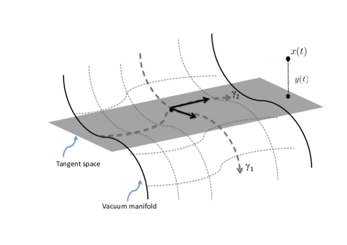
Figure 1: Pictorical representation of the projection of the path $x(t)$ to onto the vacuum field manifold. A path $x(t)$ is represented by a point in this picture. The constraints (5) imply that the the fluctuation field $y(t)$ is perpendicular to the plane tangent to the manifold in the point of the curvilinear abscissas $\gamma=\bar{\gamma}$.

The path integral (13) can be formally re-written as

$$Z(T;x_{i},x_{f})=\int\prod_{l=1}^{k}\leavevmode\nobreak\ d\leavevmode\nobreak\ \gamma_{l}\leavevmode\nobreak\ e^{-\frac{1}{\hbar}F(\gamma_{1},\ldots,\gamma_{k})},$$ (14)

where $F(\gamma)$ is defined as

$$F(\gamma)=-\hbar\log\int_{y(-T/2)=0}^{y(T/2)=0}\mathcal{D}y\leavevmode\nobreak\ \leavevmode\nobreak\ \left(\prod_{i}\delta^{(k)}(y(t)\cdot g_{\gamma_{i}}(t,\bar{\gamma}))\right)\leavevmode\nobreak\ \Phi[\tilde{x}(t;\gamma)+y(t)]e^{-\frac{1}{\hbar}S[\tilde{x}(t;\gamma)+y(t)]}.$$ (15)

Some comments on what we have done so far are in order. First of all we stress that $Z(T;x_{i},x_{f})$ can be interpreted as the partition function of a system with a finite number of degrees of freedom $\gamma_{1},\ldots,\gamma_{k}$. The term $F(\gamma_{1},\ldots,\gamma_{k})$ is the analog of the (free) energy in statistical physics an will be referred to as the effective interaction.

Let us now address the problem of how to compute $F(\gamma_{1},\ldots,\gamma_{k})$, using lattice simulations. Let $\{x_{1}(t),\ldots,x_{N_{conf}}(t)\}$ be a statistically representative ensemble of $N_{conf}$ paths (i.e. obtained by means of lattice simulations). The coordinates $(\Phi_{1},\ldots,\Phi_{k})$ of each of such paths are specified by the Eq.s (II)-(10). Using the definition (4) and the orthogonality conditions (5) we obtain a set of $k$ non-linear Eq.s for the $\gamma_{1},\ldots,\gamma_{k}$ variables:

$$\Phi_{1}[x(t)]=(x(t)\cdot g_{\gamma_{1}}(t,\bar{\gamma})) = (\tilde{x}(t;\gamma)\cdot g_{\gamma_{1}}(t,\bar{\gamma}))\equiv\Psi_{1}(\gamma)$$

$$...$$

$$\Phi_{k}[x(t)]=(x(t)\cdot g_{\gamma_{k}}(t,\bar{\gamma})) = (\tilde{x}(t;\gamma)\cdot g_{\gamma_{k}}(t,\bar{\gamma}))\equiv\Psi_{k}(\gamma).$$ (17)

Note that, while the coordinates $\Phi_{1},\ldots,\Phi_{k}$ on the left-hand-side depend on the path $x(t)$, the functions $\Psi_{1}(\gamma),\ldots,\Psi_{k}(\gamma)$ on the right-hand-side depend only on the set of collective coordinates $(\gamma_{1},\ldots,\gamma_{k})$ and are determined by the choice of the background field manifold and of the parameter $\bar{\gamma}$. Hence, by solving numerically such a system of Eq.s, a value for the curvilinear coordinates can be assigned to each configuration. Repeating this procedure for the entire ensemble of lattice configurations $x_{1}(t),\ldots,x_{N_{conf}}(t)$ one determines the probability density $\mathcal{P}(\gamma_{1},\ldots,\gamma_{k})$, which relates directly to the effective interaction

$$F(\gamma_{1},\ldots,\gamma_{k})=-\frac{1}{\hbar}\leavevmode\nobreak\ \log\mathcal{P}(\gamma_{1},\ldots,\gamma_{k}).$$ (18)

The effective theory defined by the partition function (14) allows to perform approximate calculations of the vacuum expectation value of arbitrary operators $\hat{O}(t)$,

$$\langle\hat{O}(t)\rangle=\frac{\int\mathcal{D}x\leavevmode\nobreak\ O[x(t)]\leavevmode\nobreak\ e^{-\frac{1}{\hbar}S[x]}}{\int\mathcal{D}xe^{-\frac{1}{\hbar}S[x]}}.$$ (19)

In fact, if the vacuum manifold contains the physically important vacuum configurations, then $O[x(t)]\simeq O[\tilde{x}(t;\gamma)]$ and

$$\langle\hat{O}(t)\rangle\simeq\frac{\int\prod_{l=1}^{k}\leavevmode\nobreak\ d\leavevmode\nobreak\ \gamma_{l}\leavevmode\nobreak\ O[\tilde{x}(\gamma_{1},\ldots,\gamma_{k})]\leavevmode\nobreak\ e^{-\frac{1}{\hbar}F(\gamma_{1},\ldots,\gamma_{k})}}{\int\prod_{l=1}^{k}\leavevmode\nobreak\ d\leavevmode\nobreak\ \gamma_{l}\leavevmode\nobreak\ e^{-\frac{1}{\hbar}F(\gamma_{1},\ldots,\gamma_{k})}}.$$ (20)

We note that, while the partition function (14) is independent on the choice of $\bar{\gamma}$ — which specifies the system of coordinates on the manifold— the effective interaction $F(\gamma)$ and vacuum expectation values of operators may in principle depend on such a parameter. However, such a dependence is generated only by the projection of paths which contain very large fluctuations, i.e. lie far from the vacuum manifold. To see this, let us consider the projection of a configuration $x(t)$ which lies very close to a point on the vacuum manifold $\tilde{x}(t;\gamma^{\prime})$, i.e.

$$||x(t)-\tilde{x}(t;\gamma^{\prime})||\simeq 0,$$ (21)

for some $\gamma^{\prime}$. Then, the projection Eq.s (II)-(17) read:

$$(x(t)\cdot g_{\gamma_{1}}(t,\bar{\gamma}))\simeq(\tilde{x}(t;\gamma^{\prime})\cdot g_{\gamma_{1}}(t,\bar{\gamma})) = (\tilde{x}(t;\gamma)\cdot g_{\gamma_{1}}(t,\bar{\gamma}))$$

$$...$$

$$(x(t)\cdot g_{\gamma_{k}}(t,\bar{\gamma}))\simeq(\tilde{x}(t;\gamma^{\prime})\cdot g_{\gamma_{k}}(t,\bar{\gamma})) = (\tilde{x}(t;\gamma)\cdot g_{\gamma_{k}}(t,\bar{\gamma})).$$ (23)

A solution of such set of Eq.s is trivially $\gamma^{\prime}=\gamma$, for any choice of the projection point $\bar{\gamma}$. If the vacuum field manifold captures the physically important configurations, the vacuum expectation values of operators $\hat{O}(t)$ will be dominated by the configurations in the functional vicinity of the manifold. In the limit in which the relevant configurations are only those very close to the manifold, the system of Eq.s (II)-(17) have a unique solution and the expressions (19) become independent on the choice of the coordinate system on the manifold, i.e. of the parameter $\bar{\gamma}$. Clearly, this condition can be verified by comparing the results obtained projecting onto different points of the manifold.

In the rest of this paper, we shall illustrate how this method is implemented in practice, in the specific case of the one-dimensional quantum double-well problem.

III Application to the quantum mechanical double well problem

The discussion made so far has been completely general: Eq.s (14) and (15) hold for an arbitrary choice of the potential $U(x)$, of the vacuum field manifold $\mathcal{M}$ and of the boundary conditions $x_{i}$ and $x_{f}$. As an illustrative example, let us now restrict our attention to the specific system defined by the potential

$$U(x)=m\alpha\left(x^{2}-\beta^{2}\right)^{2},$$ (24)

where $m$ is the mass of the particle. We consider the path integral with periodic boundary conditions (see Eq.  1)

$$x_{i}=x_{f}=-\beta\leavevmode\nobreak\ \qquad\textrm{( or equivalently:}\leavevmode\nobreak\ x_{i}=x_{f}=+\beta\leavevmode\nobreak\ ).$$ (25)

In this specific system, a choice of the effective degrees of freedom is suggested semi-classical arguments. We choose the vacuum field manifold to be the one generated by the superposition of $N$ instantons and $N$ antiinstantons. Obviously, the choice of the optimal number of pseudo-particles depends on the time interval $T$. If the barrier is sufficiently high, one can fix $N$ from the semi-classical tunneling rate colman

$$2N\simeq\kappa T,$$ (26)

where $\kappa$ is the one-instanton measure

$$\kappa\simeq 4\sqrt{\frac{2(2\alpha)^{3/2}\beta^{2}}{\pi\hbar}}.$$ (27)

The curvilinear coordinates $\gamma_{1}=t_{1},\gamma_{2}=\bar{t}_{1},\ldots,\gamma_{2N-1}=t_{N},\gamma_{2N}=\bar{t}_{N}$ represent the collective coordinates of each instanton or antiinstanton, i.e. their positions in the imaginary time axis. In particular, we adopt the so-called "sum-ansatz", which consists in simply adding-up the instanton and antiinstanton fields:

$$\tilde{x}_{S_{2N}}(t;t_{1},\ldots\bar{t}_{N})\equiv-\beta+\sum_{k=1}^{N}\left[\hat{x}_{I}(t-t_{k})+\hat{x}_{\bar{I}}(t-\bar{t}_{k})\right],$$ (28)

where we have labeled with $t_{1},\ldots t_{N}$ ($\bar{t}_{1},\ldots,\bar{t}_{N}$) the centers of the instantons (antiinstantons). The path integral, re-written as in Eq.(14) reads

$$Z[T;-\beta,-\beta]=\int dt_{1},\int d\bar{t}_{1}\ldots\int dt_{N}\int d\bar{t}_{N}\leavevmode\nobreak\ e^{-\frac{1}{\hbar}\leavevmode\nobreak\ F(t_{1},\bar{t}_{1},\ldots,t_{N},\bar{t}_{N})}$$ (29)

We note that there are only two choices of such collective coordinates for which the field configuration (28) becomes an exact solution of the Euclidean EoM:

1. When all nearest neighbour instanton-antiinstantons pairs are infinitely separated from each other, i.e.

   $$|t_{i}-\bar{t}_{i}|\to\infty,|t_{i+1}-\bar{t}_{i}|\to\infty$$

2. When all nearest neighbour instanton-antiinstantons pairs are infinitely close to each other, i.e.

   $$t_{i}=\bar{t}_{i}$$

   .

In the former case, one obtains a dilute instanton gas configuration. In the latter case, all pairs annihilate and the field reduces a trivial classical vacuum, i.e. $x(t)=-\beta$. For any other choice of the collective coordinates $t_{1},\ldots,\bar{t}_{N}$, the field configuration (28) is not an extremum of the action.

The relative statistical weight of each configuration in the path integral (2) is provided by the exponential factor appearing in Eq. (29), which plays the role of the free energy in the statistical mechanical analogy. Hence, the function $F(t_{1},\ldots,\bar{t}_{N})$ expresses the statistical and dynamical correlations between the pseudo-particles, induced by all other field configurations in the path integral. For example, in the high barrier limit in which the semi-classical dilute instanton gas approximation is justified, one has

$$e^{-\frac{1}{\hbar}\leavevmode\nobreak\ F(t_{1},\ldots,\bar{t}_{N})}\simeq\theta(\bar{t}_{1}-t_{1})\leavevmode\nobreak\ \theta(t_{2}-\bar{t}_{1})\ldots\theta(\bar{t}_{N}-t_{N})\leavevmode\nobreak\ \kappa^{2N}.$$ (30)

As the height of the barrier is adiabatically reduced, the dilute instanton gas approximation becomes worse and worse and eventually breaks down. In this regime, the vacuum fields behave as an interacting liquid and the effective interaction $F(t_{1},\ldots,\bar{t}_{N})$ deviates from the expression (30) and can be written as

$$F(\bar{t}_{1},\ldots,\bar{t}_{N})\simeq\sum_{i=1}^{N}F^{IA}_{2}(\bar{t}_{i}-t_{i})+F^{AI}_{2}(t_{i+1}-\bar{t}_{i}),$$ (31)

where $F^{IA}_{2}$ ($F^{AI}_{2}$) expresses the two-body instanton-antiinstanton (antiinstanton- instanton) correlations . For very low barriers, the average instanton distance becomes smaller than the instanton size, and the pseudoparticles "melt". Clearly, in such a regime, instantons and antiinstanton fields no longer represent a good choice of low-energy vacuum degrees of freedom. In the remaining of this work, we shall consider systems for which the dilute liquid regime is appropriate.

In order to compute $F^{IA}_{2}(t^{\prime}-t)$ and $F^{AI}_{2}(t^{\prime}-t)$ it is convenient to integrate out from (29) all instanton degrees of freedom, except those of a single pair of pseudo particles. To this end, we rewrite the path integral as :

$$Z[T;-\beta,-\beta] = \frac{1}{2}\left[\int dt_{1}\!\int d\bar{t}_{1}\left(\int dt_{2}\leavevmode\nobreak\ d\bar{t}_{2}\ldots d\bar{t}_{N}\leavevmode\nobreak\ e^{-\frac{1}{\hbar}F}\right)+\int d\bar{t}_{1}\int dt_{2}\leavevmode\nobreak\ \left(\int dt_{1}\,d\bar{t}_{2}\,dt_{3}\ldots d\bar{t}_{N}\leavevmode\nobreak\ e^{-\frac{1}{\hbar}F}\right)\right]$$ (32)

$$= \frac{1}{2}\leavevmode\nobreak\ \left(\int dt^{\prime}\int dt\leavevmode\nobreak\ g_{2}^{IA}(t^{\prime}-t)+\int dt\int dt^{\prime}\leavevmode\nobreak\ g_{2}^{AI}(t^{\prime}-t)\right).$$ (33)

The first term corresponds to the case in which the pseudo-particle of coordinate $t$ is an instanton, while the second of coordinate $t^{\prime}$ is an anti-instanton and $g_{2}^{IA}(t^{\prime}-t)$ is the corresponding pair-correlation function. Conversely, the second term corresponds to the case in which the pseudo-particle at $t$ is an anti-instanton and that at $t^{\prime}$ is an instanton. In the dilute liquid regime, the functions $g^{IA(AI)}(t^{\prime}-t)$ relate directly to $F^{IA(AI)}_{2}(t^{\prime}-t)$ by

$$e^{-\frac{1}{\hbar}\leavevmode\nobreak\ F^{IA(AI)}_{2}(t^{\prime}-t)}\propto\leavevmode\nobreak\ g_{2}^{IA(AI)}(t^{\prime}-t),$$ (34)

where the proportionality factor is controlled by the density.

In order to extract the instanton-antiinstanton pair correlation function $g^{IA}_{2}$ we consider the path integral with boundary condition $x_{f}=x_{i}=-\beta$ and parametrize a generic configuration $x(t)$ using the sum ansatz for an instanton-antiiinstanton pair, Eq.(28)

$$x(t) = \tilde{x}^{IA}_{S_{2}}\left(t;t_{1},t_{2}\right)+y(t)$$ (35)

$$= -\beta\left\{1-\tanh\!\left[\sqrt{2\alpha}\,\beta\,(t-t_{1})\right]+\tanh\!\left[\sqrt{2\alpha}\,\beta\,(t-t_{2})\right]\right\}+y(t)$$ (36)

where $y(t)$ is a configuration of boundary conditions $y(\pm T/2)=0$, and $t_{1}$ and $t_{2}$ are the coordinates of the two pseudoparticles, in the Euclidean time axis. Conversely, in order to evaluate $g_{2}^{AI}$, one should consider the path integral with boundary conditions $x_{f}=x_{i}=\beta$ and adopt a vacuum manifold based on the anti-instanton instanton pair:

$$x(t) = \tilde{x}^{AI}_{S_{2}}\left(t;t_{1},t_{2}\right)+y(t)$$ (37)

$$= \beta\left\{1-\tanh\!\left[\sqrt{2\alpha}\,\beta\,(t-t_{1})\right]+\tanh\!\left[\sqrt{2\alpha}\,\beta\,(t-t_{2})\right]\right\}+y(t).$$ (38)

Since the two calculations are identical, in the following we shall focus on determining $g_{2}^{IA}$ and the $IA$ suffix will be implicitly assumed.

It is convenient to introduce the relative variables

$$\chi = \frac{1}{2}\leavevmode\nobreak\ (t_{1}+t_{2}),$$

$$\xi = t_{2}-t_{1}.$$

Notice that variable $\chi$ is the "center of mass" of the pair, while $\xi$ represents the "relative distance" between the instanton and antiinstanton. Notice also that Eq.(33) implies

$$F_{2}(t_{1},t_{2})=F_{2}(t_{2}-t_{1})\equiv F_{2}(\xi),$$ (39)

that is to say we expect the effective interaction to be independent from the center of mass of the pair. This is a consequence of the time translational invariance of the vacuum.

We recall that the multi-instanton field configuration and the fluctuation field have to fulfill the orthogonality conditions (5), which is enforced in a specific point $\gamma=\bar{\gamma}$ of the manifold. The basis vector of the tangent space of the manifold defined by the sum ansatz (28) are, for an arbitrary point $\gamma=(\bar{t}_{1},\bar{t}_{2})$

$$g_{t_{1}}(t;\bar{t}_{1},\bar{t}_{2}) = \left.\phantom{\int}\partial_{t_{1}}\tilde{x}_{S_{2}}(t;t_{1},t_{2})\leavevmode\nobreak\ \right|_{{t_{1}=\bar{t}_{1},t_{2}=\bar{t}_{2}}}=-\sqrt{2\alpha}\beta^{2}\textrm{sech}^{2}\left[\sqrt{2\alpha}\beta(t-\bar{t}_{1})\leavevmode\nobreak\ \right]$$ (40)

$$g_{t_{2}}(t;\bar{t}_{1},\bar{t}_{2}) = \left.\phantom{\int}\partial_{t_{2}}\tilde{x}_{S_{2}}(t;t_{1},t_{2})\leavevmode\nobreak\ \right|_{{t_{1}=\bar{t}_{1},t_{2}=\bar{t}_{2}}}=\sqrt{2\alpha}\beta^{2}\textrm{sech}^{2}\left[\sqrt{2\alpha}\beta(t-\bar{t}_{2})\leavevmode\nobreak\ \right]$$ (41)

Equivalently, in terms of the $\chi$ and $\xi$ coordinates, the basis vectors of the tangent space in the generic point $\gamma=(\xi,\chi)$ read

$$g_{\chi}(t;\bar{\chi},\bar{\xi}) = \left.\phantom{\int}\partial_{\chi}\leavevmode\nobreak\ \tilde{x}_{S_{2}}\left(t;\chi-\frac{1}{2}\xi,\chi+\frac{1}{2}\xi\right)\leavevmode\nobreak\ \right|_{{\chi=\bar{\chi},\xi=\bar{\xi}}}$$ (42)

$$= \sqrt{2\alpha}\beta^{2}\left\{\textrm{sech}^{2}\left[\sqrt{2\alpha}\beta\left(t-\bar{\chi}-\frac{\bar{\xi}}{2}\right)\right]-\textrm{sech}^{2}\left[\sqrt{2\alpha}\beta\left(t-\bar{\chi}+\frac{\bar{\xi}}{2}\right)\right]\right\}$$

$$g_{\xi}(t;\bar{\chi},\bar{\xi}) = \left.\phantom{\int}\partial_{\xi}\leavevmode\nobreak\ \tilde{x}_{S_{2}}\left(t;\chi-\frac{1}{2}\xi,\chi+\frac{1}{2}\xi\right)\leavevmode\nobreak\ \right|_{{\chi=\bar{\chi},\xi=\bar{\xi}}}$$ (43)

$$= \sqrt{\frac{\alpha}{2}}\beta^{2}\left\{\textrm{sech}^{2}\left[\sqrt{2\alpha}\beta\left(t-\bar{\chi}-\frac{\bar{\xi}}{2}\right)\right]+\textrm{sech}^{2}\left[\sqrt{2\alpha}\beta\left(t-\bar{\chi}+\frac{\bar{\xi}}{2}\right)\right]\right\},$$

Hence, without loss of generality, in the following we shall consider

$$x(t;\chi,\xi) = -\beta\left\{1-\tanh\!\left[\sqrt{2\alpha}\,\beta\,\left(t-\chi+\frac{\xi}{2}\right)\right]+\tanh\!\left[\sqrt{2\alpha}\,\beta\,\left(t-\chi-\frac{\xi}{2}\right)\right]\right\}+y(t)$$ (44)

with the conditions

$$\bigg{(}y(t)\cdot g_{\chi}(t;\bar{\chi},\bar{\xi})\bigg{)}=0,$$ (45)

$$\bigg{(}y(t)\cdot g_{\xi}(t;\bar{\chi},\bar{\xi})\bigg{)}=0.$$ (46)

Although our ultimate goal is to evaluate $F_{2}^{IA}(\xi)$ and $F_{2}^{IA}(\xi)$ in a fully non-perturbative way, it is instructive to discuss first a perturbative analysis, which yields information about the contribution to the quantum effective interactions in the short instanton-antiinstanton distance limit. Such a calculation isl be presented in the next section, while the fully non-perturbative calculation is reported in section V.

IV Perturbative Calculation

Perturbation theory deals with small quantum fluctuations around a classical vacuum. In particular, a calculation of $F_{2}^{IA}(\xi)$ and $F_{2}^{IA}(\xi)$ at small $\xi$ requires to assign to each point in the vicinity of the trivial vacuum

$$\tilde{x}_{S_{2}}\equiv-\beta$$ (47)

a point on the intanton-antiinstanton functional manifold. Since quantum fluctuations can be arbitrarily small, the orthogonality conditions (45) and (46) have to be imposed at a point which is arbitrarily close to the same classical vacuum. In principle, the most natural choice would be impose the orthogonality conditions at the classical vacuum. However, problems arise due to the fact that it is not possible to define the tangent space in such a point, since

$$g_{\chi}(t;\bar{\chi},0)\equiv 0,$$ (48)

for all $\bar{\chi}$. To overcome this difficulty, in the following we use the stochastic quantization formalism to construct a rigorous approach in which the tangent space which is defined at a point which is arbitrarily close to classical point, but does not coincide with it.

Let us begin by briefly reviewing Pairsi and Wu quantization technique parisi . The starting point is to allow the field configuration $x(t)$ to depend on an additional parameter, the so-called stochastic ”time” $\tau$. The dynamics of the field in such an additional dimension is postulated to obey a Langevin equation:

$$x^{\prime}(t,\tau)\equiv\frac{d}{d\tau}\leavevmode\nobreak\ x(t,\tau)=-k\frac{\delta\,S[x]}{\delta\,x(t,\tau)}+\sqrt{\hbar}\,\eta(t,\tau),$$ (49)

where $k$ is an arbitrary diffusion coefficient and $\eta(t,\tau)$ Gaussian distributed stochastic field

$$P[\eta] \propto \exp\left\{-\frac{1}{4k}\int_{-\infty}^{\infty}\mbox{d}t\int_{0}^{\infty}\mbox{d}\tau\,\,\eta^{2}(t,\tau)\right\}$$ (50)

which obeys the fluctuation-dissipation relationship

$$\langle\eta(t,\tau)\eta(t^{\prime},\tau^{\prime})\rangle = \int\mathcal{D}\eta\,\eta(t,\tau)\eta(t^{\prime},\tau^{\prime})P[\eta]=2\leavevmode\nobreak\ k\leavevmode\nobreak\ \delta(t^{\prime}-t)\leavevmode\nobreak\ \delta(\tau^{\prime}-\tau).$$ (51)

For any value of the stochastic time $\tau$, the probability to for the field to assume a given configuration $x(t,\tau)$ is described by a (functional) probability distribution $\mathcal{P}[x](\tau)$, which is a solution of the Fokker-Planck Eq. associated to the Langevin Eq. (49):

$$\frac{d}{d\tau}\mathcal{P}[x]=k\leavevmode\nobreak\ \frac{\delta^{2}}{\delta x^{2}}P[x]+k\leavevmode\nobreak\ \frac{\delta}{\delta x}\left(\mathcal{P}[x]\leavevmode\nobreak\ \frac{\delta S[x]}{\delta x}\right)$$ (52)

A general property of the Fokker Planck Eq. is that its solutions converge to the static, "Boltzmann" weight, in the long time limit:

$$\mathcal{P}[x]\stackrel{{\scriptstyle(\tau\to\infty)}}{{\rightarrow}}\frac{1}{\int\mathcal{D}x(t)\exp\Big{\{}-\frac{1}{\hbar}S[x(t)]\Big{\}}}\exp\Big{\{}-\frac{1}{\hbar}S[x(t)]\Big{\}},$$ (53)

regardless of the initial condition, $x(t,\tau=0)$ and of the value of the diffusion coefficient $k$. Hence, the Langevin Eq. (49) generates configurations which, at equilibrium, are distributed according to the statistical weight appearing in the Euclidean quantum path integral. Such configurations can be used to compute quantum mechanical Green’s functions.

In stochastic perturbation theory, a generic path $x(t,\tau)$ obeying Langevin Eq. (49) with boundary conditions (1) is written as a power series in $\varepsilon=\sqrt{\hbar}$:

$$x(t,\tau) = \sum_{i=i}^{\infty}\varepsilon^{i}x_{i}(t,\tau),$$ (54)

$x_{0}(t,\tau)$ is the classical content of the path, while all other terms represent quantum corrections. In the double-well problem, the classical solution with boundary conditions (25) is $x_{0}(t,\tau)=-\beta$.

By inserting the expansion (54) into the Langevin Eq. (49) and matching the Left-Hand-Side (LHS) and Right-Hand-Side (RHS), order by order in $\varepsilon$, one generates a tower of coupled stochastic differential Eq.s, for the components $x_{i}(t,\tau)$, which appear in Eq. (54):

$$O(\varepsilon^{0}): x^{\prime}_{0}(t,\tau)=k\,m\left(\partial_{t}^{2}-4\alpha\leavevmode\nobreak\ [x_{0}^{2}(t,\tau)-\beta^{2}]\leavevmode\nobreak\ \right)\leavevmode\nobreak\ x_{0}(t,\tau)$$ (55)

$$O(\varepsilon^{1}): x_{1}^{{}^{\prime}}(t,\tau)=k\,m\left(\partial_{t}^{2}-4\alpha\leavevmode\nobreak\ [3\,x_{0}^{2}(t,\tau)-\beta^{2}]\leavevmode\nobreak\ \right)\leavevmode\nobreak\ x_{1}(t,\tau)+\eta(t,\tau)$$ (56)

$$O(\varepsilon^{2}): x_{2}^{{}^{\prime}}(t,\tau)=k\,m\left[\left(\partial_{t}^{2}-4\alpha\leavevmode\nobreak\ [3\,x_{0}^{2}(t,\tau)-\beta^{2}]\leavevmode\nobreak\ \right)\leavevmode\nobreak\ x_{2}(t,\tau)-12\alpha\,x_{0}(t,\tau)x_{1}^{2}(t,\tau)\right]$$ (57)

$$O(\varepsilon^{3}): x_{3}^{{}^{\prime}}(t,\tau)=k\,m\left[\left(\partial_{t}^{2}-4\alpha\leavevmode\nobreak\ [3\,x_{0}^{2}(t,\tau)-\beta^{2}]\leavevmode\nobreak\ \right)\leavevmode\nobreak\ x_{3}(t,\tau)-4\alpha\,x_{1}^{3}(t,\tau)-24\alpha x_{0}(t,\tau)x_{1}(t,\tau)x_{2}(t,\tau)\right]$$

$$\ldots$$

In practice, the perturbative expansion is truncated and one solves a finite set of stochastic differential Eq.s, starting from a given initial condition. For example, truncating the expansion to order $\varepsilon^{2}$ and choosing the initial condition

$$x_{0}(t,\tau=0) = -\beta,$$ (59)

$$x_{i}(t,\tau=0) = 0,\qquad(i=1,2,\ldots),$$ (60)

which corresponds to the classical vacuum state, we find

$$x_{0}(t,\tau) = -\beta$$ (61)

$$x_{1}(t,\tau) = \int_{-\infty}^{\infty}\frac{\mbox{d}\omega}{2\pi}e^{-i\omega t}\int_{0}^{\infty}\mbox{d}\tau^{{}^{\prime}}\theta\left[\tau-\tau^{{}^{\prime}}\right]e^{-km(8\alpha\beta^{2}+\omega^{2})(\tau-\tau^{{}^{\prime}})}\tilde{\eta}(\omega,\tau^{{}^{\prime}})$$ (62)

$$x_{2}(t,\tau) = 12\alpha\beta km\int_{-\infty}^{\infty}\frac{\mbox{d}\omega}{2\pi}e^{-i\omega t}\int_{0}^{\infty}\mbox{d}\tau^{{}^{\prime}}\theta\left[\tau-\tau^{{}^{\prime}}\right]e^{-km(8\alpha\beta^{2}+\omega^{2})(\tau-\tau^{{}^{\prime}})}\leavevmode\nobreak\ \int_{-\infty}^{\infty}\mbox{d}t^{{}^{\prime}}e^{i\omega t^{{}^{\prime}}}x^{2}_{1}(t^{{}^{\prime}},\tau^{{}^{\prime}}).$$ (63)

The corresponding perturbative solution is

$$x(t,\tau)=x_{0}(t,\tau)+\varepsilon x_{1}(t,\tau)+\varepsilon^{2}x_{2}(t,\tau).$$ (64)

It is important to stress that only the asymptotic equilibrium solution $x(t,\tau=\infty)$ enters in the evaluation of physical observables. Such equilibrium solutions are independent on the choice of the initial condition of the perturbative stochastic equations (55)-(IV).

Let us now show how the stochastic perturbation theory technique can be used to gain information about the $F^{IA}_{2}(\xi)$ and $F^{AI}_{2}(\xi)$ distributions. To this end, we begin by decomposing the field as in Eq. (4),

$$x(t)\equiv\tilde{x}_{S_{2}}(t;t_{1},t_{2})+y(t).$$ (65)

Next we need to promote the manifold field $\tilde{x}(t;\chi,\xi)$ and fluctuation field $y(t)$ to dynamical variables, under the stochastic time evolution. There is some freedom associated to the definition of such a stochastic dynamics. For example, a possible choice may be one in which the $\tau$ dependence enters entirely through the fluctuation field $y(t,\tau)$, while the smooth vacuum field $\tilde{x}_{S_{2}}$ is assumed to be static, under stochastic evolution, i.e. $\tilde{x}_{S_{2}}(t,\tau)=\tilde{x}_{S_{2}}(t)$. Instead, a crucial point of the present approach is to make a different choice and allow both the fluctuation field and the smooth vacuum field to vary with the stochastic time $\tau$. This is done in practice by promoting the curvilinear coordinates $\xi$ and $\chi$ to dynamical stochastic degrees of freedom granati , i.e. $\xi\rightarrow\xi(\tau)$ and $\chi\rightarrow\chi(\tau)$. Consequently, at a generic stochastic instant $\tau$, the quantum field $x(t,\tau)$ reads:

$$x(t,\tau) = \tilde{x}_{S_{2}}\left(t;\chi(\tau)-\frac{1}{2}\xi(\tau),\chi(\tau)+\frac{1}{2}\xi(\tau)\right)+y(t,\tau).$$ (66)

Let us now construct a perturbative solution of the Langevin Eq. (49), based on the decomposition (66). We recall that the multi-instanton field is not a classical solution of the EoM, except in the points where $\xi=0$. As a consequence, quantum corrections will appear not only in the fluctuation field, but also in the background field. To account for this fact, we expand $y(t,\tau)$, $\chi(\tau)$ and $\xi(\tau)$ as power series in $\varepsilon=\sqrt{\hbar}$:

$$y(t,\tau) = \sum_{i=1}^{\infty}\varepsilon^{i}y_{i}(t,\tau)$$ (67)

$$\chi(\tau) = \sum_{i=0}^{\infty}\varepsilon^{i}\leavevmode\nobreak\ \chi_{i}(\tau)$$ (68)

$$\xi(\tau) = \sum_{i=0}^{\infty}\varepsilon^{i}\leavevmode\nobreak\ \xi_{i}(\tau)$$ (69)

Let us now define the tangent space in a generic point $\bar{\xi},\bar{\chi}$ of the manifold. It is possible to show that the orthogonality conditions (45) and (46) hold order-by-order in perturbation theory and at any stochastic time i.e.:

$$\bigg{(}y_{i}(t,\tau)\cdot g_{\chi}(t;\bar{\chi},\bar{\xi})\bigg{)}=0;$$ (70)

$$\bigg{(}y_{i}(t,\tau)\cdot g_{\xi}(t;\bar{\chi},\bar{\xi})\bigg{)}=0,\qquad\forall i,\forall\tau.$$ (71)

From Eq.s (54), (67), (68) and (69) it is immediate to obtain an expression for each of the $x_{i}(t,\tau)$ components in Eq. (54):

$$x_{i}(t,\tau)\equiv\leavevmode\nobreak\ \left.\frac{1}{i!}\frac{\partial^{i}}{\partial\varepsilon^{i}}\leavevmode\nobreak\ \left(\hat{x}_{S_{2}}\left(t;\sum_{n=0}^{\infty}\varepsilon^{n}\chi_{n},\sum_{m=0}^{\infty}\varepsilon^{m}\xi_{m}\right)+\sum_{l=1}^{\infty}\varepsilon^{l}y_{l}(t,\tau)\leavevmode\nobreak\ \right)\leavevmode\nobreak\ \right|_{\varepsilon=0}$$ (72)

For example, the first orders are

$$x_{0}(t,\tau) = \tilde{x}_{S_{2}}\left(t;\chi_{0}-\frac{\xi_{0}(\tau)}{2},\chi_{0}+\frac{\xi_{0}(\tau)}{2}\right)$$ (73)

$$x_{1}(t,\tau) = \chi_{1}(\tau)\leavevmode\nobreak\ g_{\chi}\big{(}t;\chi_{0},\xi_{0}(\tau)\big{)}+\xi_{1}(\tau)\leavevmode\nobreak\ g_{\xi}\big{(}t;\chi_{0},\xi_{0}(\tau)\big{)}+y_{1}(t,\tau)\phantom{\bigg{\{}}$$ (74)

$$x_{2}(t,\tau) = \chi_{2}(\tau)\leavevmode\nobreak\ g_{\chi}\big{(}t;\chi_{0},\xi_{0}(\tau)\big{)}+\xi_{2}(\tau)\leavevmode\nobreak\ g_{\xi}\big{(}t;\chi_{0},\xi_{0}(\tau)\big{)}+\phantom{\bigg{\{}}$$

$$-\frac{1}{2}\left(\chi_{1}^{2}(\tau)+\frac{\xi^{2}_{1}(\tau)}{4}\right)\leavevmode\nobreak\ \dot{g}_{\chi}\big{(}t,\chi_{0},\xi_{0}(\tau)\big{)}-\chi_{1}(\tau)\leavevmode\nobreak\ \xi_{1}(\tau)\leavevmode\nobreak\ \dot{g}_{\xi}\big{(}t,\chi_{0},\xi_{0}(\tau)\big{)}+y_{2}(t,\tau)\phantom{\bigg{\{}}$$

$$\ldots .,$$

where we have used the fact that $\chi_{0}$ is independent on $\tau$. The terms on the LHS of Eq.s (73)-(IV) coincide with the perturbative solution results (61)-(63). On the other hand, the terms on the RHS represent the decomposition of the same functions in terms of the low-energy vacuum field configurations and of the corresponding fluctuation fields.

In order to make contact with the effective interaction, we need to introduce the tangent space which enters the projection Eq.s (70) and (71). At this point, we need face the above mentioned problem that the tangent space at the classical vacuum $-\beta$ is not defined. To overcome this problem, we let the tangent space vary with the stochastic time in such a way that the point $\bar{\xi},\bar{\chi}$ asymptotically approaches the classical vacuum, but does not coincide with it at any finite $\tau$. In practice, we promote $\bar{\xi}$ to a stochastic variable and we impose

$$\bar{\xi}(\tau)\stackrel{{\scriptstyle\tau\rightarrow\infty}}{{\rightarrow}}0.$$ (76)

In particular, we choose $\bar{\xi}(\tau)\equiv\xi_{0}(\tau)$, since $\xi_{0}(\tau\to\infty)\to 0$.

Using such a decomposition, we are now in a condition to analytically compute arbitrary moments of the equilibrium distribution for $\chi$ and $\xi$, i.e. $\langle\xi^{k}\rangle$ and $\langle\chi^{k}\rangle$. By projecting and inverting Eq.s (74) and (IV), we obtain the following expression for the collectives coordinates up to $\mathcal{O}(\hbar)$

$$\chi_{1}(\tau) = \frac{\left(x_{1}(t,\tau)\cdot g_{\chi}(t;\chi_{0},\xi_{0}(\tau))\right)}{\left(g_{\chi}(t;\chi_{0},\xi_{0}(\tau)\cdot g_{\chi}(t;\chi_{0},\xi_{0}(\tau)\right)},$$ (77)

$$\xi_{1}(\tau) = \frac{\left(x_{1}(t,\tau)\cdot g_{\xi}(t;\chi_{0},\xi_{0}(\tau))\right)}{\left(g_{\xi}(t;\chi_{0},\xi_{0}(\tau)\cdot g_{\xi}(t;\chi_{0},\xi_{0}(\tau)\right)},$$ (78)

$$\chi_{2}(\tau) = \frac{\left(x_{2}(t,\tau)\cdot g_{\chi}(t;\chi_{0},\xi_{0}(\tau))\right)+\chi_{1}(\tau)\xi_{1}(\tau)\left(\dot{g}_{\xi}(t;\chi_{0},\xi_{0}(\tau))\cdot g_{\chi}(t;\chi_{0},\xi_{0}(\tau))\right)}{\left(g_{\chi}(t;\chi_{0},\xi_{0}(\tau))\cdot g_{\chi}(t;\chi_{0},\xi_{0}(\tau))\right)},$$ (79)

$$\xi_{2}(\tau) = \frac{\left(x_{2}(t,\tau)\cdot g_{\xi}(t;\chi_{0},\xi_{0}(\tau))\right)+\frac{1}{2}\left(\chi_{1}^{2}(\tau)+\frac{1}{2}\xi^{2}_{1}(\tau)\right)\left(\dot{g}_{\chi}(t;\chi_{0},\xi_{0}(\tau))\cdot g_{\xi}(t;\chi_{0},\xi_{0}(\tau))\right)}{\left(g_{\xi}(t;\chi_{0},\xi_{0}(\tau)\cdot g_{\xi}(t;\chi_{0},\xi_{0}(\tau)\right)},$$ (80)

$$\ldots$$ . (81)

Using the fluctuation-dissipation relationships (51), and the fact that $\xi_{0}(\tau)$ is independent from $\eta(t,\tau)$ we find

$$\langle\chi_{1}(\tau)\rangle = 0$$ (82)

$$\langle\chi_{2}(\tau)\rangle = 0$$ (83)

$$\langle\xi_{1}(\tau)\rangle = 0$$ (84)

$$\langle\xi_{2}(\tau)\rangle = \frac{\langle x_{2}(t,\tau)\rangle\left(1\cdot g_{\xi}(t;\chi_{0},\xi_{0}(\tau))\right)+\frac{1}{2}\left(\langle\chi_{1}^{2}(\tau)\rangle+\frac{1}{2}\langle\xi^{2}_{1}(\tau)\rangle\right)\left(\dot{g}_{\chi}(t;\chi_{0},\xi_{0}(\tau))\cdot g_{\xi}(t;\chi_{0},\xi_{0}(\tau))\right)}{\left(g_{\xi}(t;\chi_{0},\xi_{0}(\tau)\cdot g_{\xi}(t;\chi_{0},\xi_{0}(\tau)\right)}$$ (85)

$$\bigg{\downarrow} \tau\rightarrow\infty$$

$$= \frac{9}{32}\frac{1}{m\alpha\beta^{4}}$$

Hence, we have obtained a closed analytical expression for the first moments:

$$\langle\chi\rangle = \langle\chi_{0}+\varepsilon\chi_{1}+\varepsilon^{2}\chi_{2}\rangle=\chi_{0}+O(\hbar^{2})$$ (86)

$$\langle\xi\rangle = \langle\xi_{0}+\varepsilon\xi_{1}+\varepsilon^{2}\xi_{2}\rangle=\frac{9}{32}\frac{\hbar}{m\alpha\beta^{4}}+O(\hbar^{2})$$ (87)

Now, in order to compute the second moments, we observe that the general expression up to order $O(\varepsilon^{2})$ is

$$\chi^{2}(\tau) = \chi^{2}_{0}(\tau)+2\varepsilon\chi_{0}\chi_{1}(\tau)+\varepsilon^{2}[2\chi_{0}\chi_{2}(\tau)+\chi_{1}^{2}(\tau)]+\ldots$$ (88)

$$\xi^{2}(\tau) = \xi^{2}_{0}(\tau)+2\varepsilon\xi_{0}(\tau)\xi_{1}(\tau)+\varepsilon^{2}[2\xi_{0}(\tau)\xi_{2}(\tau)+\xi_{1}^{2}(\tau)]+\ldots$$ (89)

which immediately gives

$$\langle\chi^{2}\rangle = \infty;$$ (90)

$$\langle\xi^{2}\rangle = \hbar\langle\xi_{1}^{2}\rangle=\frac{9}{32}\frac{\hbar}{m\alpha\beta^{4}}\left(\frac{\pi^{2}-9}{3\sqrt{2\alpha}\beta}\right).$$ (91)

Some comments on these results are in order. The distribution of the instanton-antiinstanton distance $\xi$ is not symmetric around the origin, since $\langle\xi\rangle\neq 0$. Such a symmetry breaking comes from fluctuations which explore the non-harmonic region of the potential function $U(x)$. Since the potential on the left of the equilibrium configuration raises more steeply than that on the right, quantum paths in the direction of the barrier are statistically favored. The divergence $\langle\chi^{2}\rangle=\infty$ emerges because the distribution of collective coordinates is independent on $\chi$, as consequence of the time-translational invariance of the system. In the language of stochastic quantization, this implies that the center of mass of the instanton-antiinstanton pair performs Brownian motion in stochastic time and $\langle\chi^{2}\rangle\propto\tau$, according to Einstein relationship.

We emphasize once again that in this calculation we have never requested that the multi-instanton configurations should be approximate solutions of the classical EoM. The only request is that the configuration corresponding to the classical vacuum must belong to the manifold parametrized by the relevant low-energy degrees of freedom. We also stress the fact that there is no contribution to the effective interaction, at the classical level: $F_{2}(\xi)$ is an entirely quantum effect.

V Non-Perturbative Calculation

Let us now take the main step of the present work and perform a fully non-perturbative calculation of $F_{2}(\xi)$ which describes the correlations between consecutive tunneling events.

Let $\{x^{1}(t,\tau=\infty),\ldots,x^{l}(t,\tau=\infty)\}$ be an ensemble of $l$ equilibrium field configurations, which were obtained non-perturbatively, for example by integrating numerically directly the Langevin Eq. (49), or by means of a lattice Monte Carlo simulation.The pair correlation function $g_{2}^{IA}(\xi)$ can be extracted by projecting the set of equilibrium configurations onto the low-energy vacuum field manifold spanned by an instanton-antiinstanton pair. To this end, we define the functionals of the field configuration $x(t,\tau)$

$$\Phi_{\chi}[x_{\tau}] := \left(x(t,\tau),g_{\chi}(t;\bar{\chi},\bar{\xi})\right),$$ (92)

$$\Phi_{\xi}[x_{\tau}] := \left(x(t,\tau),g_{\xi}(t;\bar{\chi},\bar{\xi})\right),$$ (93)

which represents the projection of an arbitrary field configuration onto the tangent space, at the point ($\bar{\chi},\bar{\xi}$). We also introduce the functions of the collective coordinate $\chi$ and $\xi$

$$\Psi_{\chi}(\chi,\xi) := \left(\tilde{x}_{S2}\left(t,\chi-\frac{1}{2}\xi,\chi+\frac{1}{2}\xi\right),g_{\chi}(t;\bar{\chi},\bar{\xi})\right),$$ (94)

$$\Psi_{\xi}(\chi,\xi) := \left(\tilde{x}_{S2}\left(t,\chi-\frac{1}{2}\xi,\chi+\frac{1}{2}\xi\right),g_{\xi}(t;\bar{\chi},\bar{\xi})\right),$$ (95)

which represents the projection of a generic point of the instanton-antiinstanton field manifold onto the same tangent space. In the specific case of the double-well potential one has

$$\Psi_{\chi}(\chi,\xi) = \zeta\left[\left(\chi-\frac{\xi}{2}\right)-\left(\bar{\chi}+\frac{\bar{\xi}}{2}\right)\right]-\zeta\left[\left(\chi+\frac{\xi}{2}\right)-\left(\bar{\chi}+\frac{\bar{\xi}}{2}\right)\right]+$$ (96)

$$\!+\,\zeta\left[\left(\chi+\frac{\xi}{2}\right)-\left(\bar{\chi}-\frac{\bar{\xi}}{2}\right)\right]-\zeta\left[\left(\chi-\frac{\xi}{2}\right)-\left(\bar{\chi}-\frac{\bar{\xi}}{2}\right)\right],$$

$$\Psi_{\xi}(\chi,\xi) = -2\beta^{2}+\frac{1}{2}\zeta\left[\left(\chi-\frac{\xi}{2}\right)-\left(\bar{\chi}+\frac{\bar{\xi}}{2}\right)\right]-\frac{1}{2}\zeta\left[\left(\chi+\frac{\xi}{2}\right)-\left(\bar{\chi}+\frac{\bar{\xi}}{2}\right)\right]+$$ (97)

$$\!-\,\frac{1}{2}\zeta\left[\left(\chi-\frac{\xi}{2}\right)-\left(\bar{\chi}+\frac{\bar{\xi}}{2}\right)\right]+\frac{1}{2}\zeta\left[\left(\chi+\frac{\xi}{2}\right)-\left(\bar{\chi}+\frac{\bar{\xi}}{2}\right)\right],$$

where

$$\zeta[X]=2\beta^{2}\left\{\sqrt{2\alpha}\beta X\sinh^{-2}\left[\sqrt{2\alpha}\beta X\right]-\coth\left[\sqrt{2\alpha}\beta X\right]\right\}.$$ (98)

By setting Eq.s (92) and (93) to be equal to $\Psi_{\chi}$ and $\Psi_{\xi}$ respectively, we obtain a complete system of equations for the variables $\chi$ and $\xi$.

$$\left\{\begin{matrix}\Phi_{\chi}[x_{\tau}]&\equiv&\Psi_{\chi}\big{[}\chi(\tau),\xi(\tau)\big{]}\phantom{\bigg{\{}}\\ \Phi_{\xi}[x_{\tau}]&\equiv&\Psi_{\xi}\big{[}\chi(\tau),\xi(\tau)\big{]}.\phantom{\bigg{\{}}\end{matrix}\right.$$ (99)

Such a system has a unique solution for any choice of the projection point $(\bar{\chi},\bar{\xi})$, with $\bar{\xi}\neq 0$. Hence, it is possible to assign a value of $\chi$ and $\xi$ to every non-perturbatively generated configuration $x(t,\tau)$.

Repeating such a projection for the entire ensemble of equilibrium configurations, one obtains an histogram which by construction is proportional to the pair correlation function $g^{IA}_{2}(\xi)$. The effective potential $F_{2}(\xi)$ is immediately extracted from:

$$F^{IA}_{2}(\xi) = -\hbar\leavevmode\nobreak\ \log[\leavevmode\nobreak\ g^{IA}_{2}(\xi)]+\textrm{const.}.$$ (100)

Clearly, the calculation of $F^{AI}_{2}(\xi)$ would be completely analog. In practice, such a calculation is not necessary, since the function $F^{AI}_{2}(\xi)$ can be inferred directly by symmetry arguments:

$$F^{AI}_{2}(\xi)=F^{IA}_{2}(-\xi).$$ (101)

Once the effective interaction has been determined, one can evaluate the instanton density of the liquid by minimizing the free-energy of the ensemble. In the next section, we present the results of some numerical investigations, in order to illustrate the method and assess the accuracy of the determination of the instanton-antiiinstanton interaction.

VI Numerical Studies

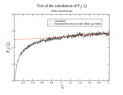
Figure 2: Non-perturbative calculation of the effective interaction $F_{2}(\xi)$ for a dilute instanton gas with $\alpha=7$, $m=1$, $\beta=1$ in a volume $T=200$. The points are the results obtained from projecting 1000 configurations, while the dashed line is the expected theoretical results for $\xi$ much larger than the instanton size (which is 0.26, in these units).

In order to show that our method yields the correct result, let us first consider a model for which the effective interaction can be evaluated analytically. The two-body part of the effective interaction for a dilute instanton gas can be easily computed from Eq. (30), by integrating out all the collective coordinates, except for those of a single instanton-antiinstanton pair. The result is

$$e^{-\frac{1}{\hbar}F_{2}^{IA}(\xi)}=\textrm{const.}\times e^{-(\kappa T-1)\log\left(T-\xi\right)},$$ (102)

This result holds for high barriers and distances $\xi$ much larger than the instanton size. Notice that, in the thermodynamic limit — $N,T\to\infty$ and $N/T=\kappa$ fixed— the effective interaction $F_{2}^{IA}(\xi)$ should scale linearly, with a slope controlled by the instanton rate $\kappa$.

We now address the question if our projection technique is able to reconstruct the effective interaction in Eq.(102). To this end, we have generated an ensemble of 1000 dilute gas configurations, by randomly sampling the positions of instantons and anti-instantons, in a box of size $T=200$ for a well with $\alpha=7,m=1,\beta=1$. In Fig. 2, we compare the expected theoretical curve (dashed line) with the result of our numerical calculation (points). We see that, as soon as the distance $\xi$ becomes larger than few instanton sizes —which is 0.26 in this units— the numerical results agree with the expected curve. A linear fit of the data for $\xi>1$ yields a slope of $0.32\pm 1$, in excellent agreement with the exact theoretical result, which is $0.31$. Hence, we conclude that our projection method is indeed able to quantitively reconstruct the structure of the exact distribution used to generate the ensemble of configurations.

Let us now discuss for completeness the structure of the effective interaction, for our original quantum double-well system. At this level, we no longer consider the semi-classical dilute gas model. Instead, we account for quantum fluctuations to all orders. As the barrier becomes higher and higher, performing a sampling of multiple barrier-crossing paths contributing to the functional integral with dynamical algorithms such as Molecular Dynamics of Monte Carlo becomes highly inefficient, and computationally expensive. To cope with this problem, we have evaluated the instanton-antiinstanton interactions using the importance sampling approach described in appendix A.

Fig. 3 shows the results of such a non-perturbative calculation for a well with $\alpha=1$ (low barrier) and $\alpha=7$ (high barrier). Some comments on these results are in order. First of all we note that the minimum of the effective interaction $F^{IA}_{2}(\xi)$ is located at positive values of $\xi$, in qualitative agreement with our perturbative calculation. The range of $\xi$ in which the effective interaction $F^{IA}_{2}(\xi)$ is not flat corresponds to close, largely overlapping instanton-antiinstanton pair configurations. When the distance becomes of the order of twice the instanton size, the effective interaction starts to raise and eventually reaches the dilute gas limit. On the other hand, for low barriers, the instanton density is large and the attraction and repulsion generated by $F^{IA}_{2}(\xi)$ become important. In such a regime, the vacuum behaves like a one-dimensional liquid, rather than as an ideal gas. We note that this is precisely the physical picture underlying the instanton liquid model of the vacuum fluct .

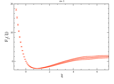
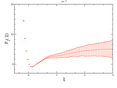
Figure 3: Non-perturbative calculation of the effective interaction $F(\xi)$ for $\alpha=1$ (left panel) and $\alpha=7$.

VII Conclusions

In this paper, we have presented an approach which allows to express quantum mechanical path integrals, in terms of few ordinary integrals over a set of low-energy variables, which parametrize the manifold of the relevant vacuum field configurations. We have developed a rigorous technique to extract the effective interaction, a simple quantum mechanical problem, in which the low-energy degrees of freedom are multi-instanton configurations.

We have assessed the accuracy of our method by correctly reconstructing the effective interaction used to generate an ensemble of sinthetic configurations. We have also performed both perturbative and non-perturbative calculation of the quantum effective interaction of an instanton-antiinstanton pair. In both cases, we have found that the effect of quantum fluctuations is to shift the location of the minimum of the effective interaction $F^{IA}_{2}(\xi)$ to the right.

We stress the fact that, although the present discussion has focused on an instanton liquid picture of the vacuum, our projection method does not rely at all on the semi-classical approximation. The semi-classical approximation has been used only as a guidance to find good vacuum effective degrees of freedom, for our toy model. Hence, the method can in principle be generalized to build effective theories for the vacuum, based on different types of field configurations. This observation may become important in QCD, where fields other than singular gauge instantons are needed, in order to account for confinement.

If the vacuum fields selected are the ones driving the system’s non-perturbative dynamics, then one expects that the contribution coming to the fluctuations around them to the field operators appearing in the Green’s functions will be small. In this case, the calculations of observables in the effective theory can be performed very efficiently, because they involve only few ordinary integrals over the set of curvilinear coordinates.

Most importantly, once a specific choice of the vacuum manifold has been identified, the corresponding effective theory yields parameter-free predictions. Hence, the present framework can be used to assess the importance of different families of vacuum fields, by directly comparing the results of the corresponding effective theory with the experimental data.

The extension of the present formalism to QCD is in progress and will be presented in our upcoming papers.

Appendix A Algorithm Used in the Evaluation of $F_{2}^{IA}(\xi)$

We are interested in computing numerically the integral

$$g^{IA}_{2}(\xi) = \mathcal{N}\leavevmode\nobreak\ \int\leavevmode\nobreak\ \mathcal{D}y\leavevmode\nobreak\ \exp\left\{-\int\leavevmode\nobreak\ \mbox{d}t\leavevmode\nobreak\ \mathcal{L}[\tilde{x}_{S_{2}}(t;\chi-\frac{1}{2}\xi,\chi+\frac{1}{2}\xi)+y(t)]\right\}\delta\bigg{(}y\cdot g_{\chi}\big{(}\bar{\chi},\bar{\xi}\big{)}\bigg{)}\delta\bigg{(}y\cdot g_{\xi}\big{(}\bar{\chi},\bar{\xi}\big{)}\bigg{)}\times$$ (103)

$$\!\!\!\!\!\!\!\!\!\!\!\!\!\!\!\!\!\!\!\!\!\!\!\!\!\!\!\!\!\!\times\bigg{[}\bigg{(}g_{\chi}\big{(}\chi,\xi\big{)}\cdot g_{\chi}\big{(}\bar{\chi},\bar{\xi}\big{)}\bigg{)}\bigg{(}g_{\xi}\big{(}\chi,\xi\big{)}\cdot g_{\xi}\big{(}\bar{\chi},\bar{\xi}\big{)}\bigg{)}-\bigg{(}g_{\chi}\big{(}\chi,\xi\big{)}\cdot g_{\xi}\big{(}\bar{\chi},\bar{\xi}\big{)}\bigg{)}\bigg{(}g_{\xi}\big{(}\chi,\xi\big{)}\cdot g_{\chi}\big{(}\bar{\chi},\bar{\xi}\big{)}\bigg{)}\bigg{]},$$

where the term inside the square brackets is the explicit representation of the Jacobian factor $\Phi[y]$.

The meta-stability of the double well system makes it rather computationally challenging to generate a statistically significative ensemble of field configurations, using algorithms based on Metropolis or by Langevin dynamics. The main problem is that, for such a meta-stable system, ergodicity is reached only in an exponentially large computational time.

The problem has no easy solution within a dynamical Monte Carlo approach. However, because of the low dimensionality of our system, simpler importance sampling technique are available and efficient. Since the system is time-translationally invariant, without loss of generality we can set $\chi=0$, $\bar{\chi}=0$ — i.e. we can remove completely the dependance from the center of mass—, and set $\bar{\xi}=0$. Then, the resulting expression for the pair correlation function can be re-written as

$$g^{IA}_{2}(\xi)=\mathcal{N}\int\mathcal{D}y\leavevmode\nobreak\ \delta(y(t)\cdot g_{\xi}(t;0))\leavevmode\nobreak\ \Phi[y]\leavevmode\nobreak\ \hat{P}[y(t)]\leavevmode\nobreak\ \frac{e^{-S\left[\tilde{x}_{S_{2}}\left(t,-\frac{1}{2}\xi,\frac{1}{2}\xi\right)+y(t)\right]}}{\hat{P}[y(t)]},$$ (104)

where $\hat{P}[y(t)]$ is a probability distribution to be defined below. We stress that now the integral can be restricted to the small region in which the projection function is not exponentially small. The discretized version of Eq. (104) is

$$g^{IA}_{2}(\xi)=\mathcal{N}\leavevmode\nobreak\ \int\prod_{k=1}^{N}\mbox{d}y(t_{k})\delta\left(\sum_{k=1}^{N}y(t_{k})g_{\xi}(t_{k},0)\right)\leavevmode\nobreak\ \Phi[y]\leavevmode\nobreak\ \hat{P}[y]\leavevmode\nobreak\ \frac{e^{-S_{\rm lat}\left[\tilde{x}_{S_{2}}\left(t_{k},-\frac{1}{2}\xi,\frac{1}{2}\xi\right)+y\right]}}{\hat{P}[y]},$$ (105)

where $N$ is the number of points in the lattice and $S_{\rm lat}$ is the discretised version of $S$.

For $\hat{P}[y]$ we choose:

$$\hat{P}[y]\propto\exp\left(-\frac{1}{8m\Delta t}\sum_{k=0}^{N}(y(t_{k+1})-y(t_{k}))^{2}\right)$$ (106)

with the constraint $y(t_{0})=y(t_{N+1})=0$. We eliminate the delta function by setting the last coordinate $y(t_{N})$ equal to

$$y(t_{N})=-\sum_{i=1}^{N-1}y(t_{i})g_{\xi}(t_{i})/g_{\xi}(t_{N}).$$ (107)

Notice that, in this way, the orthogonality condition is satisfied configuration by configurations. The statistical weight of resulting each paths was evaluated from

$$w_{i}(\xi)=\frac{\exp(-S_{\rm lat}[\tilde{x}_{s}(t_{k},\xi)+y_{i}])}{\hat{P}[y_{i}]}.$$ (108)

Up to an overall multiplicative factor, $g^{IA}(x)$ can be extracted from

$$g^{IA}_{2}(\xi)=\textrm{const.}\times\sum_{i}w_{i}(\xi)$$ (109)

By taking the logarithm, one obtains $F^{IA}_{2}(\xi)$, up to an overall additive constant.

References

(1) D.Diakonov, Lectures at the Enrico Fermi School in Physics, Varenna, June 27 – July 7, 1995. ArXiv:hep-ph/9602375v1.
(2) T. Schaefer and E. Shuryak, Rev. Mod. Phys. 70, 323
(1998).
(3) M. Cristoforetti, P. Faccioli, J.W.Negele and M. C. Traini, Phys. Rev. D 75 (2007), 034008. M. Cristoforetti, P. Faccioli, and M. C. Traini, Phys. Rev. D 75, (2007) 054024.
(4) P. Faccioli, A. Schwenk, and E. Shuryak, Phys. Lett. B 549, 93 (2002). P. Faccioli, Phys. Rev. C 69 (2004), 065211.
P. Faccioli, A. Schwenk, and E. Shuryak, Phys. Rev. D 67 (2003),
113009. M. Cristoforetti, P. Faccioli, E. Shuryak, and M. Traini, Phys. Rev. D 70 (2004), 054016 .
(5) A. Di Giacomo, AIP Conf.Proc.964 (2007), 348.
(6) R. Bertle, J. Greensite, S. Olejnik, "Quark Confinement and the Hadron Spectrum IV: Proceedings." ,
edited by Wolfgang Lucha and Khin Maung Maung, World Scientific, Singapore, 2002. ArXiv: hep-lat/0009017.
(7) F. Lenz , J.W. Negele , M. Thies, Phys. Rev. D69(2004), 074009.
(8) F. Lenz , J. W. Negele , M. Thies, Annals Phys. 323 (2008),1536.
(9) A. Laio and M. Parrinello, Proc. Nat. Acad. Sci 99 (2002),12563.
(10) D.I. Dyakonov and V.Yu Petrov, Nucl. Phys. B245(1984) 259.
(11) M.Hutter, Ph.D. Thesis, Ludwig Maximilians University Munich (1995), arXiv:hep-ph/0107098.
(12) Coleman, S., 1977, ”The uses of instantons”, Prooceedings of the 1977 School of Subnuclear Physics, Erice (Italy), reproduced in Aspects of Symmetry (Cambridge University Press, Cambridge, England, 1985), p. 265.
(13) E.V. Shuryak, Nucl. Phys. B302 (1988) 621
(14) G. Parisi, Yongshi Wu , Sci.Sin.24 (1981) 483
(15) Y. Grandati, A. Berard, P. Grange , Ann. of Phys. 246 2 (1996) 291
(16) M. Chu, J. Grandy, S. Huang, and J. W. Negele, Phys. Rev. D 49 (1994), 6039.
(17) D.Diakonov, and V. Yu Petrov, Nucl. Phys. B245 (1984) 259.