Mock LISA data challenge for the Galactic white dwarf binaries

Abstract

We present data analysis methods used in detection and the estimation of parameters of gravitational wave signals from the white dwarf binaries in the mock LISA data challenge. Our main focus is on the analysis of challenge 3.1, where the gravitational wave signals from more than $6\times 10^{7}$ Galactic binaries were added to the simulated Gaussian instrumental noise. Majority of the signals at low frequencies are not resolved individually. The confusion between the signals is strongly reduced at frequencies above 5 mHz. Our basic data analysis procedure is the maximum likelihood detection method. We filter the data through the template bank at the first step of the search, then we refine parameters using the Nelder-Mead algorithm, we remove the strongest signal found and we repeat the procedure. We detect reliably and estimate parameters accurately of more than ten thousand signals from white dwarf binaries.

I Introduction

The Galaxy contains a numerous population of the ultra-compact binaries which have orbital periods shorter than one hour. The observations of those binaries carry important astrophysical information about the internal stellar structure, formation of binaries and their evolution N09 . Due to the short period and proximity, the ultra-compact Galactic binaries will be an important source of gravitational waves (GW) for the future space borne interferometer LISA. LISA is planned to be launched in the next decade jointly by ESA and NASA. The bandwidth of the LISA detector is expected to be from 0.1 mHz to 100 mHz. In this frequency range we expect around $6\times 10^{7}$ ultra-compact binaries. These binaries will be dominated by the population of the white dwarf binaries. The number of the observed ultra-compact binaries will be so large below 3 mHz that they are not individually resolvable and form a cyclo-stationary background which dominates over the instrumental noise above 0.1 mHz ETK05 ; ETK05b . The number of binaries drops significantly above 7-8 mHz.

The most common sources are white-dwarf/white-dwarf binaries emitting gravitational wave signals of nearly constant frequency and amplitude. We also expect to observe few white-dwarf/neutron star binaries. The binaries could be of two major types:

(i) Detached, separated white-dwarf/white-dwarf binaries whose evolution is driven by radiation reaction. They are the end points of many binary evolution scenarios. The gravitational wave carry information about the mass of the binary and the distance.

(ii) Interacting binaries. Those are close systems with a significant tidal interaction and/or with the Roche lobe overflow. In those systems the gravitational radiation reaction competes against mass transfer and the orbital period can either increase or decrease. Currently there are 22 known accreting binaries, so called AM CVn stars, with periods between 5.4 and 65 min N09b . The radiation from those binaries fall into the LISA band and they will serve as verification binaries SV06 .

It was demonstrated rep:mldc2 that one can detect and remove a few tens of thousand of those signals. The resolved systems will provide the map of the compact binaries in the Galaxy and will allow us to constrain the evolutionary pathways of those systems.

A series of mock LISA data challenges (MLDC) was organized in order to foster development of LISA data analysis algorithms and to compare the performance of different methods web:mldc ; over:mldc1 ; rep:mldc1 ; over:mldc2 . The simulated Galaxy consists of only white dwarf binaries (of both types detached and interacting) in circular orbit and it is based on the population synthesis described in N01 ; N04 . It is expected that white dwarf binaries will largely dominate over more heavy binaries like neutron stars and/or black holes. Eccentric white dwarf binaries could be generated in globular clusters but their number is a tiny fraction of the total population B01 ; W07 . The gravitational wave signals produced by white dwarf Galactic binaries span the whole LISA band, they stand above the instrumental noise starting at 0.1 mHz and propagate all the way up to few tens of mHz.

Let us give a brief overview of currently available methods. The fully coherent methods employing matched filtering techniques can be split in two groups: stochastic search and grid-based search.

The stochastic search does not map uniformly the whole parameter space, instead it concentrates on the regions with high likelihood. The first type of the stochastic search is suggested in CCR07 and it is based on the genetic algorithm. The genetic algorithm is an optimization method which evolves the set of templates (a colony of organisms) in the direction of increasing likelihood (improving fitness of organisms) using a certain rules (selection, breeding, mutation). Another stochastic method is based on constructing the (Markov) chains using Metropolis-Hastings acceptance/rejection rule. The Bayesian methods are powerful tools to get posterior probability distribution function. A pure MCMC (Markov chain Monte-Carlo) algorithm does not perform well due to presence of quite strong (and well separated in the parameter space) secondary maxima in the likelihood. Two currently available Bayesian algorithms differ mainly in the way they explore the parameter space. BAM algorithm suggested in C2 uses multiple proposal distributions reflecting possible correlations in the parameter space in combination with the simulated annealing. At the search stage (the search for the global maximum in the parameter space) the Markovian properties of the chain are quite often not respected, and, once the search is completed, the sampling stage starts during which the classical MCMC algorithm is used. The key feature of BAM is blocking: the search is conducted in the several frequency bands each split in several small blocks. The algorithm steps through these blocks updating all sources within a given band simultaneously. After all blocks have been updated, they are shifted by one-half the width of a blocks for the next round of updates to eliminate boundary effect. The results from the different frequency bands are glued together using the overlapped buffer zones. Another MCMC-based method is described in TVV . The authors suggest to use delayed rejection MCMC to explore the parameter space, find the global maximum and sample the posterior distribution. The basic idea behind ”delayed rejection” is an extended acceptance/rejection rule: we allow several jumps before rejecting/accepting the next point in the chain, and each following trial jump learns the property of the parameter space explored by the previous jumps. An additional advantage of the ”delayed rejection” is that the variance of an estimate made from a chain using delayed rejection is always smaller than that produced with a standard Markov chain.

The grid-based search maps the whole parameter space by computing the (log) likelihood (usually in the form of $\mathcal{F}$-statistic) on the uniformly distributed grid points (often referred as a template bank). A particular implementation of this method is presented in this paper. Another version of the grid based method is described in WPK . There the authors adopt the software used for searching continuous GW signals in the LIGO/VIRGO/GEO600 data to construct the grid in the parameter space (in four Doppler parameters: sky location, frequency of GW signals and its derivative at some fiducial time) and to compute $\mathcal{F}$- statistic. Besides that, the authors in WPK attempt to detect several signals at once while we are dealing with one (the strongest) signal at the time. They separate the secondary maxima from the primary by requiring the coincidence in the parameters recovered from the analysis of different time delay interferometry (TDI) streams (for more information on TDI, see TD and references therein). Once the prime maxima are identified, the grid mesh is refined by zooming in onto them to improve the parameter estimation. The detected signals are removed from the data and the procedure is repeated.

The last type of search uses Radon transform to identify the frequency of the signal and the source’s sky location MN . The basis of this method is that the LISA response function can be seen as a Radon transform of binary distribution in those three parameters.

Galactic binaries were present in all four challenges conducted so far. In this article we report our results of the analysis of challenge 3.1 data set. This data set contains approximately $6\times 10^{7}$ Galactic binaries with simulated instrumental noise. The GW signals had measurable frequency evolution at high frequencies. The participants of the challenge have returned the parameters of the detected signals: the sky position in ecliptic coordinates, frequency of GW and its first derivative, inclination of the orbit to the line of sight, polarization angle, initial GW phase and the amplitude.

The paper is organized as follows. In Section 2 we shall present an analytic approximation to the response of the LISA detector to a gravitational wave signal from a binary system. We shall not give details of the derivation, these can be found in the original papers AET99 , CR03 , and KTV04 . In Section 3 we shall present the maximum likelihood method in application to detection and estimation of parameters of the GW signal from a binary system imbedded in stationary Gaussian noise. In Section 4 we describe our data analysis tools and algorithms that we have implemented our computer codes for challenge 3.1 search. We describe the search strategy in Section 5 and discuss the results of the search in Section 6.

II Response of the LISA detector to the gravitational-wave signal from a binary system

The LISA detector consists of 3 satellites forming a constellation of an approximately equilateral triangle. The constellation rotates around the Sun with a period of 1 year trailing the Earth by 20 degrees. The triangular constellation is inclined at 60 degrees to the ecliptic and rotates itself around its center with a period of 1 year in the direction opposite to the rotation around the Sun. The LISA detector in general will produce 3 independent data streams. In the long wavelength approximation, when the length of the gravitational wave is much longer than the distance between the spacecraft, the number of independent data streams degenerates into 2. There are various combinations of the responses of the LISA detector (see AET99 for details). The data simulated for the mock LISA data challenge are the first-generation TDI Michelson combinations that we denote by X, Y, and Z. TDI is a software technique (AET99 ) by which we remove the dominant frequency noise from the LISA instrumental noise, first generation means that in the TDI procedure we assume that the distances between the spacecraft are constant, independent of time. In this Section we shall summarize approximate analytic formulas for the first TDI generation Michelson responses of the LISA detector to a gravitational wave signal from a binary system. The formulas are essentially the same as in Appendix C KTV04 except that they are given using the conventions used in the Synthetic LISA numerical software V05 . The GW response of the first-generation TDI Michelson observable $X$ is given by a linear combination of the four time-dependent functions $X^{(k)}(t)$.

$$X(t)=2\,\omega L\,\sin(\omega L)\sum_{k=1}^{4}a^{(k)}X^{(k)}(t),$$ (1)

where $\omega$ is the angular gravitational wave frequency and $L$ is the distance between the spacecrafts of the LISA detector.

Before we give functions $X^{(k)}(t)$ let us introduce few notations. First we define the polarization basis in the solar system barycenter frame (following how:mldc ):

$$\hat{u} = \{\sin(\beta),\cos(\lambda),\sin(\beta)\}\sim\frac{\partial\hat{k}}{\partial\beta}$$ (2)

$$\hat{v} = \{\sin(\lambda),-\cos(\lambda),0\}\sim\frac{\partial\hat{k}}{\partial\lambda},$$ (3)

where $\beta$ and $\lambda$ are, respectively, the latitude and the longitude of the source in ecliptic coordinates and $\hat{k}=-\{\cos(\beta)\cos(\lambda),\cos(\beta)\sin(\lambda),\sin(\beta)\}$ is direction of the wave propagation. Then we introduce the LISA motion used in the production of MLDC data. The position of each spacecraft can be split in the position of the guiding center $\vec{R}$ and position of the spacecraft with respect to that center:

$$\vec{r}_{i}=\vec{R}+L\vec{q}_{i},\quad i=1,2,3,$$ (4)

here we have assumed LISA to be a rigid equilateral triangle: $L=L_{1}=L_{2}=L_{3}$, and the $\vec{q}_{i}$ are as follows

$$\vec{q}_{i}=\frac{1}{2\sqrt{12}}\left\{\cos(2\Omega t-\chi_{i})-3\cos(\chi_{i}),\sin(2\Omega t-\chi_{i})-3\sin(\chi_{i}),-\sqrt{12}\cos(\Omega t-\chi_{i})\right\},$$ (5)

where $\chi_{i}=2(i-1)\pi/3$. The unit vectors along the arms can be defined via vectors $\vec{q}_{i}$: $\hat{n}_{1}=\vec{q}_{2}-\vec{q}_{3}$, and others are obtained by cyclic permutation of indices: $1\to 2\to 3\to 1$. Now we are ready to write $X^{(k)}$:

$$\left[\!\begin{array}[]{c}X^{(1)}\\ X^{(2)}\end{array}\!\right]=\left[\!\begin{array}[]{c}u_{2}(t)\\ v_{2}(t)\end{array}\!\right]\!\bigl{\{}\mbox{sinc}\bigl{[}(1+\hat{k}\hat{n}_{2})x/2\bigr{]}\cos\bigl{[}\phi(t)+(x/2)\hat{k}\vec{q}_{2}-3x/2\bigr{]}$$ (8)

$$\hskip 82.51299pt+\hskip 4.2679pt\mbox{sinc}\bigl{[}(1-\hat{k}\hat{n}_{2})x/2\bigr{]}\cos\bigl{[}\phi(t)+(x/2)\hat{k}\vec{q}_{2}-5x/2\bigr{]}\bigr{\}}$$

$$\hskip 39.83385pt-\left[\!\begin{array}[]{c}u_{3}(t)\\ v_{3}(t)\end{array}\!\right]\!\bigl{\{}\mbox{sinc}\bigl{[}(1+\hat{k}\vec{n}_{3})x/2\bigr{]}\cos\bigl{[}\phi(t)+(x/2)\hat{k}\vec{q}_{3}-5x/2\bigr{]}$$ (10)

$$\hskip 82.51299pt+\hskip 4.2679pt\mbox{sinc}\bigl{[}(1-\hat{k}\vec{n}_{3})x/2\bigr{]}\cos\bigl{[}\phi(t)+(x/2)\hat{k}\vec{q}_{3}-3x/2\bigr{]}\bigr{\}}$$ (11)

and $X^{(3)}$, $X^{(4)}$ are obtained by replacing $\cos$ with $\sin$ in $X^{(1)}$ and $X^{(2)}$ respectively. In the above equation we have used:

$$u_{i} = -\frac{1}{2}\left[(\hat{u}\hat{n}_{i})^{2}-(\hat{v}\hat{n}_{i})^{2}\right]$$ (12)

$$v_{i} = (\hat{u}\hat{n}_{i})(\hat{v}\hat{n}_{i}),$$ (13)

where $x=\omega L$ and ${\mathrm{sinc}(\ldots)}\,=\frac{\sin{(\ldots)}}{(\ldots)}$. The GW responses for $Y$ and $Z$ can be obtained by cyclical permutation of the spacecraft indices.

The phase modulation function $\phi(t)$ is given by

$$\phi(t)=\omega t+\frac{1}{2}\dot{\omega}t^{2}+(\omega+\dot{\omega}t)\,R\cos\beta\cos(\Omega t+\eta_{o}-\lambda),$$ (14)

where $\Omega=2\pi/1$year, $\eta_{o}$ is the position of the constellation on the orbit around the Sun at time $t=0$, and $R$ is $1$ astronomical unit. The small eccentricity of the Earth orbit (e = 0.017) can be neglected because it contributes less than one cycle to the phase $\phi(t)$ above for gravitational wave frequencies from 0.1 mHz to 12 mHz for which we analyze the data. The parameter $\dot{\omega}$ is the frequency drift which may occur either due to the gravitational radiation reaction or as a result of the tidal interaction between the components of the binary system. In the case of a detached binary system evolving only due to the gravitational radiation reaction the frequency drift $\dot{\omega}$ is approximately given by (see Section IID of KTV04 for discussion).

$$\dot{\omega}=\frac{48}{5}\left(\frac{G{\cal M}_{c}}{2c^{3}}\right)^{5/3}\!\!\!\omega^{11/3},$$ (15)

where $\mathcal{M}_{c}=m_{1}^{3/5}m_{2}^{3/5}/(m_{1}+m_{2})^{1/5}$ is the chirp mass ($m_{1}$ and $m_{2}$ are the individual masses of the components of the binary).

Finally the constant amplitudes $a^{(k)}$ take the form

$$a^{(1)} = \ h_{0}^{+}\cos\phi_{0}\,\cos 2\psi-h_{0}^{\times}\sin\phi_{0}\,\sin 2\psi,$$ (16)

$$a^{(2)} = \ h_{0}^{+}\cos\phi_{0}\,\sin 2\psi+h_{0}^{\times}\sin\phi_{0}\,\cos 2\psi,$$ (17)

$$a^{(3)} =- \ h_{0}^{+}\sin\phi_{0}\,\cos 2\psi-h_{0}^{\times}\cos\phi_{0}\,\sin 2\psi,$$ (18)

$$a^{(4)} =- \ h_{0}^{+}\sin\phi_{0}\,\sin 2\psi+h_{0}^{\times}\cos\phi_{0}\,\cos 2\psi,$$ (19)

where

$$h_{0}^{+} = h_{0}(1+\cos^{2}\iota)/2,$$ (20)

$$h_{0}^{\times} = h_{0}\cos\iota.$$ (21)

The parameters $h_{0}$, $\phi_{0}$, $\psi$, and $\iota$ are constant amplitude, the constant phase of the signal, the polarization angle, and the inclination angle respectively. In the case of a detached binary system evolving only due to the gravitational radiation reaction the constant amplitude $h_{0}$ is given by

$$h_{0}=\frac{4(G\mathcal{M}_{c})^{5/3}}{c^{4}D_{L}}\left[\frac{\omega}{2}\right]^{2/3}\!\!,$$ (22)

where $D_{L}$ is the luminosity distance to the source.

One can invert the equations (16) for amplitudes to obtain formulas for astrophysical parameters $h_{0}$, $\phi_{0}$, $\psi$, and $\iota$. We first introduce the quantities

$$A = (a^{(1)})^{2}+(a^{(2)})^{2}+(a^{(3)})^{2}+(a^{(4)})^{2},$$ (23)

$$D = a^{(1)}a^{(4)}-a^{(2)}a^{(3)}.$$ (24)

Then the constants $h_{0}^{+}$, $h_{0}^{+}$, $h_{0}$, and $\phi_{0}$ can be uniquely determined.

$$h_{0}^{+} = \sqrt{(A+\sqrt{A^{2}-4D^{2}})/2},$$ (25)

$$h_{0}^{\times} = \mbox{sign}(D)\sqrt{(A-\sqrt{A^{2}-4D^{2}})/2},$$ (26)

$$h_{0} = h_{0}^{+}+\sqrt{h_{0}^{+2}-h_{0}^{\times 2}},$$ (27)

$$\iota = \mbox{acos}(h_{0}^{\times}/h_{0}).$$ (28)

Finally the constant phase $\phi_{0}$ and the polarization angle $\psi$ can be obtained from the following equations:

$$\tan 2\phi_{0} = \frac{2(a^{(1)}a^{(3)}+a^{(2)}a^{(4)})}{(a^{(3)})^{2}+(a^{(4)})^{2}-(a^{(1)})^{2}-(a^{(2)})^{2}},$$ (29)

$$\tan 4\psi = \frac{2(a^{(1)}a^{(2)}+a^{(3)}a^{(4)})}{(a^{(1)})^{2}+(a^{(3)})^{2}-(a^{(2)})^{2}-(a^{(4)})^{2}}.$$ (30)

The long-wavelength (LW) approximation to the GW responses is obtained by taking the leading-order terms of the generic expressions in the limit of $\omega L\rightarrow 0$:

$$X_{LW}(t) \simeq 4(\omega L)^{2}\{[u_{2}(t)-u_{3}(t)]\left[a^{(1)}\cos\phi(t)+a^{(3)}\sin\phi(t)\right]$$ (32)

$$+[v_{2}(t)-v_{3}(t)]\left[a^{(2)}\cos\phi(t)+a^{(4)}\sin\phi(t)\right]\}$$

and $Y_{LW}$, $Z_{LW}$ responses are obtained by cyclical permutation of the indices.

In Fig. 1 we have compared the power spectra of the signal generated using the analytic formulas given above by equation (1) with the power spectrum of noise free response generated by Synthetic LISA software for one of the training sets provided in MLDC. Synthetic LISA software was used to generate the analyzed MLDC data sets.

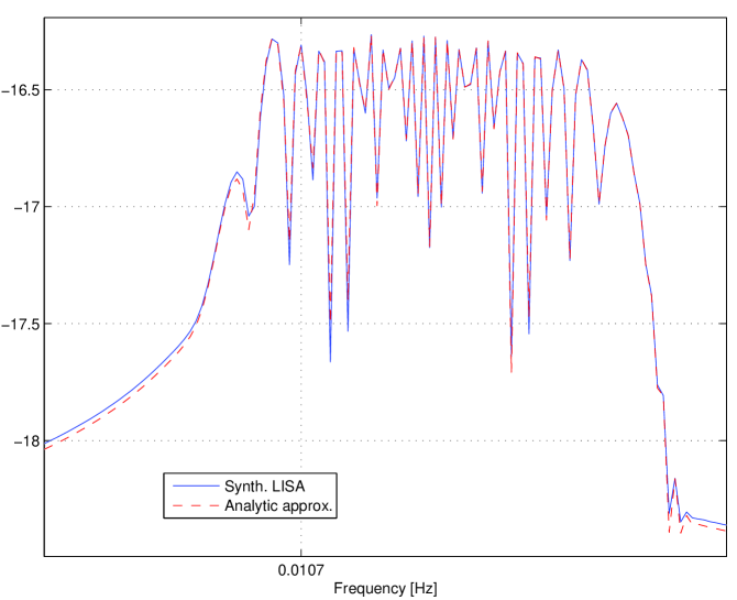
Figure 1: Comparison of the power spectra of the gravitational-wave signal response using the analytic formulas presented in this paper and Synthetic LISA V05 .

III Maximum likelihood detection and parameter estimation

To detect the signal and estimate its parameters we use the maximum likelihood (ML) estimation method which consists of maximizing the likelihood function $\Lambda$ with respect to the parameters of the signal W71 . Let us first consider the Michelson $X$ combination given in the previous section. We assume that the noise in the detector is a stationary Gaussian random process. Moreover we assume that over the bandwidth of the signal the spectral density of the noise is approximately constant and equal to $S_{o}=S(\omega_{o})$. This condition should be well fulfilled for the case of a gravitational wave signal from a white dwarf binary in LISA detector noise. Then we can approximate the log likelihood function by

$$\log\Lambda=2\,\frac{T_{o}}{S_{o}}[{\langle y^{X}X\rangle}-\frac{1}{2}{\langle X^{2}\rangle}],$$ (33)

where $y^{X}$, is the noisy data in the $X$ channel, $S_{o}$ is one-sided spectral density of the noise, $T_{o}$ is the observation time, and the time-averaging operator ${\langle\cdot\rangle}$ is defined by

$${\langle g\rangle}:=\frac{1}{T_{o}}\int^{T_{o}}_{0}g(t)\,dt.$$ (34)

By introducing the variables

$$h^{(k)}=2\,\omega L\,\sin(\omega L)X^{(k)}$$ (35)

the $X$ combination can be written in a compact form

$$X=\sum_{k=1}^{4}a^{(k)}h^{(k)}.$$ (36)

The ML estimators $\hat{a}^{(k)}$ of the amplitudes are found by maximizing $\log\Lambda$ with respect to parameters $a^{(k)}$, that is by solving

$$\frac{\partial\log\Lambda}{\partial a^{(k)}}=0.$$ (37)

The equations (37) above are equivalent to the following set of linear equations

$$\sum_{k=1}^{4}M^{(l)(k)}a^{(k)}=N^{(l)},\quad l=1,\ldots,4,$$ (38)

where

$$M^{(l)(k)} = {\langle h^{(k)}\,h^{(l)}\rangle},$$ (39)

$$N^{(l)} = {\langle y^{X}\,h^{(l)}\rangle}.$$ (40)

Thus the maximum likelihood estimators $\hat{a}^{(k)}$ of the amplitudes are explicitly given by

$$\hat{a}^{(k)}=\sum_{l=1}^{4}\big{(}M^{-1}\big{)}^{(l)(k)}N^{(l)}.$$ (41)

Substituting the above estimators $\hat{a}^{(k)}$ for amplitudes $a^{(k)}$ in the log likelihood function log$\Lambda$ yields the reduced log likelihood function that we denote by $\mathcal{F}$:

$$\mathcal{F}={\textstyle\frac{T_{o}}{S_{o}}}\sum_{l=1}^{4}\sum_{k=1}^{4}\big{(}M^{-1}\big{)}^{(l)(k)}N^{(l)}N^{(k)}.$$ (42)

We call the above function the $\mathcal{F}$-statistic.

One can show that the following relations hold approximately for the components of the matrix $M^{(l)(k)}$

$${\langle h^{(1)}\,h^{(3)}\rangle} = {\langle h^{(2)}\,h^{(4)}\rangle}=0,$$ (43)

$${\langle h^{(1)}\,h^{(1)}\rangle} = {\langle h^{(3)}\,h^{(3)}\rangle},$$ (44)

$${\langle h^{(2)}\,h^{(2)}\rangle} = {\langle h^{(4)}\,h^{(4)}\rangle},$$ (45)

$${\langle h^{(1)}\,h^{(2)}\rangle} = {\langle h^{(3)}\,h^{(4)}\rangle},$$ (46)

$${\langle h^{(1)}\,h^{(4)}\rangle} = -{\langle h^{(2)}\,h^{(3)}\rangle}.$$ (47)

It is convenient to introduce the following variables

$$U=2{\langle h^{(1)}\,h^{(1)}\rangle},$$ (48)

$$V=2{\langle h^{(2)}\,h^{(2)}\rangle},$$ (49)

$$Q=2{\langle h^{(1)}\,h^{(2)}\rangle},$$ (50)

$$P=2{\langle h^{(1)}\,h^{(4)}\rangle}.$$ (51)

Let us introduce the complex amplitude parameters

$$a^{(u)} = a^{(1)}+ia^{(3)},$$ (52)

$$a^{(v)} = a^{(2)}+ia^{(4)},$$ (53)

where $a^{(k)}$ are given by Eqs. (16)–(19). Let us also define the complex modulation functions $m^{(u)}$ and $m^{(v)}$ by

$$\begin{split}\left[\!\begin{array}[]{c}m^{(u)}\\ m^{(v)}\end{array}\!\right]=&\left[\!\begin{array}[]{c}u_{2}(t)\\ v_{2}(t)\end{array}\!\right]\!\bigl{\{}\mbox{sinc}\bigl{[}(1+\hat{k}\vec{n}_{2})x/2\bigr{]}\exp i\bigl{[}(x/2)\hat{k}\vec{q}_{2}-3x/2\bigr{]}\\ &\quad\quad\quad\quad+\mbox{sinc}\bigl{[}(1-\hat{k}\vec{n}_{2})x/2\bigr{]}\exp i\bigl{[}(x/2)\hat{k}\vec{q}_{2}-5x/2\bigr{]}\bigr{\}}-\\ &\left[\!\begin{array}[]{c}u_{3}(t)\\ v_{3}(t)\end{array}\!\right]\!\bigl{\{}\mbox{sinc}\bigl{[}(1++\hat{k}\vec{n}_{3})x/2\bigr{]}\exp i\bigl{[}(x/2)\hat{k}\vec{q}_{3}-5x/2\bigr{]}\\ &\quad\quad\quad\quad+\mbox{sinc}\bigl{[}(1-\hat{k}\vec{n}_{3})x/2\bigr{]}\exp i\bigl{[}(x/2)\hat{k}\vec{q}_{3}-3x/2\bigr{]}\bigr{\}}.\end{split}$$ (54)

Introducing further complex quantities

$$W = Q+iP,$$ (55)

$$N^{(u)} = N^{(1)}+iN^{(3)},$$ (56)

$$N^{(v)} = N^{(2)}+iN^{(4)},$$ (57)

where $N^{(k)}$, $Q$ and $P$ are given by Eqs. (40), (50), and (51) respectively and using the approximate relations given by Eqs.  (43), (44), (45), (46), and (47)) we can write the ML amplitude estimators of the complex amplitudes and the ${\mathcal{F}}$-statistic in the following compact form

$$\left(\begin{array}[]{c}\hat{a}^{(u)}\\ \hat{a}^{(v)}\end{array}\right)=\frac{2}{\Delta}\left(\begin{array}[]{cc}V&-W^{*}\\ -W&U\end{array}\right)\cdot\left(\begin{array}[]{c}N^{(u)}\\ N^{(v)}\end{array}\right),$$ (58)

$${\mathcal{F}}=2\frac{T_{o}}{S_{o}}\frac{\left\{V\bigl{|}N^{(u)}\bigr{|}^{2}+U\bigl{|}N^{(v)}\bigr{|}^{2}-2\,\mathrm{Re}\left[W\,N^{(u)}(N^{(v)})^{*}\right]\right\}}{\Delta}.$$ (59)

where $\Delta=UV-|W|^{2}$. The integrals $N^{(u)}$ and $N^{(v)}$ can be expressed as

$$N^{(u)} = 2\,\omega L\,\sin(\omega L){\langle y^{X}(t)\,m^{(u)}(t)\,\exp i\phi(t)\rangle},$$ (60)

$$N^{(v)} = 2\,\omega L\,\sin(\omega L){\langle y^{X}(t)\,m^{(v)}(t)\,\exp i\phi(t)\rangle}.$$ (61)

As we shall see in the next section the above form of the $\mathcal{F}$-statistic is very suitable for a numerical implementation. In a similar manner one can derive the ${\mathcal{F}}$-statistic for other Michelson variables.

In order to extract information about the signal from all three independent variables we need to derive the ${\mathcal{F}}$-statistic for the whole LISA network. It is then useful to consider the so called ”optimal” combinations of the responses. These combinations have the property that their instrumental noises are uncorrelated (see P02 ) and consequently their cross-spectrum matrix is diagonal. In this case the log likelihood function for the whole network is the sum of log likelihood functions for the individual combinations, For the Michelson variables the optimal combination are given by optimal

$$A = \frac{Z-X}{\sqrt{2}},$$ (62)

$$E = \frac{X-2Y+Z}{\sqrt{6}},$$ (63)

$$T = \frac{X+Y+Z}{\sqrt{3}}.$$ (64)

The noisy data, $y^{A},y^{E}$ and $y^{T}$ are obtained as the analogous combination of the Michelson observables $y^{X},y^{Y}$ and $y^{Z}$, where $y^{Y}$, $y^{Z}$ are data in the $Y$ and $Z$ channels respectively. The log likelihood function for the network takes the form

$$\begin{split}\log{\cal L}=2\,T_{o}&\left\{\frac{1}{S_{A}(\omega_{o})}[{\langle y^{A}A\rangle}-\frac{1}{2}{\langle A^{2}\rangle}]+\right.\\ &\frac{1}{S_{E}(\omega_{o})}[{\langle y^{E}E\rangle}-\frac{1}{2}{\langle E^{2}\rangle}]+\left.\frac{1}{S_{T}(\omega_{o})}[{\langle y^{T}T\rangle}-\frac{1}{2}{\langle T^{2}\rangle}]\right\}.\end{split}$$ (65)

The power spectral densities $S_{A},S_{E},S_{T}$ are given by

$$\begin{array}[]{rcl}S_{A}(\omega)&=&S_{E}(\omega)=32\cos{(\omega L/2)}^{2}\sin{(\omega L/2)}^{2}\left\{[6+4\cos{(\omega L)}+\right.\\ &&\left.2\cos{(2\omega L)}]S^{pm}+[2+\cos{(\omega L)}]S^{op}\right\}\\ S_{T}(\omega)&=&128\cos{(\omega L/2)}^{2}\sin{(\omega L/2)}^{4}\left[4\sin{(\omega L/2)}^{2}S^{pm}+S^{op}\right],\end{array}$$ (66)

where $S^{\rm pm}$ and $S^{\rm op}$ are spectral densities of proof-mass noise and optical path noise respectively. It turns out that the ML estimators of the amplitudes and the ${\mathcal{F}}$-statistic can be written in the same form as for a single detector. To do this we introduce the following noise-weighted average procedure. For any two vectorial quantities ${\bf p}$ and ${\bf q}$,

$$\begin{array}[]{rcl}{\bf p}(t)&=&\left(p^{A}(t),p^{E}(t),p^{T}(t)\right),\\ \quad{\bf q}(t)&=&\left(q^{A}(t),q^{E}(t),q^{T}(t)\right),\end{array}$$ (67)

the noise-weighted average operator ${\langle\cdot\rangle}_{\cal S}$ is defined as follows,

$${\langle{\bf p}\,{\bf q}\rangle}_{\cal S}:=w_{A}\,{\langle p^{A}\,q^{A}\rangle}+w_{E}\,{\langle p^{E}\,q^{E}\rangle}+w_{T}\,{\langle p^{T}\,q^{T}\rangle},$$ (68)

where the weights $w_{I}$ ($I=A,E,T$) are defined by

$$w_{I}:=\frac{S^{-1}_{I}}{{\cal S}^{-1}},\quad I=A,E,T,\quad\text{with}\quad{\cal S}^{-1}=S_{A}^{-1}+S_{E}^{-1}+S_{T}^{-1}.$$ (69)

With the above definitions the log likelihood function of Eq. (65) defined for data
${\bf y}=(y^{A},y^{E},y^{T})$ and response ${\bf R}=(A,E,T)$ can be written in a compact form

$$\log{\cal L}=2\,\frac{T_{o}}{{\cal S}(\omega_{o})}[{\langle{\bf y}{\bf R}\rangle}_{\cal S}-\frac{1}{2}{\langle{\bf R}^{2}\rangle}_{\cal S}].$$ (70)

Having now defined ${\bf h}^{(k)}$ by [see Eq. (36)]

$${\bf R}=\sum_{k=1}^{4}a^{(k)}{\bf h}^{(k)}$$ (71)

and ${\cal M}^{(k)(l)},\;{\cal N}^{(l)}$ by [see Eqs. (39),(40)]

$${\cal M}^{(k)(l)} = {\langle{\bf h}^{(k)}\,{\bf h}^{(l)}\rangle}_{\cal S},$$ (72)

$${\cal N}^{(l)} = {\langle{\bf y}\,{\bf h}^{(l)}\rangle}_{\cal S}.$$ (73)

it is straightforward to get the maximum likelihood estimators of the complex amplitudes and the ${\mathcal{F}}$-statistic for the LISA network

$$\left(\begin{array}[]{c}\hat{a}^{(u)}_{opt}\\ \hat{a}^{(v)}_{opt}\end{array}\right)=\frac{2}{{\sf\Delta}}\left(\begin{array}[]{cc}{\sf V}&-{\sf W}^{*}\\ -{\sf W}&{\sf U}\end{array}\right)\cdot\left(\begin{array}[]{c}\mathcal{N}^{(u)}\\ \mathcal{N}^{(v)}\end{array}\right),$$ (74)

$${\mathcal{F}}_{opt}=2\frac{T_{o}}{\cal S}\frac{\left\{{\sf V}\bigl{|}\mathcal{N}^{(u)}\bigr{|}^{2}+{\sf U}\bigl{|}\mathcal{N}^{(v)}\bigr{|}^{2}-2\,\mathrm{Re}\left[{\sf W}\,\mathcal{N}^{(u)}(\mathcal{N}^{(v)})^{*}\right]\right\}}{{\sf\Delta}},$$ (75)

where ${\sf\Delta}={\sf U}{\sf V}-|{\sf W}|^{2}$ and $\sf W=\sf Q+i\sf P$. The quantities ${\sf V}$, ${\sf U}$, ${\sf Q}$, $\sf P$ in Eqs. (74) and (75) above are defined in the same way as quantities $V,U,Q,P$ in Eqs. (48)–(51), but with the time-averaging operator ${\langle\cdot\rangle}$ replaced everywhere by noise-weighted averaging operator ${\langle\cdot\rangle}_{S}$ and scalar functions $h^{(k)}$ by their vectorial counterparts ${\bf h}^{(k)}$. The two functions ${\cal N}^{(u)}$ and ${\cal N}^{(v)}$ are explicitly given by

$$\begin{array}[]{rcll}{\cal N}^{(u)}&=&{\cal N}^{(1)}+i{\cal N}^{(3)}&=2\,\omega L\,\sin(\omega L){\langle{\bf y}(t)\,{\bf m}^{(u)}(t)\,\exp i\phi(t)\rangle}_{\cal S},\\ {\cal N}^{(v)}&=&{\cal N}^{(2)}+i{\cal N}^{(4)}&=2\,\omega L\,\sin(\omega L){\langle{\bf y}(t)\,{\bf m}^{(v)}(t)\,\exp i\phi(t)\rangle}_{\cal S},\end{array}$$

where two vector functions ${\bf m}^{(u)}$ and ${\bf m}^{(v)}$ are the relevant combinations of $m^{(u)}$’s and $m^{(v)}$’s defined for $X$, $Y$ and $Z$ [see Eq. (54)].

IV Data analysis algorithms

IV.1 Use of the FFT algorithm

The detection statistic, $\mathcal{F}$ [Eq. (59) or (75)], involves integrals $N^{(u)}$ and $N^{(v)}$ of the form

$${\cal I}=\int^{T_{0}}_{0}y(t)\,m(t;\omega,\beta,\lambda)\,\exp[i\phi_{\mathrm{mod}}(t;\omega,\dot{\omega},\beta,\lambda)]\exp[i\omega t]\,dt$$ (76)

where $m$ is one of the two complex modulation functions (54), while the phase modulation $\phi_{\mathrm{mod}}$ is given by

$$\phi_{\mathrm{mod}}(t;\omega,\beta,\lambda)=\frac{1}{2}\dot{\omega}t^{2}+\omega R\cos\beta\cos(\Omega t+\eta_{0}-\lambda)$$ (77)

[see Eq. (14)]. In order to evaluate the integral (76) efficiently we would like to use the FFT algorithm. The integral (76) is not a Fourier transform because both the phase modulation function $\phi_{\mathrm{mod}}$ and the amplitude modulation function $m$ depend on the angular frequency $\omega$. We overcome these problems in the following way. Firstly we introduce a new representation of the phase, namely we introduce two new parameters

$$A=\omega R\cos\beta\cos(\lambda-\eta_{0}),$$

$$B=\omega R\cos\beta\sin(\lambda-\eta_{0}).$$ (78)

In this new parametrization the phase modulation takes the form

$$\phi_{\mathrm{mod}}(t;\dot{\omega},A,B)=\frac{1}{2}\dot{\omega}t^{2}+A\cos(\Omega t)+B\sin(\Omega t),$$ (79)

and it is independent of the angular frequency parameter $\omega$. A similar parametrization has been used in the search of the resonant bar NAUTILUS detector detector data for gravitational waves from spinning neutron stars (see ABJK02 ). (As we shall see in the following section the above parametrization by the coordinates $\{\omega,\dot{\omega},A,B\}$ will also prove useful in the construction of our grid.) Secondly we assume that the bandwidth $[\omega_{1}\,\omega_{2}]$ of the data is small so that the amplitude modulation function $m$ varies little over the interval of angular frequency from lower edge of the band $\omega_{1}$ to the upper edge of the band $\omega_{2}$. In order to satisfy the above approximation, in our search we have divided the data into narrow bands of $\Delta f\equiv(\omega_{2}-\omega_{1})/(2\pi)=0.1$ mHz by passing them through narrowband filters (see Section V for details) and each narrow-banded data were analyzed separately. Then we can approximate the modulation function $m(t;\omega,\beta,\lambda)$ by $m(t;\omega_{\mathrm{mid}},A,B)=m(t;\omega_{\mathrm{mid}},\beta_{\mathrm{mid}}(A,B,\omega_{\mathrm{mid}}),\lambda_{\mathrm{mid}}(A,B,\omega_{\mathrm{mid}}))$ where $\omega_{\mathrm{mid}}=(\omega_{2}-\omega_{1})/2$ and where $\beta_{\mathrm{mid}}(A,B,\omega_{\mathrm{mid}})$ and $\lambda_{\mathrm{mid}}(A,B,\omega_{\mathrm{mid}})$ are obtained by inverting Eqs. (78) for $\omega=\omega_{\mathrm{mid}}$. They are explicitly given by

$$\beta_{\mathrm{mid}}(A,B,\omega_{\mathrm{mid}}) = \pm\arccos\left(\frac{\sqrt{A^{2}+B^{2}}}{\omega_{\mathrm{mid}}R}\right),$$ (80)

$$\lambda_{\mathrm{mid}}(A,B,\omega_{\mathrm{mid}}) = \eta_{0}+\arctan\left(\frac{B}{A}\right).$$ (81)

Note that there are two values of the ecliptic latitude $\beta$ for each pair of the values $A$ and $B$. Consequently the integral (76) can be approximated by

$${\cal I}\simeq\int^{T_{0}}_{0}y(t)\,m(t;\omega_{\mathrm{mid}},A,B)\,\exp[i\phi_{\mathrm{mod}}(t;\dot{\omega},A,B)]\exp[i\omega t]\,dt,$$ (82)

For discrete data $y(t)$ the above integral can be converted to a discrete Fourier transform which can be calculated by the FFT algorithm.

IV.2 Metric on the intrinsic parameters space

In our method the detection of weak, quasi-monochromatic GW signals relies on an efficient placement of the templates in the bank. It should minimize the number of templates for a certain accepted loss of a signal-to-noise ratio. Here we follow the geometric approach initialized in Bala ; Owen and introduce a metric on the intrinsic parameters space to measure the mismatch between the true signal and the template. In order to construct the metric and a grid on the intrinsic parameter space over which we calculate the ${\cal F}$-statistic we introduce an approximation to the signal that we call the linear model AAS :

$$s(t)=A_{0}\cos{(\omega t+\frac{1}{2}\dot{\omega}t^{2}+A\cos{\Omega t}+B\sin{\Omega t}+\phi_{0})},$$ (83)

where $A_{0}$ is a constant amplitude and $\phi_{0}$ is a constant phase and where $A$ and $B$ are parameters given by Eqs. (78). The phase modulation of the linear model is exactly the same as that of the exact model whereas the amplitude is constant. This is a reasonable approximation because the amplitude modulation functions vary very slowly, they are periodic functions of one year.

The metric on intrinsic parameter space is defined by the reduced Fisher matrix which is obtained from the full Fisher matrix of the linear model by projecting on the intrinsic parameters space and normalizing it. The reduced Fisher matrix $\tilde{\Gamma}$ determines the loss of signal-to-noise ratio when parameters of the signal, $\vec{\theta}=(\omega,\dot{\omega},A,B)$, differ from the parameters of the template by $\Delta\vec{\theta}=(\Delta\omega,\Delta\dot{\omega},\Delta A,\Delta B)$ JK ; Prix :

$$\tilde{\Gamma}_{\vec{\theta}}(\Delta\vec{\theta},\Delta\vec{\theta})=r^{2}=\frac{\rho_{\vec{\theta}}^{2}(0)-\rho_{\vec{\theta}}^{2}(\Delta\vec{\theta})}{\rho_{\vec{\theta}}^{2}(0)}\;\;+\;\;{\mbox{\O}}(|\Delta\vec{\theta}|^{3}),$$ (84)

where $\rho_{\vec{\theta}}(0)$ is the optimal signal-to-noise ratio and $\rho_{\vec{\theta}}(\Delta\vec{\theta})$ is the signal-to-noise ratio for the mismatch $\Delta\vec{\theta}$. The quantity $r^{2}$ is usually called the mismatch and it is denoted by $m$ in Prix . For the calculations of the reduced Fisher matrix we refer the reader to Appendix A. We show there that the approximation of the linear model leads to a particularly simple forms of the reduced Fisher matrices on 3-dimensional intrinsic parameter space $\{\omega,A,B\}$ (126),

$$\tilde{\Gamma}_{3}=\left(\begin{array}[]{cccc}\frac{1}{12}&0&-\frac{1}{2\pi n}\\ 0&\frac{1}{2}&0\\ -\frac{1}{2\pi n}&0&\frac{1}{2}\\ \end{array}\right)$$ (85)

and 4-dimensional intrinsic parameter space $\{\omega,\dot{\omega},A,B\}$ (121),

$$\tilde{\Gamma}=\left(\begin{array}[]{cccc}\frac{1}{12}&\frac{1}{24}&0&-\frac{1}{2\pi n}\\ \frac{1}{24}&\frac{1}{45}&\frac{1}{4\pi^{2}n^{2}}&-\frac{1}{4\pi n}\\ 0&\frac{1}{4\pi^{2}n^{2}}&\frac{1}{2}&0\\ -\frac{1}{2\pi n}&-\frac{1}{4\pi n}&0&\frac{1}{2}\\ \end{array}\right).$$ (86)

We will use the reduced Fisher matrices (85) and (86) to build the grid in such a way that the distance defined by $\tilde{\Gamma}_{3}$ or $\tilde{\Gamma}$ from any point of the parameter space to the nearest node of the grid is not larger than some fixed value $r$. We also see that not only the metrics $\tilde{\Gamma}_{3}$ and $\tilde{\Gamma}$ are flat but in the coordinates $\{\omega,A,B\}$ and $\{\omega,\dot{\omega},A,B\}$ their coefficients are constant, independent of the values of the parameters.

IV.3 Construction of the grid in the parameter space

IV.3.1 Covering problem on lattices

The problem of constructing a grid in a $d$-dimensional parameter space is equivalent to the problem of covering $d$-dimensional space with equal overlapping spheres of a given radius. The optimal covering would have minimal possible thickness or density of covering defined as the average number of spheres that contain a point of the space (see Con and below). When the metric is flat, as in the linear model, centers of the spheres can lie on a $d$-dimensional lattice. In this case one can take advantage of the theory of lattice coverings. In the rest of the chapter we briefly sketch the basic definitions from the theory of lattices that will be used in the construction of the grid.

In general for any discrete set of points ${\cal S}=\left\{\vec{s}_{1},\vec{s}_{2},\ldots\right\}$ in ${\mathbb{R}}^{n}$ the covering radius $R$ of ${\cal S}$ is defined as the least upper bound for any point of ${\mathbb{R}}^{n}$ to the closest point $\vec{s}_{i}$:

$$R({\cal S})=\sup_{\vec{x}\in{\mathbb{R}}^{n}}\inf_{\vec{s}\in{\cal S}}|\vec{x}-\vec{s}|.$$

Then spheres of equal radius $r$ centered at the points $\vec{s}_{i}$ will cover ${\mathbb{R}}^{n}$ only if $r\geq R$.

A lattice $\Lambda$ is a discrete subset of ${\mathbb{R}}^{n}$. Any lattice has a basis $b=\left\{\vec{b}_{1},...,\vec{b}_{n}\right\}$ of linearly independent vectors on ${\mathbb{R}}^{n}$ such that the lattice is the set of all linear combinations of $\vec{b}_{i}$’s with integer coefficients:

$$\Lambda=\left\{\sum_{i=1}^{n}c_{i}\vec{b}_{i}:\;\;\;c_{i}\in\mathbb{Z},\;\;\;\;\;\;i=1,2,\ldots,n\right\}.$$ (87)

A lattice basis is not unique, in dimensions $d>1$ there are infinitely many of them, but all the bases have the same number of elements called the dimension of the lattice. To specify a basis $b$ of a lattice we will use the notation $\Lambda(b)$.

A lattice $\Lambda_{1}$ is equivalent to a lattice $\Lambda_{2}$ if $\Lambda_{1}$ can be transformed into $\Lambda_{2}$ by a rotation reflection and change of scale.

The parallelotope consisting of points $c_{1}\vec{b}_{1}+\ldots+c_{n}\vec{b}_{1}$ with $0\leq c_{i}<1$ is a fundamental parallelotope and is an example of an elementary cell, that is the building block containing one lattice point which tiles the whole ${\mathbb{R}}^{n}$ by translations of lattice vectors. There are infinitely many elementary cells but the volume of each elementary cell is unique for a given lattice $\Lambda$.

The Voronoi cell around any point $\vec{v}$ of $\Lambda$ is the set of vectors $\vec{x}$ of ${\mathbb{R}}^{n}$ which are closer to $\vec{v}$ than to any other lattice vector:

$$V(\vec{v})=\left\{\vec{x}:\;\;\;|\vec{x}-\vec{w}|\geq|\vec{x}-\vec{v}|\;\;\;{\mbox{for all}}\;\;\;\vec{w}\in\Lambda\right\}.$$ (88)

All Voronoi cells of a given lattice are congruent convex polytopes and are another examples of elementary cells sometimes referred to as Wigner-Seitz cells or Brillouin zones.

For the lattice $\Lambda$ having Voronoi cells congruent to polytope $V(\vec{v})$, where $\vec{v}$ is any of the lattice points, the covering radius $R(\Lambda)$ is the circumradius of $V(\vec{v})$   i.e. the largest distance between $\vec{v}$ and the vertices of $V(\vec{v})$.

The thickness $\Theta$ of the lattice covering is given by

$$\Theta(\Lambda)=\frac{\mbox{volume of $d$-dimensional sphere of radius $R(\Lambda)$}}{\mbox{volume of the elementary cell of $\Lambda$}}$$ (89)

The covering problem asks to find a lattice with the lowest thickness. The thinnest lattice coverings are known in dimensions up to 5. They are given by the so called Voronoi’s principal lattices of the first type and are denoted by $A^{*}_{d}$. $A^{*}_{2}$ is equivalent to the hexagonal lattice and is proved to be thinnest covering of the plane, $A^{*}_{3}$ is equivalent to the body-centered-cubic (bcc) lattice. For the results of the best known coverings in higher dimensions we refer readers to Con .

IV.3.2 Covering problem with constraints

In our search scheme the calculation of the ${\mathcal{F}}$-statistic involves two Fourier transforms that can be computed efficiently using the fast Fourier transform algorithm. For this reason we want the nodes of the grid to coincide with Fourier frequencies: $\Delta\omega,2\Delta\omega,3\Delta\omega,\ldots$ for some fixed frequency resolution $\Delta\omega$. This imposes a condition that one of the lattice basis vectors has a fixed length

$$|\vec{l}|=\sqrt{\tilde{\Gamma}\left[(\Delta\omega,0,\ldots,0),(\Delta\omega,0,\ldots,0)\right]}$$

and forbids an immediate use of the general results of the theory of lattice coverings. Instead one can formulate the covering problem with constraint: to find the thinnest lattice covering of the $d$-dimensional space with spheres of radius $r$ and one of the basis vectors of the lattice having fixed length $|\vec{l}|$. As far as we know the general solution to the problem is not known. We present a construction of a nearly optimal lattice that satisfies the constraint with a good accuracy.

Let a vector $\vec{v}_{0}$ define the frequency resolution. We search for a lattice $\Lambda(w^{\prime})$ of covering radius $R(\Lambda(w^{\prime}))=r$ with lattice basis $w^{\prime}$ satisfying the constraints that can be expressed as $w^{\prime}=\left\{\vec{v}_{0},\vec{w}^{\prime}_{1},\ldots,\vec{w}^{\prime}_{d-1}\right\}$. We find the thinnest constrained lattice starting with an optimal unconstrained lattice in $d$-dimensions. The idea is to shrink the optimal lattice as little as possible such that one of the basis vectors of the resulting lattice coincides with the constraint vector $\vec{v}_{0}$. We notice that the orientation of the constraint vector $\vec{v}_{0}$ has no effect on the optimal constrained lattice, it is only the length of $\vec{v}_{0}$ and assumed value of covering radius that matters (and more precisely: only their ratio because the overall scale can be taken arbitrarily).

For a given lattice $\Lambda$ there always exists the lattice vector $\vec{l}$ such that $||\vec{v}_{0}|-|\vec{l}||$ takes minimum value that we denote by $\vec{l}(\Lambda)$. We define Algorithm 1:

Listing 1. ”Minimal” deformation of a lattice. One of the nodes

of the final lattice coincides with the resolution vector

Input: Lattice $\Lambda$; vector $\vec{v}_{0}$.

Output: Lattice $\Lambda^{\prime}$; $\vec{l}(\Lambda^{\prime})=\vec{v}_{0}$

A1. Find $\vec{l}(\Lambda)$.

A2. Contract $\Lambda$ along $\vec{l}(\Lambda)$ to obtain $\Lambda_{c}$ with $|\vec{l}(\Lambda_{c})|=|\vec{v}_{0}|$.

A3. Rotate $\Lambda_{c}$ to obtain a lattice $\Lambda_{rc}$ with $\vec{l}(\Lambda_{rc})=\vec{v}_{0}$.

A4. Return $\Lambda^{\prime}=\Lambda_{rc}$.

For optimal initial lattices Algorithm 1 defines the following function $f_{\vec{v}_{0}}:{\bf R}\rightarrow{\bf R}$: for $x=R(\Lambda)$, $f_{\vec{v}_{0}}(x)=R(\Lambda^{\prime})$. For a given $r\in{\bf R}$ we denote by $r_{i}$ the value of $x$ for which the function $|f_{\vec{v}_{0}}(x)-r|$ reaches its minimum. The optimal constrained lattice is obtained by application of Algorithm 1 to an optimal (unconstrained) lattice $\Lambda$ with covering radius $R(\Lambda)=r_{i}$.

In dimensions $d=2,3,4,5$ as the initial lattices one takes $A^{*}_{d}$ lattices but the procedure can be generalized to any number of dimensions by taking as the input the best known lattice covering in a given dimension Con . Fig. 2 illustrates the procedure for two–dimensional $A^{*}_{2}$ hexagonal lattice. It is seen there that contraction of the lattice can change the initial Voronoi cell and covering radius.

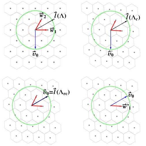
Figure 2: Illustration of Algorithm 1 in two dimensions. Initial optimal lattice (top left) with the basis $\{\vec{w}_{1},\vec{w}_{2}\}$, resolution vector $\vec{v}_{0}$ defining constraint surface and vector $\vec{l}$ is contracted along the vector $\vec{l}$ (top right) and rotated (bottom left) such that for the new lattice $\vec{l}=\vec{v}_{0}$. Final suboptimal lattice has basis $\{\vec{v}_{0},\vec{w}_{1}^{\prime}\}$ (bottom right).

However when the vector $\vec{l}(\Lambda)$ initially lies on the ”constraint surface” depicted by the dashed circle in the Fig. 2 the procedure acts trivially (no contraction only rotation) leaving the final lattice optimal. One often encounters trivial procedures when the vector $\vec{l}(\Lambda)$ is large as compared to the Voronoi cell and moreover in these cases contractions are small. On the other hand the last trivial procedure occurs when the resolution vector and the shortest lattice vector have equal lengths.

One can determine the values of covering radii for which the final lattices are optimal. As an example we find the values of four largest covering radii having this property. To do this we consider the sequence of the shortest vectors of the lattice. In three and four dimensions the first nonzero shortest vectors of $A^{*}_{3}$ and $A^{*}_{4}$ lattices have lengths $2\sqrt{3/5}R(A^{*}_{3})$, $4/\sqrt{5}R(A^{*}_{3})$, $4\sqrt{2/5}R(A^{*}_{3})$, $2\sqrt{1/11}R(A^{*}_{3})$, $\ldots$ and $\sqrt{2}R(A^{*}_{4})$, $\sqrt{3}R(A^{*}_{4})$, $\sqrt{5}R(A^{*}_{4})$, $\sqrt{7}R(A^{*}_{4})$, $\ldots$ respectively. The length of the resolution vector which in dimensionless units has the from $\vec{v}_{0}=(2\pi,0,\ldots)$ is equal to $\sqrt{\tilde{\Gamma}(\vec{v}_{0},\vec{v}_{0})}=\pi/\sqrt{3}$ in both dimensions. This gives the following squares of the largest covering radii for optimal constrained lattices: $R(A^{*}_{3})^{2}$: $5/36\pi^{2}\approx 1.3708$, $5/48\pi^{2}\approx 1.0281$, $5/96\pi^{2}\approx 0.514$, $5/132\pi^{2}\approx 0.3739$, $\ldots$ and $R(A^{*}_{4})^{2}$: $\pi^{2}/6\approx 1.6450$, $\pi^{2}/9\approx 1.0966$, $\pi^{2}/15\approx 0.6580$, $\pi^{2}/21\approx 0.4700$ [points a, b, c, d on Fig.(3)]. For larger values of $R$ thickness of final lattices grows monotonically with covering radius.

These features are seen in the Fig. 3 which shows the results of application of the construction to the model (103) in 3 and 4 dimensions for different covering radii. The resolution vector is $\vec{v}_{0}=(2\pi,0,\ldots)$ and the observation time is 2 years.

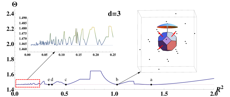
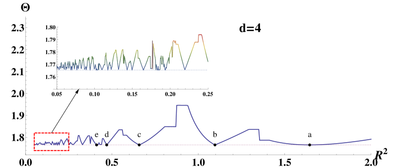
Figure 3: Thickness of the lattices in 3 and 4 dimensions compared to the optimal thickness of $A^{*}_{3}\approx 1.4635$ and $A^{*}_{4}\approx 1.7655$. The upper diagram shows also the optimal lattice with covering radius $R(A^{*}_{3})^{2}=5/48\pi^{2}$. The Voronoi cell, basis vectors, resolution vector and part of the constraint surface are depicted; for this specific value of $R$ the head of the resolution vector lies on the constraint surface.

As for a fixed volume of the parameter space the number of points needed to cover the space with balls of a given radius (i.e. for allowed loss of signal-to-noise ratio) is proportional to the thickness, the diagram demonstrates that the excess of points due to constraints is minor for the wide range of radii which makes the search strategy based on FFT effective.

IV.4 Number of false alarms

In order to estimate the number of false alarms expected in our search we use a general approach consisting of dividing the parameter space into elementary cells defined by the autocorrelation function of the ${\cal F}$-statistic (JK and JKbook Chapter 6.1.3). We use the Taylor expansion of the autocorrelation function around the true values of the parameters $\theta_{k}$ and moreover we use an approximate response of the detector given by the linear model (Eq.  (124) or (125)). In this case the hypervolume of the elementary cell is given by the volume $V_{c}$ of the hyperellipsoid defined as

$$\tilde{\Gamma}_{kl}\Delta\theta_{k}\Delta\theta_{l}\leq 1/2.$$ (90)

Thus $V_{c}$ is given by

$$V_{c}=\frac{(\pi/2)^{m/2}}{\Gamma(m/2+1)\,\sqrt{\det\tilde{\Gamma}}},$$ (91)

where $m$ is the dimension of the parameter space and $\Gamma$ denotes the Gamma function. The determinants of the reduced Fisher matrix in 3 and 4 dimensional cases read

$$\det\tilde{\Gamma_{3}}=\frac{T_{o}^{2}}{48}\frac{\pi^{2}n^{2}-6}{\pi^{2}n^{2}}$$ (92)

$$\det\tilde{\Gamma}=\frac{T_{o}^{6}}{34560}\frac{(\pi^{2}n^{2}-6)(\pi^{4}n^{4}-90)}{\pi^{6}n^{6}},$$ (93)

where it is assumed that the observation time $T_{o}$ is an integer multiple $n$ of years. As for the linear model the reduced Fisher matrix has components independent of the values of the parameters and the number of cells is simply given by

$$N_{c}=\frac{V}{V_{c}},$$ (94)

where $V$ is the hypervolume of the parameter space. We assume that we search a narrow band of bandwidth $\Delta\omega$ with upper frequency $\omega_{\mathrm{max}}$. Then the volume of the parameter space $V_{3}$ when the frequency drift is not included in the search is given by

$$V_{3}=2\Delta\omega\,\pi\,\omega_{\mathrm{max}}^{2}R^{2}$$ (95)

whereas the hypervolume $V_{4}$ when it is included is given by

$$V_{4}=V_{3}\,\Delta\dot{\omega},$$ (96)

where $\Delta\dot{\omega}$ is the range of the frequency drift parameter $\dot{\omega}$. The factor of 2 in Eq. (95) is because we search the space spanned by parameters $\omega$, $\dot{\omega}$, $A$, and $B$ twice - both for positive and negative values of the ecliptic latitude $\beta$.

The expected number of the false alarms $N_{F}$ is given by

$$N_{F}=N_{c}P_{F}({\mathcal{F}}_{o}),$$ (97)

where $P_{F}$ is the probability of false alarm. In the case of linear model $P_{F}$ is the $\chi^{2}$ probability distribution with two degrees of freedom i.e.

$$P_{F}({\mathcal{F}}_{o})=\exp(-{\mathcal{F}}_{o})$$ (98)

IV.5 Computation of the ${\mathcal{F}}$-statistic

The ${\mathcal{F}}$-statistic is computed approximately taking advantage of the speed of the FFT algorithm as described in Section IV.1. The ${\mathcal{F}}$ is calculated on the grid constructed in Section IV.3. For each parameter pair $(A,B)$ the ${\mathcal{F}}$-statistic is computed for both positive and negative value of the ecliptic latitude $\beta_{\rm mid}$ (see Eq. (80)). Approximate calculation of the ${\mathcal{F}}$-statistic on the grid described above is called the coarse search. Using the coarse search we identify signals for which the ${\mathcal{F}}$-statistic crosses a certain threshold. The coarse search is then followed by the second step which we call the fine search. Fine search consists of a search for the maximum of the ${\mathcal{F}}$-statistic around the parameters identified by the coarse search. To find the maximum we use the Nelder-Mead maximization algorithm LRWW98 . In the fine step we use accurate expressions for the ${\mathcal{F}}$-statistic [Eq. (59) or (75)], without approximations described in Section IV.1. As initial values for the Nelder-Mead algorithm we use the parameters obtained in the coarse search. The values of the parameters corresponding to the maximum of ${\mathcal{F}}$-statistic are our final estimates of the parameters of the signal.

V Search strategy

In our entry for challenge $3.1$ we have used the following procedure to extract GW signals from white dwarf/white dwarf binaries in the mock LISA data. We search the band from frequency $f=0.1$ mHz to frequency 12 mHz where $f=\omega/2\pi$. We do not go to higher frequencies because with our search strategy it would involve much more computing time than we could afford. Also above 12 mHz the expected number of white dwarf binaries in our Galaxy is very small. We first divide the data into bands of 0.1 mHz each. To obtain narrowband data in the frequency band $[f_{1}\,\,\,f_{2}]$ we first pass the data through 3rd order Butterworth filter with passband of $[f_{1}-\epsilon\,\,\,f_{2}+\epsilon]$ where we choose the edge parameter $\epsilon$ equal to 0.005 mHz. Then we shift the data to DC by frequency $f_{1}-\epsilon$ and we pass it again through the 3rd order Butterworth filter with passband of $[f_{2}-f_{1}+2\epsilon]$. After each Butterworth filter we downsample the data. This reduces the number of data points by a factor of around 300. Each Butterworth filter is applied twice: forward and backward in time. In this way there is no phase shift of the narrowbanded data with respect to the original one. In the search of each narrow band for signals we neglect the edges of the band of $\epsilon=0.005$ mHz and therefore we only search the band $[f_{1}\,\,\,f_{2}]$. We have included in our search the frequency drift parameter $\dot{\omega}$. Analysis of the accuracy of estimation of $\dot{\omega}$ have shown (see Section VI below) that it is useful to include the $\dot{\omega}$ parameter in the search for frequencies above $3$mHz. We have selected the range of the $\dot{\omega}$ parameter using a fit from the values of the $\dot{\omega}$ parameter in the key of the challenge 3.1 training data set. In each band we search for the signals calculating the ${\cal F}$-statistic over the constrained grid constructed in Section IV.3. This enables application of the FFT algorithm in ${\mathcal{F}}$-statistic computation. We select the strongest signal and to this signal we apply the fine search described in Section IV.5 to estimate its parameters. We use the Nelder-Mead algorithm with the initial values provided by the parameters of the template with the largest value of the ${\cal F}$-statistic over the grid. We reconstruct the signal in the time domain and remove it from the data. We then search for the next strongest signal and so on until the signal-to-noise ratio (SNR) of the detected signal estimated as

$$SNR=\sqrt{2({\mathcal{F}}-2)}$$ (99)

falls below a certain threshold. We have chosen the threshold for the ${\cal F}$-statistic equal to 18. This corresponds to SNR threshold of around 5.7 (see Eq. (99)). The number of signals increases as the signal-to-noise ratio decreases. At a sufficiently low signal-to-noise ratio the signals are so close to each other in the parameter space that they interfere with each other. The ${\mathcal{F}}$-statistic (Eq. 75) that we use in our search was derived under the assumption that there was only one signal present in the data so it can be used to detect multiple signals when they are sufficiently separated in the parameter space so that the ${\mathcal{F}}$-statistic for the multiple signals is a sum of the ${\cal F}$-statistics for individual signals. Thus when there are many signals present we neglect the interference between the signals. Our choice of 18 of the threshold for the ${\cal F}$-statistic was a convenient choice that, as we shall see in the following section, led to a detection and accurate estimation of over $10^{4}$ signals.

In the Figs. 4 and 5 we have presented application of the above strategy to the challenge 3.1 data set in the bandwidth from 5 mHz to 5.1 mHz.

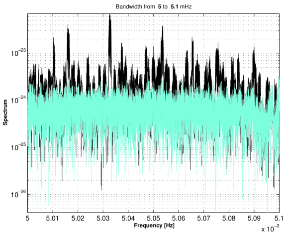
Figure 4: Estimation of the signals from white dwarf binaries in the challenge 3.1 data set for the band from 5 mHz to 5.1 mHz. Black color denotes the original data and the light blue color is the data after signals removed.

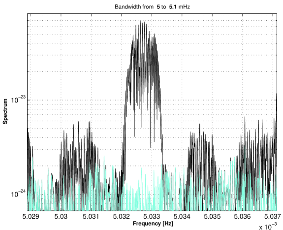
Figure 5: The zoom of the Fig. 4 around the strongest signal identified.

In this bandwidth we have identified 132 signals altogether out of 168 present. The accuracy of estimation of most of the signals is one sigma where sigma is calculated from the Fisher matrix. For several signals the error was very large indicating that either noise mimicked the signal or the residuals of removed signals remained significant. This could happen as a result of interference of the signals.

VI MLDC results

Here we present results of our entry for challenge $3.1$ web:mldc . The challenge $3.1$ consisted of a two-year data set with $15$ s sampling time with signals from around $6\times 10^{7}$ binaries. Our aim was to detect as many as possible from the 40628 brightest binaries present in the data. We have performed a self-evaluation of our search by the following procedure. In our procedure we have used the correlation $C(s_{1},s_{2})$ between the two signals $s_{1}$ and $s_{2}$ defined as

$$C(s_{1},s_{2}):=\frac{{\langle s_{1},s_{2}\rangle}_{\cal S}}{\sqrt{{\langle s_{1},s_{1}\rangle}_{\cal S}}\sqrt{{\langle s_{2},s_{2}\rangle}_{\cal S}}}.$$ (100)

The first step of our self-evaluation consisted of selection of the true detected signals from the set of all submitted data. For a submitted signal $s$ with parameters $\theta_{s}$ we considered set ${\bf B}_{s}$ of all key signals within the frequency bins about $f_{s}$, i.e. signals satisfying

$$|f_{s}-f_{k}|<1/T_{obs}\approx 1.6\times 10^{-8}\mbox{Hz},$$

where parameters $\theta_{k}$ of the key signals were taken from the set of $40628$ bright Galactic binaries web:mldc . Next, each signal $s$ was paired with the key signal $k_{s}$ from ${\bf B}_{s}$ that maximizes the correlation:

$$s\mapsto k_{s}:\;\;\;\;\;\;k_{s}=\arg\max_{k\in{\bf B}_{s}}C\left(s,k\right)\,;$$ (101)

we interpreted $\theta_{s}$ as the parameters estimates of the key signal $k_{s}$. In the case of multiple detection of a key signal $k_{0}$, that is when $k_{s_{1}}=k_{s_{2}}=\ldots=k_{0}$ for different $s_{1}$, $s_{2}$, $\ldots$, as the main signal $s_{k_{0}}$ we singled out the one that maximizes the correlation with $k_{0}$,

$$s_{k_{0}}=\arg{\max_{s:\,k_{s}=k_{0}}}C\left(s,k_{0}\right),$$ (102)

and we rejected the remaining secondary signals.

VI.1 Original results

Our original entry for challenge $3.1$ contained a bug in our data reading procedure. Our analysis for frequencies above $3$mHz was performed on the challenge data set shifted in time by $1440$s. In the original search we have detected 14838 signals altogether and we have estimated their parameters. Results of detection are displayed in Fig. 6 which shows detected (main) signals and the correlations with signals from the key.

Figure 6: Detection and correlations for the blind challenge $3.1$ data set in the original run. The left panel shows number of the signals detected by our search and selected by the procedure described in the text as a function of the frequency. The right panel displays the histogram of the correlation functions (Eq. (100)) between our estimated signals and the ones form the key.

We see that the histogram of the correlations shows an excess of anticorrelations due to the bug in our data reading procedure.

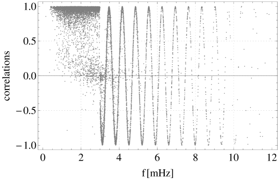
Figure 7: Correlations vs. frequency. The periodic variation of the correlation function was due a time shift in reading of the challenge data set.

Effects of this systematic error can be seen in the Fig. 7 displaying correlations as the function of the frequency. Peculiar oscillations of the correlation with frequency are easily explained by noticing that the phase difference between nearly monochromatic signal and the same signal shifted in time by $t_{0}$ is equal to $2\pi ft_{0}$ and gives periodically changing overlap between the two functions which oscillates with respect to $f$ with ”frequency” $t_{0}$ or by explicitly computing correlation of two monochromatic waves $\cos{[2\pi f(t-t_{0})]}$ and $\cos{(2\pi f)}$. This explains the excess of signals with anticorrelations in Fig. 6.

VI.2 Corrected results

We have corrected the bug in the reading procedure and have made a second run of the challenge $3.1$ data set. Here we present results of this second run. In our search we have detected 17051 signals altogether and we have estimated their parameters.

In the band from 0.1mHz to 3mHz we have made two runs - one with and the other without the $\dot{\omega}$ parameter included. We have used these two runs to investigate at what frequency it is useful to start estimating the frequency drift of the GW signal. In the search including the $\dot{\omega}$ parameter, we have found that we can start estimating it only above frequency of 0.5 mHz because below this frequency the cell of our 4-dimensional grid is bigger than our parameter space. Including the frequency derivative from 0.5mHz we have identified 16785 signals and including $\dot{\omega}$ starting only from 3mHz we have found 17051 signals. We have compared the absolute values of the errors in $\dot{\omega}$ when we include it in the search and when we do not include it. When we do not include it we take as the error the absolute value of the $\dot{\omega}$ parameter from the challenge key signal. We calculate the mean values of the these absolute errors in each band. We find that slightly below the frequency of 3mHz the mean error for the case when we include $\dot{\omega}$ parameter becomes less than when we do not include it. Thus we find that our initial choice of threshold frequency equal to 3 mHz to include the $\dot{\omega}$ is a reasonable one. Therefore, as our final result, we consider the signal found using the search that turns on the frequency derivative at 3mHz frequency. We have also estimated the expected number of false alarms using the formula (97) in Section IV.4. We find that for low frequencies where we detect most of our signals the number of false alarms is negligible. The number of false alarms increases quadratically with frequency and linearly with the range of $\dot{\omega}$ parameter. The expected number of false alarms exceeds one only at the frequency $f=8$ mHz.

In Fig. 8 we present the number of signals detected against all the challenge $3.1$ signals and the correlations of the estimated signals with the key signals in the second run.

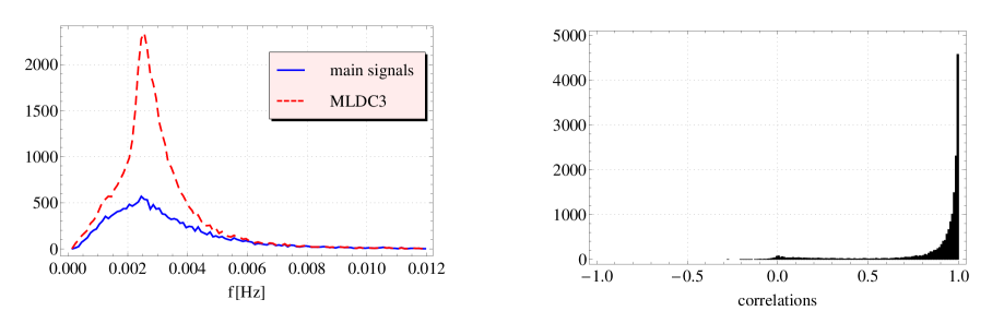
Figure 8: Detection and correlations for the blind challenge $3.1$ data set in the second run.

We see that there is still an excess of correlations with correlation parameter around zero. We have investigated the number of correlations as a function of signal-to-noise ratio (see Fig. 9).

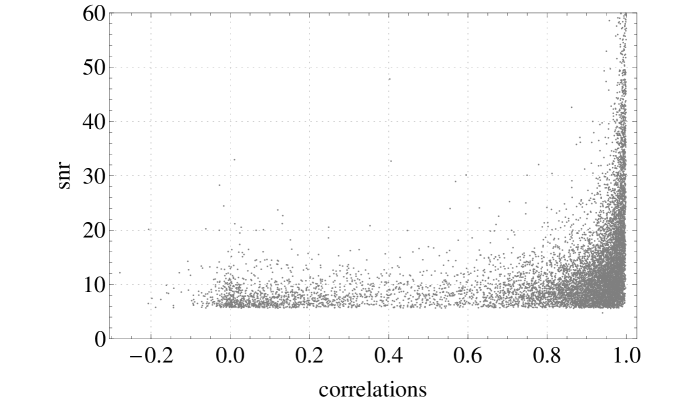
Figure 9: Number of correlations of estimated signals with key signals as a function of the signal-to-noise ratio for signals with frequency below 3 mHz.

We find that the excess of low correlations originates from frequencies below 3 mHz. Moreover for SNR $>10$ the number of small correlations considerably decreases. The number of selected signals after we discarded signals below SNR $=10$ and for frequency less than 3 mHz is 12805. We quote this number as the number of signals which we detect and accurately estimate the parameters. We need to refine our data analysis methods in order to extract reliable estimates of the parameters for the signals of SNR less than 10 and frequency less than 3 mHz.

The excess of zero correlation signals arises either because for some low signal-to-noise ratio the parameter estimation was not accurate or/and because at low signal-to-noise ratio there are much more signals that interfere causing biases in the parameter estimators. Fig. 10 demonstrates the results of the parameter estimations for our search of challenge 3.1 data set. Errors are defined as differences between the key and the recovered signal parameters, $\Delta\theta:=\theta_{key}-\theta_{rec}$. Histograms in Fig. 11 show the parameter estimation errors divided by the standard deviations $\sigma_{\theta_{key}}$ obtained from the Fisher matrix for the key signals.

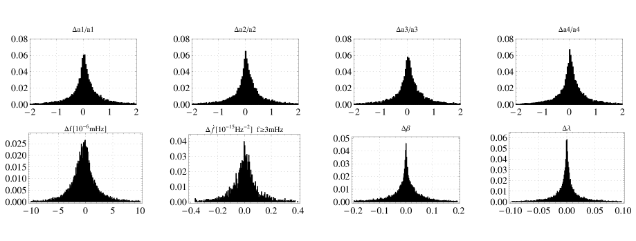
Figure 10: Errors of the parameters of the signals detected and verified in our search of the challenge $3.1$ data set.

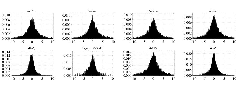
Figure 11: Errors of the estimation of parameters as in Fig. 10 but normalized by the variances obtained from the inverse of the Fisher information matrix.

In Fig. 12 we have presented the power spectrum of the challenge 3.1 data against the power spectrum of the data after the detected signals were removed. We plot two power spectra: one when all the signals identified are removed and the other one when only the ones selected by our procedure are removed form the challenge data set. We notice two effects. One is that periodically our identification procedure gets worse. This because we were not estimating parameters of the signal very well at the edges of the narrow bands. We have found that this is because our narrowband filtering procedure was not perfect. The other effect is that when we remove all identified signals (lower signal on the Fig. 12) we are doing a much better job then when we remove only signals identified as true signals by our procedure (middle signal on the Fig. 12). Thus we fit quite a large number of signals well but with wrong parameters.

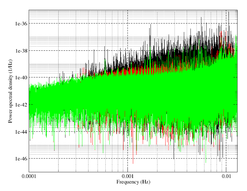
Figure 12: Amplitude square of the Fourier transformed data. Upper signal is original challenge data (A-channel, includes full Galaxy and instrumental noise), middle is the data with selected removed signals, and lower is the data with all identified signals removed.

In Fig. 13 we have compared smoothed spectrum of the challenge 3.1 data set with that of data with identified signals removed and we have compared them with spectrum of the LISA detector instrumental noise.

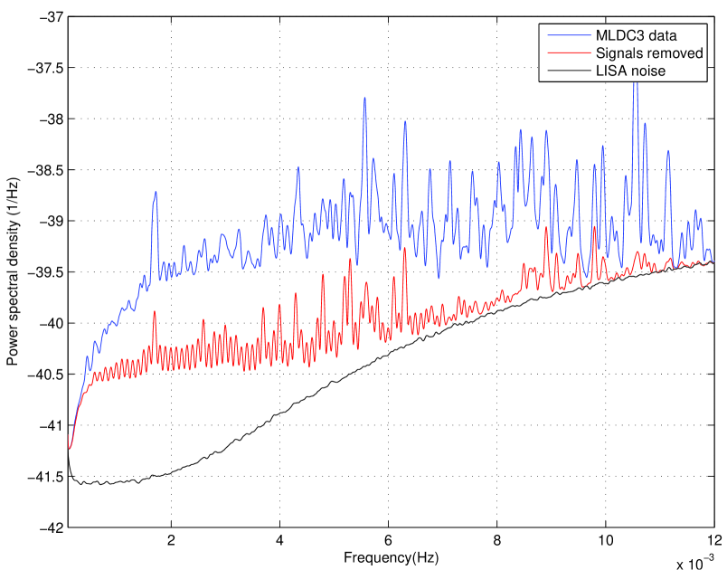
Figure 13: Power spectral density. Upper signal is the original challenge data, middle is reduced data (after removing all found signals), and lower is the instrumental noise.

From this figure we conclude that above frequency of $6$ mHz we resolve all the white-dwarf binary systems well.

VII Conclusion

From the analysis of our challenge $3.1$ results we see that in order to increase substantially the number of signals with good parameter estimation we need to assume in deriving our filters that there are more than one signal present in the data. However even with the current procedure that estimates signals one by one we can still make the following improvements.

1. Improve the splitting of the time series into narrow bands.

2. Lower the threshold for detection.

3. For high frequencies bands where signals are well separated identify all the signals at one scan of the parameter space instead extracting only one and scanning the whole parameter space again to go to the next.

Appendix A Linear model

In this appendix we consider the linear model, an approximation of the full gravitational wave signal introduced in order to construct a metric and a grid on the intrinsic parameter space. It has the form:

$$s(t)=A_{0}\cos{(\omega t+\frac{1}{2}\dot{\omega}t^{2}+A\cos{\Omega t}+B\sin{\Omega t}+\phi_{0})},$$ (103)

with constant amplitude $A_{0}$, constant phase $\phi_{0}$ and two parameters $A$, $B$ (related to $\omega$, $\beta$ and $\lambda$).

Following the general case (1) we rewrite the signal (103) in the form

$$s(t)=A_{1}X_{1}(t)+A_{2}X_{2}(t),$$ (104)

where

$$X_{1}=\cos{(\omega t+\frac{1}{2}\dot{\omega}t^{2}+A\cos{\Omega t}+B\sin{\Omega t})},$$

$$X_{2}=\sin{(\omega t+\frac{1}{2}\dot{\omega}t^{2}+A\cos{\Omega t}+B\sin{\Omega t})}$$

and where we have introduced the extrinsic amplitudes $A_{1}=h_{0}\cos{\phi_{0}}$ and $A_{2}=-h_{0}\sin{\phi_{0}}$.

The Fisher matrix,

$$\Gamma_{ij}=\frac{2T_{o}}{S(\omega_{o})}{\langle\partial_{i}s\;\partial_{j}s\rangle},$$ (105)

for the linear model (104) with respect to the parameters $(A_{1},A_{2},\omega,\dot{\omega},A,B)$ takes the form

$$\Gamma=\left(\begin{array}[]{cc}{\bf G}_{1}&{\bf G}_{2}\\ {\bf G}_{2}{}^{T}&{\bf G}_{3}\end{array}\right),$$ (106)

where

$${\bf G}_{1} = \rho^{2}\left(\begin{array}[]{cc}\frac{1}{A_{1}{}^{2}+A_{2}{}^{2}}&0\\ 0&\frac{1}{A_{1}{}^{2}+A_{2}{}^{2}}\end{array}\right)$$ (109)

$${\bf G}_{2} = \rho^{2}\left(\begin{array}[]{cccc}\frac{T_{o}{}A_{2}}{2(A_{1}{}^{2}+A_{2}{}^{2})}&\frac{T_{o}{}^{2}A_{2}}{6(A_{1}{}^{2}+A_{2}{}^{2})}&0&0\\ -\frac{T_{o}{}A_{1}}{2(A_{1}{}^{2}+A_{2}{}^{2})}&-\frac{T_{o}{}^{2}A_{1}}{6(A_{1}{}^{2}+A_{2}{}^{2})}&0&0\\ \end{array}\right)$$ (112)

$${\bf G}_{3} = \rho^{2}\left(\begin{array}[]{cccc}\frac{T_{o}{}^{2}}{3}&\frac{T_{o}{}^{3}}{8}&0&-\frac{1}{\Omega}\\ \frac{T_{o}{}^{3}}{8}&\frac{T_{o}{}^{4}}{20}&\frac{1}{\Omega^{2}}&-\frac{T_{o}}{2\Omega}\\ 0&\frac{1}{\Omega^{2}}&\frac{1}{2}&0\\ -\frac{1}{\Omega}&-\frac{T_{o}}{2\Omega}&0&\frac{1}{2}\end{array}\right),$$ (117)

and where the optimal signal-to-noise ratio,

$$\rho^{2}=\frac{2T_{o}}{S(\omega_{o})}{\langle s^{2}\rangle},$$ (118)

is given by $\rho^{2}=\frac{T_{o}(A_{1}{}^{2}+A_{2}{}^{2})}{S(\omega_{o})}$ and the observation time $T_{o}$ is assumed to be an integer $n$ of years. In the derivation of Eqs. (109) - (118) we have used the following approximations

$${\langle X_{1}{}^{2}\rangle}\simeq{\langle X_{2}{}^{2}\rangle}\simeq\frac{1}{2},\;\;\;\;\;\;{\langle X_{1}\,X_{2}\rangle}\simeq 0$$ (119)

corresponding to approximations (43)-(51) for the case of the full signal.

The reduced Fisher matrix obtained from the full Fisher matrix $\Gamma$ by projecting $\Gamma$ on the intrinsic parameters space and normalizing it is explicitly given by (JK )

$$\tilde{\Gamma}=\frac{1}{\rho^{2}}\left({\bf G}_{3}-{\bf G}_{2}{}^{T}\,{\bf G}_{1}{}^{-1}\,{\bf G}_{2}\right)$$ (120)

The coefficients of the reduced Fisher matrix $\tilde{\Gamma}$ of the linear model (104) in the dimensionless units with $T_{o}=1$ are given by

$$\tilde{\Gamma}=\left(\begin{array}[]{cccc}\frac{1}{12}&\frac{1}{24}&0&-\frac{1}{2\pi n}\\ \frac{1}{24}&\frac{1}{45}&\frac{1}{4\pi^{2}n^{2}}&-\frac{1}{4\pi n}\\ 0&\frac{1}{4\pi^{2}n^{2}}&\frac{1}{2}&0\\ -\frac{1}{2\pi n}&-\frac{1}{4\pi n}&0&\frac{1}{2}\\ \end{array}\right).$$ (121)

For a network of detectors ${\bf s}=(s_{A},s_{E},s_{T})$ with uncorrelated noises the Fisher matrix and the optimal signal-to-noise ratio can be written in terms of the noise-weighted averaging operator and vectorial response [see Sect.(III)]:

$$\Gamma_{opt\,ij}=\frac{2T_{o}}{{\cal S}(\omega_{o})}{\langle\partial_{i}{\bf s}\,\partial_{j}{\bf s}\rangle}_{\cal S},$$ (122)

$$\rho_{opt}{}^{2}=\frac{2T_{o}}{{\cal S}(\omega_{o})}{\langle{\bf s}^{2}\rangle}_{\cal S}.$$ (123)

In the case of network of LISA detectors the optimal responses $A$, $E$, and $T$ can be approximated by the linear model of the form

$$s_{I}(t)=c_{I}h_{0}\cos{(\omega t+\frac{1}{2}\dot{\omega}t^{2}+A\cos{\Omega t}+B\sin{\Omega t}+\phi_{0}+d_{I})},\;\;\;\;\;\;\;\;I=A,E,T,$$ (124)

where constants $c_{I}$ and $d_{I}$ have been introduced in order to take into account different amplitude and phase modulations for each observable. The reduced Fisher matrix for network turns out to be exactly the same as the reduced matrix for a single response. This is the special case of the general property discovered by R. Prix (Prix , Ch. IIIC) that grid resolution in the parameter space is independent of the number of detectors.

For low frequencies the frequency derivative $\dot{\omega}$ is small and there is no need to include this parameter in the search. Then the linear model simplifies to

$$s_{3I}(t)=c_{I}h_{0}\cos{(\omega t+A\cos{\Omega t}+B\sin{\Omega t}+\phi_{0}+d_{I})},\;\;\;\;\;\;\;\;I=A,E,T$$ (125)

and the corresponding reduced Fisher matrix $\tilde{\Gamma}_{3}$ reads

$$\tilde{\Gamma}_{3}=\left(\begin{array}[]{cccc}\frac{1}{12}&0&-\frac{1}{2\pi n}\\ 0&\frac{1}{2}&0\\ -\frac{1}{2\pi n}&0&\frac{1}{2}\\ \end{array}\right).$$ (126)

References

References

- (1) G. Nelemans et al., gr-qc/0902.2923.
- (2) J. A. Edlund, M. Tinto, A. Królak, G. Nelemans, Phys. Rev. D 71, 122003 (2005).
- (3) J. A. Edlund et al., Class. Quantum Grav. 22, S913-S926 (2005).
- (4) G. Nelemans, Class. Quantum Grav. 26, 094030 (2009) and references therein.
- (5) A. Stroeer and A. Vecchio, Class. Quantum Grav. 23, S809-S818 (2006).
- (6) S. Babak et al., Class. Quantum Grav. 25:114037 (2008).
- (7) MLDC homepage, http://astrogravs.nasa.gov/docs/mldc/.
- (8) K. A. Arnaud et al., AIP Conf. Proc. 873, 619 (2006).
- (9) K. A. Arnaud et al., Class. Quantum Grav. 24, S529-S539 (2007).
- (10) K. A. Arnaud et al., Class. Quantum Grav. 24, S551-S564 (2007).
- (11) G. Nelemans, L. R. Yungelson, and S. F. Portegies Zwart, Astron. Astrophys. 375, 890 (2001).
- (12) G. Nelemans, L. R. Yungelson and S. F. Portegies Zwart, Mon. Not. Roy. Astron. Soc. 349 (2004).
- (13) B. Willems, V. Kalogera, A. Vecchio, N. Ivanova, F. A. Rasio, J. M. Fregeau, K. Belczynski, Astrophys. J. 665, L59 (2007).
- (14) M. Benacquista, S. Portegies Zwart, F. Rasio, Class. Quantum Grav. 18, 4025 (2001).
- (15) J. Crowder, N. J. Cornish and J. L. Reddinger, Phys. Rev. D 73, 063011 (2006).
- (16) J. Crowder, Class. Quantum Grav. 24, S575- S586. (2007).
- (17) M. Trias, A. Vecchio and J. Veitch, Class. Quantum Grav. 26, 204024 (2009); gr-qc/0904.2207.
- (18) J. T. Whelan, R. Prix and D. Khurana, Class. Quantum Grav. 27, 055010. (2007).
- (19) M. Tinto, S. V. Dhurandhar, Living Rev. Relativity 8, (2005) 4: http://www.livingreviews.org/lrr-2005-4.
- (20) S. D. Mohanty and R. K. Nayak, Phys. Rev. D 73, 083006 (2006).
- (21) J. W. Armstrong, F. B. Estabrook, and M. Tinto, Astrophys. J. 527, 814 (1999).
- (22) N. J. Cornish and L. J. Rubbo, Phys. Rev. D 67, 022001 (2003).
- (23) A. Królak, M. Tinto, and M. Vallisneri, Phys. Rev. D 70, 022003 (2004); 76 069901(E) (2007).
- (24) M. Vallisneri, Phys. Rev. D 71, 022001 (2005).
- (25) K. A. Arnaud et al., AIP Conf. Proc. 873, 625 (2006).
- (26) A. D. Whalen, Detection of Signals in Noise, (Academic Press, New York, 1971).
- (27) T. A. Prince, M. Tinto, S.L. Larson, and J.W. Armstrong, Phys. Rev. D 66, 122002 (2002).
- (28) Note that the optimal combinations are not unique.
- (29) P. Astone, K. M. Borkowski, P. Jaranowski and A. Królak, Phys. Rev. D 65, 042003 (2002).
- (30) R. Balasubramanian, B. S. Sathyaprakash and S. V. Dhurandhar, Phys. Rev. D 53, 3033 (1996).
- (31) B. J. Owen, Phys. Rev. D 53, 6749 (1996).
- (32) A. Błaut, A. Królak and S. Babak, Class. Quantum Grav 26, 204023 (2009).
- (33) P. Jaranowski, A. Królak ”Gravitational-wave data analysis. Formalism and simple applications: the Gaussian case”, Living Rev. Relativity 8, (2005)3: http://www.livingreviews.org/lrr-2005-3.
- (34) Reinhard Prix, Phys. Rev. D 75, 023004 (2007).
- (35) J.H. Conway and N.J.A. Sloane, Sphere Packings, Lattices and Groups (Springer-Verlag, New York, 1993)
- (36) P. Jaranowski and A. Królak, Analysis of Gravitational-Wave Data (Cambridge University Press, Cambridge, 2009).
- (37) J. C. Lagarias, J. A. Reeds, M. H. Wright, and P. E. Wright, SIAM J. Optim. 9, 112 (1998).