Quantifying spin Hall angles from spin pumping: Experiments and Theory
Abstract
Spin Hall effects intermix spin and charge currents even in nonmagnetic materials and, therefore, ultimately may allow the use of spin transport without the need for ferromagnets. We show how spin Hall effects can be quantified by integrating Ni80Fenormal metal (N) bilayers into a coplanar waveguide. A dc spin current in N can be generated by spin pumping in a controllable way by ferromagnetic resonance. The transverse dc voltage detected along the Ni80FeN has contributions from both the anisotropic magnetoresistance (AMR) and the spin Hall effect, which can be distinguished by their symmetries. We developed a theory that accounts for both. In this way, we determine the spin Hall angle quantitatively for Pt, Au and Mo. This approach can readily be adapted to any conducting material with even very small spin Hall angles.
pacs:
72.25.Rb, 75.47.-m, 76.50.+gThe spin-orbit interaction gives rise to spin-dependent scattering that can couple charge and spin currents in conducting materials. Resultant spin Hall effects Dyakonov and Perel (1971); Hirsch (1999); Zhang (2000) may therefore display spin-dependent transport even in materials and device structures that do not contain ferromagnetic materials. The effectiveness of this spin-charge conversion can be quantified by the material-specific spin Hall angle , which is given by the ratio of spin Hall and charge conductivities Dyakonov and Khaetskii (2008) and can be quantified by magnetotransport measurements Fert et al. (1981); Valenzuela and Tinkham (2006); Kimura et al. (2007); Seki et al. (2008); Morota et al. (2009). However, values reported in the literature vary over several orders of magnitude even for nominally identical materials (i.e., Au: Mihajlović et al. (in press) and Seki et al. (2008), and Pt: Kimura et al. (2007) and Ando et al. (2008a)). In order to better understand spin-dependent scattering and its potential use for spin-transport applications it is therefore highly desirable to find a robust method to quantify . Here we demonstrate an approach whose sensitivity can be adjusted to measure even very small values of .
Previous work on ferromagnetic resonance (FMR) in magnetic multilayers has shown that spin pumping can create pure spin currents in normal metals (N) Heinrich et al. (2003); Woltersdorf et al. (2007); Mosendz et al. (2009). Upon excitation of FMR, the time-varying magnetization inside the ferromagnet (F) generates an instantaneous spin current at the FN interface given by Tserkovnyak et al. (2002a); Tserkovnyak et al. (2005):
| (1) |
where is the unit vector of the magnetization, is the unit vector of the spin current polarization, and is the real part of the spin mixing conductance. Under a simple precession endnote the spin pumping induces a net dc spin current and by time-averaging Eq. (1) we get:
| (2) |
where is the driving frequency and is the cone angle of the precession of . This spin current decays due to spin relaxation and diffusion in N, such that the spin current at distance from the interface is:
| (3) |
where is the materials specific spin diffusion length and is the thickness of the N layer.
The spin current gives rise to a transverse charge current due to the inverse spin Hall effect (ISHE). It has already been demonstrated that this transverse charge current can be observed as a dc voltage Saitoh et al. (2006); Ando et al. (2008b); Azevedo et al. (2005). Here we show how an approach based on spin pumping can be applied to various FN combinations. We identify two contributions to the dc voltage that stem from anisotropic magnetoresistance (AMR) and spin Hall effect, respectively, and can be distinguished by their symmetries. Furthermore, we present a self-consistent theory that enables quantification of the spin Hall angle with high accuracy.
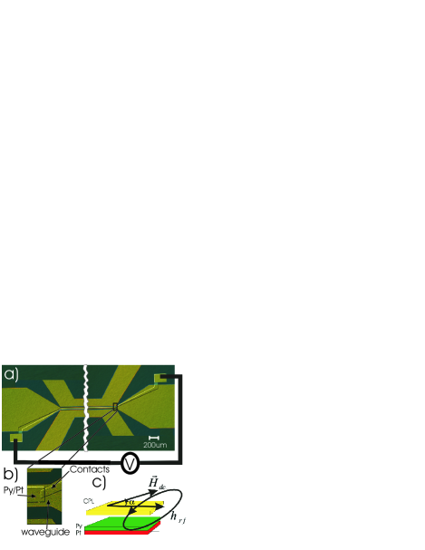
We integrated FN bilayers into coplanar waveguides with additional leads for measuring a dc voltage along the sample. This is shown in Fig. 1 for a Ni80Fe20 (Py)Pt bilayer, with lateral dimensions of 2.92 mm 20 m and 15-nm thick individual layers. The bilayer was prepared by optical lithography, sputter deposition, and lift-off on a GaAs substrate. Subsequently we prepared Ag contacts for the voltage measurements, covered the whole structure with 100-nm thick MgO (for dc insulation between bilayer and waveguide), and defined a 30-m wide and 200-nm thick Au coplanar waveguide on top of the bilayer. Similar samples were prepared with 60-nm thick Au and Mo layers replacing Pt.
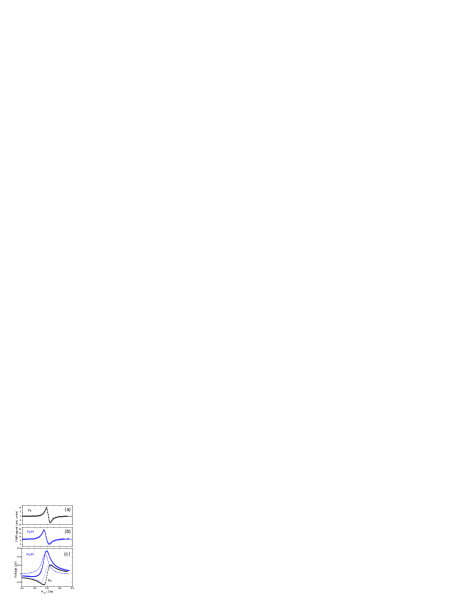
The FMR was excited by a 4-GHz, 100-mW rf excitation, while applying a dc magnetic field at with respect to the waveguide [see Fig. 1(c)]. The FMR signal was determined from the impedance of the waveguide Mosendz et al. (2008); simultaneously the dc voltage was measured as a function of . Figure 2 shows this for a PyPt bilayer and a Py single layer, where both FMR peak positions are similar and consistent with the Kittel formula:
| (4) |
where is the gyromagnetic ratio, is the electron g-factor and G is the saturation magnetization for Py. The FMR linewidths (HWHM) extracted from fits to Lorentzian absorption functions are Oe for PyPt and Oe for Py. The difference in FMR linewidth can be attributed to the loss of spin momentum in Py due to relaxation of the spin accumulation in Pt. This permits the determination of the additional interface damping due to spin pumping Urban et al. (2001), which in turn provides the interfacial spin mixing conductance as:
| (5) |
where is the Py layer thickness and is the Bohr magneton (spin backflow being disregarded since Pt is an efficient spin sink). The calculated value for m-2 is somewhat smaller than the previously reported m-2 Mizukami et al. (2001); Tserkovnyak et al. (2002b), but Cao et al. Cao et al. (2009) showed that for high power rf excitation, the spin mixing conductance is reduced due to the loss of coherent spin precession in the ferromagnet.
Figure 2(c) shows the dc voltage measured along the samples. For the PyPt sample we observe a resonant increase in the dc voltage along the sample at the FMR position. However the lineshape is complicated: below the resonance field the voltage is negative, it changes sign just before the FMR resonance field, and has a positive tail in the high field region. In contrast, the single layer Py sample, which is not affected by spin pumping, shows a voltage signal that is purely antisymmetric with respect to the FMR position. The voltage due to ISHE depends only on the cone angle of the magnetization precession [see Eq. (2)] and thus must be symmetric with respect to the FMR resonance position. This means that the voltage measured in the PyPt sample has two contributions: (i) a symmetric signal due to ISHE and (ii) an antisymmetric signal of the same origin as in the Py control sample.
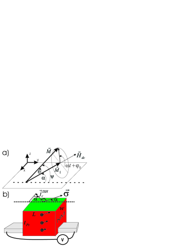
The antisymmetric voltages observed in both Py and PyPt originate from anisotropic magnetoresistance (AMR). Although the MgO provides dc insulation between the sample and the waveguide, there is strong capacitive coupling, and thus part of the rf driving current flows through the sample. This rf current in the sample flows along the waveguide direction and its magnitude can be estimated from the ratio between the waveguide resistance and the sample resistance : . The precessing magnetization in the Py [see Fig. 3(a)] results in a time-dependent due to AMR given by , where is the sample resistance with the magnetization along the waveguide axis and is the angle between the instantaneous magnetization and the waveguide axis [see Fig. 3(a)] Costache et al. (2006). Since the AMR contribution to the resistance oscillates at the same frequency as the rf current, a homodyne dc voltage develops and is given by:
| (6) |
where is the phase angle between magnetization precession and driving rf field and the relation between , and is illustrated in Fig. 3(a). The phase angle is zero well below the FMR resonance, at the peak, and far above the resonance Guan et al. (2006). Thus changes sign upon going through the resonance and this gives rise to an antisymmetric as observed in both Py and PyPt samples. Following Guan et al. Guan et al. (2006) we calculate the cone angle and as a function of the applied field , FMR resonance field , FMR linewidth and rf driving field :
| (7) |
| (8) |
Using Eqs. (6–8) and taking a measured 0.95% value for fits the Py data [see Fig. 2(b)] with only one adjustable parameter Oe.
In order to understand the PyPt voltage data we have to include an additional contribution due to ISHE. In an open circuit an electric field is generated leading to a total current density with where is the N conductivity. When the wire is much longer than thick, the electric field is constant in the wire and the component of the electric field along the measurement direction is:
| (9) |
Using Eq. 9 we calculate the voltage due to ISHE generated along the sample with length :
| (10) |
Note that this voltage is proportional to and thus measurements of small can be achieved by increasing the sample dimension. We used Eqs. (10) and (6) to fit the voltage measured for the PyPt sample, see solid line in Fig. 2(c). The dashed and dotted lines in Fig. 2(c) are the AMR and ISHE contributions, respectively. By using a literature value for Pt of nm Kurt et al. (2002), the only remaining adjustable parameters are the rf driving field Oe and the spin Hall angle . Note that through the cone angle , enters both the AMR and ISHE contributions; this puts an additional constraint on this parameter, and, in fact, as seen from the fit to the control Py sample, it is already determined by the negative and positive tails of the AMR part.
| Normal metal | (nm) | ||
|---|---|---|---|
| Pt | 102 | (2.420.19) | 0.00670.0006 |
| Au | 353 | (2.520.13) | 0.00160.0003 |
| Mo | 353 | (4.660.23) | -0.000230.00005 |
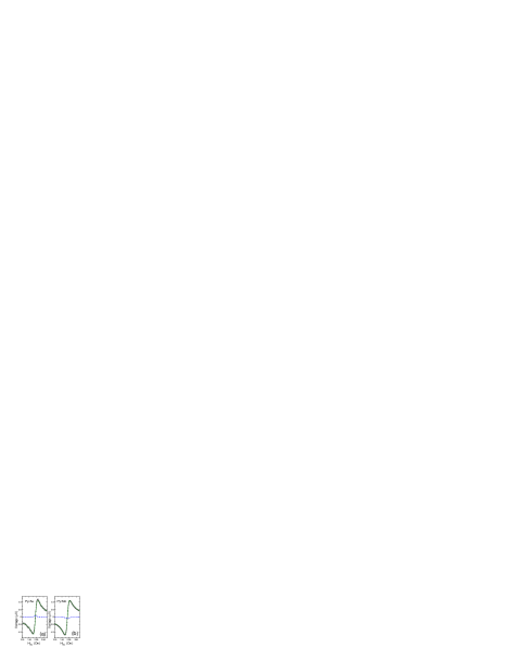
This technique can be readily applied to determine in any conductor. In Fig. 4 we show voltages measured for PyAu and PyMo. The spin Hall contributions in Au and Mo are smaller than in Pt, and note that for Mo the spin Hall contribution changes its sign. Fitting of the data enabled us to extract the values of for Au and Mo, see Table 1. Note that the determination of requires and as an input parameters. was measured using four-probe measurements for all samples. Reported values for vary considerably. We choose a conservatively low literature value for Pt from Ref. Kurt et al., 2002 and Au from Ref. Mosendz et al., 2009, and for Mo we assumed that is comparable to Au. Even though this latter assumption may not necessarily hold, the sign change is consistent with earlier measurements Morota et al. (2009). Furthermore, our observed values for are in good agreement with values reported by Otani et al. Vila et al. (2007); Morota et al. (2009) from measurements in lateral spin valves, but conflict with more optimistic values reported by other groups Seki et al. (2008); Ando et al. (2008a). We note that in lateral spin valves it is important to also understand the charge current contribution in order to rule out additional non-local voltage contributions Mihajlović et al. (in press). In contrast, in our approach the spin pumping creates a uniform, macroscopic and well-defined spin current across the whole sample, and the voltage signal from spin Hall effects can readily be increased through use of longer samples, since . Furthermore, using an integrated coplanar waveguide architecture provides control over parameters, such as the rf driving field distribution. This enables us to carry out a quantitative analysis of the data, in contrast to the more qualitative description of the ISHE in Refs. Saitoh et al., 2006 and Ando et al., 2008b.
In conclusion, we performed FMR with simultaneous transverse voltage measurements in ferromagnetic/normal metal bilayers. From this we accurately determine the spin Hall angle for Pt, Au and Mo by fitting the experimental data to a theory, which accounts for both the anistropic magnetoresistance and inverse spin Hall effect contributions. The combination of spin pumping and spin Hall effects provides a valuable technique for measuring spin Hall angle in many different materials.
We would like to thank R. Winkler, G. Mihajlović and M. Dyakonov for valuable discussions. This work was supported by U.S. DOE-BES under Contract No. DE-AC02-06CH11357.
References
- Dyakonov and Perel (1971) M. Dyakonov and V. Perel, Sov. Phys. JETP Lett. 13, 467 (1971).
- Hirsch (1999) J. Hirsch, Phys. Rev. Lett. 83, 1834 (1999).
- Zhang (2000) S. Zhang, Phys. Rev. Lett. 85, 393 (2000).
- Dyakonov and Khaetskii (2008) M. I. Dyakonov and A. V. Khaetskii, in Spin Physics in Semiconductors, edited by M. I. Dyakonov (Springer, 2008), vol. 157 of Springer Series in Solid-State Sciences, chap. 8, p. 212.
- Fert et al. (1981) A. Fert, A. Friederich, and A. Hamzic, J. Magn. Magn. Mater. 24, 231 (1981).
- Valenzuela and Tinkham (2006) S. O. Valenzuela and M. Tinkham, Nature 442, 176 (2006).
- Kimura et al. (2007) T. Kimura, Y. Otani, T. Sato, S. Takahashi, and S. Maekawa, Phys. Rev. Lett. 98, 156601 (2007).
- Seki et al. (2008) T. Seki, Y. Hasegawa, S. Mitani, S. Takaashi, H. Imamura, S. Maekawa, J. Nitta, and K. Takanashi, Nature Mater. 7, 125 (2008).
- Morota et al. (2009) M. Morota, K. Ohnishi, T. Kimura, and Y. Otani, J. Appl. Phys. 105, 07C712 (2009).
- Mihajlović et al. (in press) G. Mihajlović, J. E. Pearson, M. A. Garcia, S. D. Bader, and A. Hoffmann, Phys. Rev. Lett. 103, 166601 (2009).
- Ando et al. (2008a) K. Ando, S. Takahashi, K. Harii, K. Sasage, J. Ieda, S. Maekawa, and E. Saitoh, Phys. Rev. Lett. 101, 036601 (2008a).
- Heinrich et al. (2003) B. Heinrich, Y. Tserkovnyak, G. Woltersdorf, A. Brataas, R. Urban, and G. E. W. Bauer, Phys. Rev. Lett. 90, 187601 (2003).
- Woltersdorf et al. (2007) G. Woltersdorf, O. Mosendz, B. Heinrich, and C. H. Back, Phys. Rev. Lett. 99, 246603 (2007).
- Mosendz et al. (2009) O. Mosendz, G. Woltersdorf, B. Kardasz, B. Heinrich, and C. H. Back, Phys. Rev. B 79, 224412 (2009).
- Tserkovnyak et al. (2002a) Y. Tserkovnyak, A. Brataas, and G. E. W. Bauer, Phys. Rev. Lett. 88, 117601 (2002a).
- Tserkovnyak et al. (2005) Y. Tserkovnyak, A. Brataas, G. E. W. Bauer, and B. I. Halperin, Review of Modern Physics 77, 1375 (2005).
- (17) circular precession was assumed for simplicity, realistic elliptical precession trajectory will result in a quantitative, but not qualitative modification to the model.
- Saitoh et al. (2006) E. Saitoh, M. Ueda, H. Miyajima, and G. Tatara, Appl. Phys. Lett 88, 182509 (2006).
- Ando et al. (2008b) K. Ando, Y. Kajiwara, S. Takahashi, S. Maekawa, K. Takemoto, M. Takatsu, and E. Saitoh, Phys. Rev. B 78, 014413 (2008b).
- Azevedo et al. (2005) A. Azevedo, L. H. V. Leao, R. L. Rodriguez-Suarez, A. B. Oliveira, and S. M. Rezende, J. Appl. Phys. 97, 10C715 (2005).
- Mosendz et al. (2008) O. Mosendz, B. Kardasz, and B. Heinrich, J. Appl. Phys. 103, 07B505 (2008).
- Urban et al. (2001) R. Urban, G. Woltersdorf, and B. Heinrich, Phys. Rev. Lett. 87, 217204 (2001).
- Mizukami et al. (2001) S. Mizukami, Y. Ando, and T. Miyazaki, J. Mag. Mag. Mat. 226, 1640 (2001).
- Tserkovnyak et al. (2002b) Y. Tserkovnyak, A. Brataas, and G. E. W. Bauer, Phys. Rev. B 66, 224403 (2002b).
- Cao et al. (2009) R. Cao, X. Fan, T. Moriyama, and J. Xiao, J. Appl. Phys. 105, 07C705 (2009).
- Costache et al. (2006) M. Costache, S. Watts, M. Sladkov, C. van der Wal, and B. van Wees, Appl. Phys. Lett 89, 232115 (2006).
- Guan et al. (2006) Y. Guan, W. E. Bailey, E. Vescovo, C. C. Kao, and D. A. Arena, J. Magn. Magn. Mat. 312, 374 (2006).
- Kurt et al. (2002) H. Kurt, R. Loloee, K. Eid, J. W. P. Pratt, and J. Bass, Appl. Phys. Lett. 81, 4787 (2002).
- Vila et al. (2007) L. Vila, T. Kimura, and Y. Otani, Phys. Rev. Lett. 99, 226604 (2007).