Collective versus Single–Particle Motion in Quantum Many–Body Systems from the Perspective of an Integrable Model

Abstract

We study the emergence of collective dynamics in the integrable Hamiltonian system of two finite ensembles of coupled harmonic oscillators. After identification of a collective degree of freedom, the Hamiltonian is mapped onto a model of Caldeira-Leggett type, where the collective coordinate is coupled to an internal bath of phonons. In contrast to the usual Caldeira-Leggett model, the bath in the present case is part of the system. We derive an equation of motion for the collective coordinate which takes the form of a damped harmonic oscillator. We show that the distribution of quantum transition strengths induced by the collective mode is determined by its classical dynamics.

1 Introduction

Many-body systems show incoherent, single-particle-motion, as well as coherent collective motion. Historically this phenomenon received much attention in nuclear physics where there is a wealth of data providing information on the coexistence of collective excitations, such as the Giant Dipole Resonance (GDR), and single particle excitations [1]. There is also strong experimental [2] and theoretical [3] evidence that similar effects occur in fermionic systems different from atomic nuclei. Other examples for collective motion are vortex-generating rotations and oscillations in Bose-Einstein condensates [4, 5, 6]. Furthermore collective behavior can also be present in confined systems such as quantum dots [7, 8].

Coherent, collective motion emerges out of incoherent, single-particle motion whenever favored by energy conditions. Statistical analysis of spectra in nuclei indicates that chaotic fluctuations are due to single-particle motion, while collective motion is predominantly regular, for a review see Ref. [9] and more recent results in Refs [10, 11]. This generic occurrence and the coexistence of the two forms of motion pose a fundamental challenge. Strictly speaking, in a generic many-body system there is not an a priori separation of the collective motion from the single-particle dynamics. Taking the three-dimensional Boltzmann gas with hard-wall interactions as an example, one observes that the dynamics in the phase space of the system is completely chaotic [12]. Still, we know that the system exhibits regular collective motion in the form of sound waves. The deep and fascinating question in this context is therefore to understand from first principles how the regular motion emerges out of the full phase space chaos [13].

Whenever collective dynamics arises on the classical level one might expect on the basis of quantum-classical correspondence that this phenomena should be reflected in the spectral properties of the corresponding quantum many-body Hamiltonian. One way to probe the existence of collective excitations is to couple the system to a weak external periodic potential $V(X)\exp(i\omega t)$ depending on a collective mode $X$. The presence of a collective excitation can then be usually registered as a spike at certain energies in the distribution of the transition strengths $T(E_{n})$ between the ground and other states of the system. Such a large peak can be observed, for instance, in the cross section of electric dipole radiation in atomic nuclei at high excitation energies, when the GDR is excited. On a phenomenological level one can obtain such a distribution of the transition strengths from a doorway-type of Hamiltonian [1, 14]:

$${}H=\sum_{n_{c}=1}^{N_{0}}E_{n_{c}}|n_{c}\rangle\langle n_{c}|+\sum_{n,m=1}^{N}{H}_{nm}|n\rangle\langle m|+\sum_{n_{c},n}{V}_{nn_{c}}|n_{c}\rangle\langle n|+c.c.\ .$$ (1.1)

Here, the first term describes $N_{0}$ collective states $|n_{c}\rangle$ with energies $E_{n_{c}}$, the second term describes the environment of single particle states $|n\rangle$ with $H_{nm}$ typically modeled by a random matrix. The last term models the interaction ${V}_{nn_{c}}$ between collective and single-particle excitations. The collective states act as doorways into the other levels of the system. A recent discussion can be found in Ref. [15]. Although successful in the qualitative description of collective excitation in nuclei, this model does not provide any explanation of the physical reasons that lead to the collective behavior. We notice that the collective and single-particle excitations are separated here from the start, while collectivity is in fact an emergent phenomena.

Having a classical Hamiltonian whose dynamics exhibits collective motion, what can be stated about the distribution of the transition strengths $T(E_{n})$ for the corresponding quantum problem? In particular, it makes sense to ask under what conditions it is possible to use models like (1.1) and how the parameters there are related to the classical problem. It is also of considerable interest to understand the role of chaos in this context [16]. Unfortunately, at present we are lacking a genuine “semiclassical theory” for the emergence of collective excitations which would allow us to tackle the problem starting from the corresponding classical dynamics. The main goal of the present paper is to provide answers to some of the questions posed above in the framework of a simple integrable model of linearly coupled harmonic oscillators. The integrability of the system simplifies the treatment immensely. It allows for a clear identification of a collective coordinate $X$ and an investigation of its dynamical evolution employing an analogy with the Caldeira-Leggett model [17]. After we fix the collective coordinate the remaining degrees of freedom are considered as a bath which is internal, not external as in standard models of the Caldeira-Leggett-type [18, 19, 20, 21]. As a result, it turns out that the time evolution of $X(t)$ is fully governed by the equation of motion for a damped harmonic oscillator of some frequency $\Omega_{0}$ determined by the parameters of the many-body Hamiltonian. After this we show that under certain conditions on the Hamiltonian of the system the averaged distribution of $T(E_{n})$ is directly connected to the corresponding classical problem for time evolution of $X(t)$. In particular, the distribution of the transition strengths $T(E_{n})$ exhibit spikes at energies $E_{n}$ which are close to the energies $E_{n}=E_{0}+n\hbar\Omega_{0}$ — where $E_{0}$ is the ground state energy — of the collective oscillations, while the width of these spikes is controlled by the classical decay rate $\gamma$ of these oscillations. Even though the considered model does not involve chaotic features it serves as a testing ground to address the emergence of collective dynamics in a many-body system. Furthermore, it allows to see the effect of the absence of dynamical chaos on the distribution of $T(E_{n})$ and set up the ground for future investigations.

The article is organized as follows. In Sec. 2 we introduce our model and map it to a Caldeira-Leggett-like system. In order to illustrate the general procedure we treat the special configuration of two simple coupled chains in Sec. 3. In Sec. 4 we derive the equation of motion for the collective coordinate and obtain an expression for the spectral density which encodes the crucial physical properties of our model. In Sec. 5 we investigate the distribution of transition strengths between the ground state and excited states and relate the result with the dynamics of collective motion.

2 Coupled chains of oscillators

In Sec. 2.1 we define the model. After defining a collective coordinate we map the system onto a Caldeira-Leggett-like model in Sec. 2.2.

2.1 The model

We consider two identical chains of one-dimensional coupled harmonic oscillators each consisting of $N$ particles with positions $x_{j}$, $j=1\dots N$ and momenta $p_{j}$, $j=1\dots N$ as well as $\bar{x}_{j}$ and $\bar{p}_{j}$, respectively. They are ordered in vectors $\mathbf{x}$, $\bar{\mathbf{x}}$, $\mathbf{p}$ and $\bar{\mathbf{p}}$. The chains are coupled by an interaction $H_{\rm{int}}$. When the coupling is “switched off” i.e., $H_{\rm{int}}=0$ these two chains are governed by the Hamiltonians

$$H_{\rm{I}}=\frac{1}{2m}\left(\mathbf{p},\mathbf{p}\right)+\left(\mathbf{x},W\ \mathbf{x}\right),\qquad H_{\rm{II}}=\frac{1}{2m}\left(\bar{\mathbf{p}},\bar{\mathbf{p}}\right)+\left(\bar{\mathbf{x}},W\ \bar{\mathbf{x}}\right),$$ (2.1)

where the notation $\left(\cdot,\cdot\right)$ stands for the scalar product. In the coordinate representation, we have

$$\left(\mathbf{p},\mathbf{p}\right)=\sum_{i=1}^{N}p_{i}^{2},\qquad\left(\bar{\mathbf{p}},\bar{\mathbf{p}}\right)=\sum_{i=1}^{N}\bar{p}_{i}^{2},$$ (2.2)

while the potential terms describing the interactions of different particles within the chains can be written as

$$\left(\mathbf{x},W\ \mathbf{x}\right)=\sum_{i,j=1}^{N}x_{i}W_{ij}x_{j},\qquad\left(\bar{\mathbf{x}},W\ \bar{\mathbf{x}}\right)=\sum_{i,j=1}^{N}\bar{x}_{i}W_{ij}\bar{x}_{j}.$$ (2.3)

We assume that such interactions are given by a shift invariant matrix $W_{ij}=W_{(i+n){\rm{mod}}N\ (j+n){\rm{mod}}N}$ which, in addition, satisfies translational symmetry condition $\sum^{N}_{i=1}W_{ij}=0$. This implies that for uncoupled chains the non-interacting degrees of freedom are phonons.

After introducing the coupling between the two chains the total Hamiltonian of the system becomes

$$H=H_{\rm{I}}+H_{\rm{II}}+H_{\rm{int}},$$ (2.4)

where the interaction term

$$H_{\rm{int}}=\sum_{i,j=1}^{N}K_{ij}\left(x_{i}-\bar{x}_{j}\right)^{2}=\sum_{i,j=1}^{N}K_{ij}(x_{i}^{2}+\bar{x}_{j}^{2})-2\sum_{i,j=1}^{N}K_{ij}x_{i}\bar{x}_{j}$$ (2.5)

is determined by positive symmetric coupling constants $K_{ij}$. In what follows, we assume that $H(x,p,\bar{x},\bar{p})$ is a non-negative function. This guarantees that the motion of the whole system remains bounded for all times. We notice that we do not make a similar requirement for $H_{\rm{I}}(\mathbf{p},\mathbf{q})$ and $H_{\rm{II}}(\bar{\mathbf{p}},\bar{\mathbf{q}})$.

2.2 Mapping onto a Caldeira-Leggett-like model

In what follows we study the dynamics of the collective coordinate $X$ defined as the difference between the center of masses of two chains scaled with the factor $\sqrt{N/2}$

$$X=\frac{1}{\sqrt{2N}}\sum_{i=1}^{N}x_{i}-\frac{1}{\sqrt{2N}}\sum_{i=1}^{N}\bar{x}_{i}.$$ (2.6)

To this end we map the general problem (2.4) of two coupled chains of harmonic oscillators to a model of Caldeira-Leggett type, where $X$ is coupled to the “bath” provided by the remaining degrees of freedom. This formulation provides an intuitive description for the dynamics of the collective coordinate in the process of transferring energy from $X$ to the bath coordinates. Such an interpretation, however, has to be used carefully because the energy transfer happens inside the full system and a precise definition of the bath depends not only on the form of the Hamiltonian (2.4), but also on the choice of the collective coordinate.

As a first step, we introduce the new set of canonical coordinates and momenta

$$c_{i}=\sum_{n=1}^{N}A_{in}x_{n},\quad\chi_{i}=\sum_{n=1}^{N}A_{in}p_{n},\qquad$$ (2.7)

$$\bar{c}_{i}=\sum_{n=1}^{N}A_{in}\bar{x}_{n},\quad\bar{\chi}_{i}=\sum_{n=1}^{N}A_{in}\bar{p}_{n},$$ (2.8)

such that $H_{\rm{I}}$ and $H_{\rm{II}}$ become diagonal

$$H_{\rm{I}}=\sum_{i=1}^{N}\left(\frac{{\chi}_{i}^{2}}{2m}+\frac{m\omega_{i}^{2}{c}^{2}_{i}}{2}\right)\ ,\qquad H_{\rm{II}}=\sum_{i=1}^{N}\left(\frac{\bar{\chi}_{i}^{2}}{2m}+\frac{m\omega_{i}^{2}\bar{c}^{2}_{i}}{2}\right)\ ,$$ (2.9)

where $A_{in}$ are the elements of the matrix $A$ that diagonalizes $W$

$$AW\!A^{T}=\frac{m}{2}\ \Omega^{2},\qquad\Omega=\mathrm{diag}(\omega_{1},\dots,\omega_{N}).$$ (2.10)

For the translational invariant matrix $W$ used in this model the diagonalization matrix $A$ is given by [22]

$$A_{j1}=\sqrt{\frac{1}{N}},\ A_{jm}=\sqrt{\frac{2}{N}}\cos\left(\frac{\pi(m-1)}{N}\left(j-\frac{1}{2}\right)\right),$$ (2.11)

with indices $m=2,\dots N$ and $j=1,\dots N$. We now express the interaction part of the two chains in the new coordinates. For the first term in equation (2.5) we obtain

$$\sum_{i,j=1}^{N}K_{ij}(x_{i}^{2}+\bar{x}_{j}^{2})=\sum_{n,m=1}^{N}\sum_{i=1}^{N}\hat{k}_{i}A_{in}A_{im}(c_{n}c_{m}+\bar{c}_{n}\bar{c}_{m}),$$ (2.12)

where we introduced $\hat{k}_{i}=\sum_{j=1}^{N}K_{ij}$. Treating the second term in equation (2.5) in an analogous way we obtain for the interaction part of the Hamiltonian

$$H_{\rm{int}}=\left(\mathbf{c},\tilde{K}^{\alpha}\mathbf{c}\right)+\left(\mathbf{\bar{c}},\tilde{K}^{\alpha}\mathbf{\bar{c}}\right)-\left(\mathbf{c},\tilde{K}^{\beta}\mathbf{\bar{c}}\right)-\left(\mathbf{c},\tilde{K}^{\beta}\mathbf{\bar{c}}\right),$$ (2.13)

where $\mathbf{c},\mathbf{\bar{c}}$ are vectors with components $c_{n}$, $\bar{c}_{n}$ and $\tilde{K}^{\alpha},\tilde{K}^{\beta}$ are the matrices defined by

$$\tilde{K}^{\alpha}=A^{T}\hat{K}A,\qquad\tilde{K}^{\beta}=A^{T}KA,$$ (2.14)

with $\hat{K}_{ij}=\delta_{ij}\hat{k}_{j}$. Furthermore, after transforming the coordinates and momenta according to

$$d_{n}=\frac{\left(c_{n}-\bar{c}_{n}\right)}{\sqrt{2}},\quad\bar{d}_{n}=\frac{\left(c_{n}+\bar{c}_{n}\right)}{\sqrt{2}},\qquad$$ (2.15)

$$\eta_{n}=\frac{\left(\chi_{n}-\bar{\chi}_{n}\right)}{\sqrt{2}},\quad\bar{\eta}_{n}=\frac{\left(\chi_{n}+\bar{\chi}_{n}\right)}{\sqrt{2}}$$ (2.16)

and defining $\tilde{K}=\tilde{K}^{\alpha}+\tilde{K}^{\beta}$, $\bar{K}=\tilde{K}^{\alpha}-\tilde{K}^{\beta}$, the interaction term can be cast into the form

$$H_{\rm{int}}=\big{(}\mathbf{d},\tilde{K}\mathbf{d}\big{)}+\big{(}\mathbf{\bar{d}},\bar{K}\mathbf{\bar{d}}\big{)}.$$ (2.17)

With this new set of canonical coordinates the Hamiltonian becomes

$$H = \sum_{i=1}^{N}\left(\frac{\eta^{2}_{i}}{2m}+\frac{\bar{\eta}^{2}_{i}}{2m}\right)+\frac{m}{2}\sum_{i=1}^{N}\left(\omega^{2}_{i}\bar{d}^{2}_{i}+\omega^{2}_{i}d^{2}_{i}\right)$$ (2.18)

$$\qquad\qquad+\sum_{n,m=1}^{N}\tilde{K}_{nm}d_{n}d_{m}+\sum_{n,m=1}^{N}\bar{K}_{nm}\bar{d}_{n}\bar{d}_{m}$$

$$= \frac{1}{2m}\left(\mathbf{\eta},\mathbf{\eta}\right)+\left(\mathbf{d},\frac{m}{2}\Omega^{2}+\tilde{K}\mathbf{d}\right)$$

$$\qquad\qquad+\frac{1}{2m}\left(\bar{\mathbf{\eta}},\bar{\mathbf{\eta}}\right)+\left(\bar{\mathbf{d}},\frac{m}{2}\Omega^{2}+\bar{K}\bar{\mathbf{d}}\right).$$

We notice that the collective coordinate and momentum are just

$$X=d_{1},\qquad P=\eta_{1}$$ (2.19)

and the corresponding frequency is $\omega_{1}=0$. Since $X$ couples only to the coordinates $d_{n}$, the part of $H$ which depends on $\bar{\mathbf{d}},\bar{\mathbf{\eta}}$ can be disregarded when the dynamics of the collective mode is considered. Consequently, the relevant part of the Hamiltonian is given by

$${}H^{\prime} = \frac{P^{2}}{2m}+{\tilde{K}_{11}X^{2}}+{X}\sum_{n=2}^{N}\tilde{K}_{n1}d_{n}+\sum_{n=2}^{N}\frac{\eta^{2}_{n}}{2m}$$ (2.20)

$$\qquad\qquad\qquad+\sum_{m,n=2}^{N}\left(\tilde{K}_{nm}+\frac{m\omega^{2}_{n}\delta_{nm}}{2}\right)d_{n}d_{m}.$$

This already strongly resembles the Caldeira-Legget model but with the non-diagonal bath Hamiltonian

$$H_{\rm{bath}} = \sum_{n=1}^{N-1}\frac{\eta^{2}_{n+1}}{2m}+\sum_{n,m=1}^{N-1}B_{nm}d_{n+1}d_{m+1},$$ (2.21)

where the elements of the $(N-1)\times(N-1)$ matrix $B$ are given by

$$B_{(n-1)(m-1)}=\tilde{K}_{nm}+\frac{m\omega^{2}_{n}\delta_{nm}}{2},\qquad n,m=2,\dots N.$$ (2.22)

To cast the bath Hamiltonian into diagonal form, we introduce yet another set of the coordinates $\xi_{i}=\sum_{j=1}^{N-1}U_{ji}d_{j+1}$, $\nu_{i}=\sum_{j=1}^{N-1}U_{ji}\eta_{j+1}$, where $U$ is the orthogonal matrix diagonalizing $B$,

$$U^{T}BU=\frac{m}{2}\ \tilde{\Omega}^{2},\qquad\tilde{\Omega}=\mbox{diag}(\tilde{\omega}_{1},\dots\tilde{\omega}_{N-1}).$$ (2.23)

With this choice of coordinates $H_{\rm{bath}}$ reads

$$H_{\rm{bath}} = \sum_{n=1}^{N-1}\left(\frac{\nu_{n}^{2}}{2m}+\frac{m}{2}\ \tilde{\omega}_{n}^{2}\xi_{n}^{2}\right),$$ (2.24)

Now we have to perform the transformation in the part of the Hamiltonian that represents the interaction between the bath coordinates and the collective degree of freedom,

$${X}\sum_{n=1}^{N-1}{k}_{n}d_{n+1}={X}\sum_{n,m=1}^{N-1}U_{nm}{k}_{n}\xi_{m}={X}(\mathbf{l},\mathbf{\xi})\,,$$ (2.25)

where we defined the vectors $\mathbf{k}$ and $\mathbf{l}=U^{T}\mathbf{k}$ with the components

$$l_{m}=\sum_{n=1}^{N-1}{U}_{mn}^{T}k_{n},\qquad k_{n}=\tilde{K}_{1(n+1)},\quad n=1,\dots N-1.$$ (2.26)

Putting all the expressions together we finally arrive at the following Caldeira-Legget form for our model

$$H^{\prime}=\frac{P^{2}}{2m}+{\tilde{K}_{11}}X^{2}+{X}\sum_{m=1}^{N-1}{l}_{m}\xi_{m}+\sum_{n=1}^{N-1}\left(\frac{\nu_{n}^{2}}{2m}+\frac{1}{2}{m\tilde{\omega}_{n}^{2}\xi_{n}^{2}}\right).$$ (2.27)

This Hamiltonian describes an effective particle moving in a harmonic potential and also interacting with a heat bath. We emphasize again that contrary to the Caldeira-Legget model the bath is part of the system and not an external configuration of particles. The damping of the collective motion is a result of a redistribution of energy and not an actual loss of energy as in models with an external bath. Furthermore, our model possesses only a finite number of degrees of freedom which eventually causes a return of energy into the collective mode. This recurrence time will be much longer, however, than the spreading time for sufficiently large number of particles.

3 Chain of Oscillators with Next Neighbor Coupling as an Example

Below we illustrate the above mapping procedure for a simple example, where the resulting Hamiltonian (2.27) can be written down explicitly. We consider a system of two chains with next neighbor interaction coupled at one point. The Hamiltonian for that system reads

$$H = \sum_{j=1}^{N}\frac{1}{2m}(p_{j}^{2}+\bar{p}_{j}^{2})+\frac{\alpha}{2}(x_{1}-\bar{x}_{1})^{2}$$ (3.1)

$$\qquad+\frac{m\omega^{2}_{0}}{2}\sum_{j=1}^{N}\Bigl{(}(x_{j}-x_{(j+1)\mathrm{mod}N})^{2}+(\bar{x}_{j}-\bar{x}_{(j+1)\mathrm{mod}N})^{2}\Bigr{)}\ ,$$

where $K_{ij}=({\alpha}/{2})\delta_{i1}\delta_{j1}$ are the coupling constants. The eigenfrequencies for a free chain of $N$ oscillators with the next-neighbor interaction as in (3.1) are given by [22]

$$\omega_{k}=2\omega_{0}\left|\sin\frac{\pi(k-1)}{2N}\right|\ ,\quad k=1,...,N.$$ (3.2)

with the corresponding eigenvectors given by (2.11). As described in section 2.2 we define the set of new coordinates $d_{i}$ and consider the part of the Hamiltonian $H^{\prime}$ which only contains the couplings between the $d_{j}$’s and $X=d_{1}$. Straightforward calculations then yield

$$H^{\prime}=\frac{P^{2}}{2m}+\frac{\alpha}{N}X^{2}+\frac{\alpha}{\sqrt{N}}X(\mathbf{a},\mathbf{d})+H_{\rm{bath}}\ ,$$ (3.3)

where $\mathbf{a}=(A_{12},...,A_{1N})$ and the bath Hamiltonian is given by

$$H_{\rm{bath}}=\frac{1}{2m}(\mathbf{\eta},\mathbf{\eta})+\left(\mathbf{d},\left(\frac{m}{2}{\Omega}^{2}+\alpha\ \mathbf{a}\otimes\mathbf{a}\right)\mathbf{d}\right)$$ (3.4)

with ${\Omega}^{2}$ being the diagonal matrix of the eigenvalues $\omega_{k}^{2}$ and “$\otimes$” being the ordinary tensor product. Diagonalization of the bath leads to

$$H^{\prime}=\frac{P^{2}}{2m}+\frac{2\alpha}{N}X^{2}+X\sum_{n=2}^{N}C_{n}(\alpha)\xi_{n}+\sum_{n=2}^{N}\left(\frac{\nu_{n}^{2}}{2m}+\frac{m\tilde{\omega}_{n}^{2}\xi_{n}^{2}}{2}\right)$$ (3.5)

with the coupling coefficients

$$C_{n}(\alpha)=\frac{\sqrt{2}\alpha}{N}\left(\sum_{k=2}^{N}\frac{\cos^{2}(\frac{\pi(k-1)}{2N})}{(\tilde{\omega}^{2}_{n}-\omega^{2}_{k})^{2}}\right)^{-{1}/{2}}\sum_{k=2}^{N}\frac{{\cos^{2}(\frac{\pi(k-1)}{2N})}}{\tilde{\omega}^{2}_{n}-\omega^{2}_{k}}\ ,$$ (3.6)

where the implicit equation

$$\frac{4\alpha}{Nm}\sum_{k=2}^{N}\frac{\cos^{2}\left(\frac{\pi(k-1)}{2N}\right)}{\tilde{\omega}^{2}_{j}-\omega_{k}^{2}}=1$$ (3.7)

yields the eigenfrequencies $\tilde{\omega}_{j}$.

4 Dynamics of the Collective Coordinate

We return to the general case. So far we mapped the Hamiltonian system of two coupled chains of harmonic oscillators to the Caldeira-Leggett model. The next step is to consider the time evolution of the collective mode $X(t)$ induced by the Hamiltonian (2.27). The full quantum mechanical solution of the problem would require calculating the time evolution for a reduced density-matrix $\hat{\rho}_{\mathbf{\scriptscriptstyle{rd}}}(X)$ of the collective coordinate. While such an analysis is certainly possible along the lines of Ref. [17, 23], for our purposes it will be sufficient to consider the most basic collective dynamical properties captured by the time evolution of the expectation value for the quantized collective observable $\hat{X}$

$$\langle{\hat{X}(t)}\rangle:=\mbox{Tr}(\hat{\rho}\hat{X}(t))\ ,$$ (4.1)

where $\hat{\rho}$ is the full density matrix. In this case the problem simplifies, since one can deduce the time evolution equation for $\langle\hat{X}(t)\rangle$ from the corresponding equation for the time evolution of the quantum operator $\hat{X}(t)$ [24]. It is worthwhile to mention that, since $\hat{H}^{\prime}$ contains only quadratic terms, the resulting equation of motion for $\langle{\hat{X}(t)}\rangle$ coincides with the corresponding equation of motions for the classical observable $X(t)$ obtained for the classical Hamiltonian $H^{\prime}$. Below we give a short derivation of this equation and analyze its solution for certain types of initial conditions for $\hat{\rho}$.

The Heisenberg equations for our system read

$$\dot{\hat{X}}(t)=\frac{i}{\hbar}[\hat{H}^{\prime},\hat{X}(t)]=\frac{\hat{P}}{m},$$ (4.2)

$$\dot{\hat{P}}(t)=\frac{i}{\hbar}[\hat{H}^{\prime},\hat{P}(t)]=-2\tilde{K}_{11}\hat{X}+\sum_{n=1}^{N-1}l_{n}\hat{\xi}_{n}(t),$$ (4.3)

$$\dot{\hat{\xi}}_{n}(t)=\frac{i}{\hbar}[\hat{H}^{\prime},\hat{\xi}_{n}(t)]=\frac{\hat{\nu}_{n}}{m},$$ (4.4)

$$\dot{\hat{\nu}}_{n}(t)=\frac{i}{\hbar}[\hat{H}^{\prime},\hat{\xi}_{n}(t)]=-m\tilde{\omega}_{n}^{2}\hat{\xi}_{n}(t)+l_{n}\hat{X}(t).$$ (4.5)

From these equations one immediately obtains

$$m\ddot{\hat{X}}(t)+2\tilde{K}_{11}\hat{X}-\sum_{n=1}^{N-1}l_{n}\hat{\xi}_{n}(t)=0$$ (4.6)

and

$${}m\ddot{\hat{\xi}}_{n}(t)+m\tilde{\omega}_{n}^{2}\hat{\xi}_{n}(t)-l_{n}\hat{X}(t)=0,\qquad n=1,\dots N-1.$$ (4.7)

We now use the representation of the momentum and coordinate operators at time zero in terms of creation and annihilation operators

$${}\hat{\xi}_{n}(0)=\sqrt{\frac{\hbar}{2m\tilde{\omega}_{n}}}(b_{n}+b_{n}^{\dagger}),\qquad\hat{\nu}_{n}(0)=-i\sqrt{\frac{m\hbar\tilde{\omega}_{n}}{2}}(b_{n}-b_{n}^{\dagger}).$$ (4.8)

With these initial conditions the solution of equation (4.7) takes the form

$$\hat{\xi}_{n}(t) = \sqrt{\frac{\hbar}{2m\tilde{\omega}_{n}}}(e^{-i\tilde{\omega}_{n}t}b_{n}+e^{i\tilde{\omega}_{n}t}b_{n}^{\dagger})$$ (4.9)

$$\qquad\qquad\qquad+\frac{l_{n}}{m\tilde{\omega}_{n}}\int\limits_{0}^{t}ds\ \sin(\tilde{\omega}_{n}(t-s))\hat{X}(s).$$

Using this to eliminate the bath-modes from the equation (4.8), we obtain

$$\ddot{\hat{X}}(t)+\frac{2\tilde{K}_{11}}{m}\hat{X}-\frac{2}{m}\int\limits_{0}^{t}\int\limits_{0}^{\infty}ds\ d\tilde{\omega}\ \sigma(\tilde{\omega})\sin(\tilde{\omega}(t-s))\ \hat{X}(s)=\frac{\hat{F}(t)}{m}$$ (4.10)

where

$$\hat{F}(t)=\sum_{n=1}^{N-1}l_{n}\sqrt{\frac{\hbar}{2m\tilde{\omega}_{n}}}(e^{-i\tilde{\omega}_{n}t}b_{n}+e^{i\tilde{\omega}_{n}t}b_{n}^{\dagger})$$ (4.11)

is the force operator that acts on the collective coordinate and

$${}\sigma(\tilde{\omega})=\sum_{n=1}^{N-1}\frac{l_{n}^{2}}{2m\tilde{\omega}_{n}}\ \delta(\tilde{\omega}-\tilde{\omega}_{n})$$ (4.12)

is the spectral density. We further rewrite the part describing the dissipation as

$$-\frac{2}{m}\int\limits_{0}^{t}\int\limits_{0}^{\infty}ds\ d\tilde{\omega}\ \sigma(\tilde{\omega})\ \sin(\tilde{\omega}(t-s))\hat{X}(s)=\int\limits_{0}^{t}\frac{d}{dt}\gamma(t-s)\ \hat{X}(s)ds,$$ (4.13)

where we defined the damping-kernel as

$$\gamma(t-s)=\frac{2}{m}\int\limits_{0}^{\infty}d\tilde{\omega}\ \frac{\sigma(\tilde{\omega})}{\tilde{\omega}}\ \cos(\tilde{\omega}(t-s)).$$ (4.14)

After inserting this term into equation (4.10) we arrive at

$$\frac{d^{2}\hat{X}(t)}{dt^{2}}+\frac{2\tilde{K}_{11}}{m}\hat{X}(t)+\int\limits_{0}^{t}ds\ \dot{\gamma}(t-s)\hat{X}(s)=\frac{1}{m}\hat{F}(t)\ .$$ (4.15)

We now use equation (4.15) to obtain the evolution equation for the expectation value (4.1) of $X$ for some class of initial states $\hat{\rho}$. We assume that the initial conditions for $\hat{\rho}$ satisfies

$$\langle{\hat{X}(0)}\rangle=0\ ,\qquad\langle{\hat{P}(0)}\rangle=P_{0}\ ,\qquad\langle b_{n}\rangle=\langle b_{n}^{\dagger}\rangle=0\ .$$ (4.16)

Here we have used the notation $\langle\hat{A}\rangle:=\mbox{Tr}(\hat{\rho}\hat{A})$ for the expectation value of an observable $\hat{A}$. Under these assumptions equation (4.15) yields for the expectation value of $\hat{X}$

$${}\frac{d^{2}\langle\hat{X}(t)\rangle}{dt^{2}}+\Omega_{0}^{2}\langle\hat{X}(t)\rangle+\int\limits_{0}^{t}ds\ \gamma(t-s)\frac{d\langle{\hat{X}}(s)\rangle}{ds}=0\ ,$$ (4.17)

where $\Omega_{0}^{2}={2\tilde{K}_{11}}/{m}-\gamma(0)$ and the term $\gamma(0)$ is a renormalization of the potential resulting from the interaction between the collective mode and the bath. Equation (4.17) is a classical damping equation which together with the initial conditions (4.16) describes the time development of the collective mode. It is straightforward to see that one obtains precisely the same equation for classical time evolution of $X$ under the classical Hamiltonian flow induced by $H^{\prime}$ if the initial conditions are fixed as

$$X(0)=0\ ,\quad P(0)=P_{0}\ ,\quad\xi_{i}=0\ ,\quad\nu_{i}=0\ ,\quad i=1,\dots N-1\ .$$ (4.18)

We notice that the entire information on the time evolution of $\langle\hat{X}(t)\rangle$ is encoded in the damping kernel $\gamma$. If $\gamma(t)=\gamma_{0}\delta(t)$, that is, if the system has no “memory”, the above equation describes the damped harmonic oscillator of frequency $\Omega_{0}$ with the damping coefficient $\gamma_{0}$.

Since (4.17) is a linear equation, we can easily construct its solution for a general kernel $\gamma(t)$. To this end we consider a slightly different equation

$$\frac{d^{2}\langle{\hat{X}}(t)\rangle}{dt^{2}}+\Omega_{0}^{2}\langle\hat{X}(t)\rangle+\int\limits_{-\infty}^{\infty}ds\ \theta(t-s)\gamma(t-s)\frac{d\langle{\hat{X}}(s)\rangle}{ds}=\frac{P_{0}}{m}\ \delta(t),$$ (4.19)

with the initial conditions

$${}\langle\hat{X}(-\infty)\rangle=0,\qquad\langle\hat{P}(-\infty)\rangle=0.$$ (4.20)

at time $t=-\infty$. Equation (4.19) describes thus the system which stays at rest for all times $t<0$ and then gets a “kick” at the time $t=0$. After this it acquires a momentum $P_{0}$ and continues to evolve according to equation (4.17). Obviously both, equation (4.17) and equation (4.19), give the same solution for positive times. We can solve equation (4.19) employing the pair of Fourier transforms

$$\langle\hat{X}(t)\rangle=\int\limits_{-\infty}^{\infty}\tilde{X}(\omega)\ e^{-i\omega t}d\omega,\qquad\tilde{X}(\omega)=\frac{1}{2\pi}\int\limits_{-\infty}^{\infty}\langle\hat{X}(t)\rangle\ e^{i\omega t}dt.$$ (4.21)

Applying the Fourier transformation to both sides of equation (4.19) we find the following expression

$$\tilde{X}(\omega)=\frac{P_{0}}{2\pi m(\Omega_{0}^{2}-\omega^{2}-i\omega\tilde{\gamma}(\omega))},$$ (4.22)

where $\tilde{\gamma}(\omega)$ is defined as

$$\tilde{\gamma}(\omega):=\int\limits_{0}^{\infty}\gamma(s)e^{i\omega s}ds.$$ (4.23)

Therefore the solution of the homogeneous system becomes

$$\langle\hat{X}(t)\rangle=\frac{P_{0}}{2\pi m}\int\limits_{-\infty}^{\infty}\frac{\ e^{i\omega t}}{\Omega_{0}^{2}-\omega^{2}-i\omega\tilde{\gamma}(\omega)}\ d\omega\ .$$ (4.24)

As one can see from equations (4.23) and (4.24), the dynamics of the collective mode is encoded in the spectral density $\sigma(\omega)$. It is thus important to relate $\sigma(\omega)$ to the interaction matrix $\tilde{K}$ appearing in the original Hamiltonian (2.20). Recalling the definition (4.12) of $\sigma$ and using $\mathbf{k}=U\mathbf{l}$ we obtain

$$\sigma(\omega) = -\frac{1}{2\pi m\omega}\mathrm{Im}\left(\sum_{n=1}^{N-1}\frac{{l}_{n}{l}_{n}^{*}}{\omega-\tilde{\omega}_{n}+i\epsilon}\right)$$ (4.25)

$$= -\frac{1}{2\pi m\omega}\mathrm{Im}\left(\sum_{n=1}^{N-1}\frac{\left[{\mathbf{l}\otimes\mathbf{l}^{T}}\right]_{n,n}}{\omega-\tilde{\omega}_{n}+i\epsilon}\right)$$

$$= -\frac{1}{2\pi m\omega}\mathrm{Im}\mathrm{Tr}\left[\frac{{\mathbf{k}\otimes\mathbf{k}^{T}}}{\omega\leavevmode\hbox{\small 1\kern-3.8pt\normalsize 1}-\left(\frac{2}{m}B\right)^{{1}/{2}}+i\epsilon}\right]\ ,$$

where $\mathbf{l}\otimes\mathbf{l}^{T}$, $\mathbf{k}\otimes\mathbf{k}^{T}$ stands for the tensor product between $\mathbf{l}$ and $\mathbf{l}^{T}$ (resp. $\mathbf{k}$ and $\mathbf{k}^{T}$). The last expression can be rewritten in terms of a scalar product,

$$\sigma(\omega)=-\frac{1}{2\pi m\omega}\mathrm{Im}\left(\mathbf{k},\,\frac{1}{\omega\leavevmode\hbox{\small 1\kern-3.8pt\normalsize 1}-({\Omega_{r}^{2}}+\frac{2}{m}\tilde{K}_{r})^{1/2}+i\epsilon}\,\,\mathbf{k}\right)\ ,$$ (4.26)

where $\Omega_{r}$, $\tilde{K}_{r}$ are $(N-1)\times(N-1)$ matricies obtained from $\Omega$, $\tilde{K}$ by deleting the first row and the first column, respectively. We have now a formal expression for the spectral density of our general model. Two remarks are in order. First the collective coordinate becomes completely decoupled from the bath if and only if $\mathbf{k}=0$. Since the components of $\mathbf{k}$ can be written as

$$k_{i}=\frac{2}{\sqrt{N}}\sum_{j=1}^{N}\hat{k}_{j}A_{j(i+1)}\ ,$$ (4.27)

the above condition is equivalent to the requirement that the $\hat{k}_{i}=\sum_{j=1}^{N}K_{ij}$ take the same value for all $i$. In particular, there is no damping if $K_{ij}=const$. We notice that given a splitting of the interactions: $K_{ij}=\mathcal{K}+\delta K_{ij}$ into “constant” and “fluctuating” parts of the interaction, only $\delta K_{ij}$ contributes to $\mathbf{k}$. Second, by adding the term $K_{0}X^{2}$ to the Hamiltonian (2.4) one can adjust the collective frequency $\tilde{\Omega}_{0}$ without changing the spectral density $\sigma$. This additional term can be incorporated into $H_{I},H_{II}$, $H_{\mathrm{int}}$ such that the overall structural form of $H$ remains intact. Note that this “renormalization” results in a shift of the spectrum $\Omega_{r}$ of the chain Hamiltonians $H_{I},H_{II}$ which is compensated by the shift of the interaction term $\tilde{K}_{r}$ by a diagonal matrix, such that the matrix $B$ (resp. $\sigma$) does not change.

The form (4.26) for the density $\sigma$ hinders an exact treatment for a general form of interaction matrix $K$. However, if we assume that the fluctuation part of couplings matrix elements are small $|\delta K_{ij}|\ll m|\omega^{2}_{n+1}-\omega^{2}_{n}|$, we can approximate the density function by

$$\sigma(\omega)=\sum_{n=1}^{N-1}\frac{k_{n}^{2}}{2m\omega}\ \delta\left(\omega-\sqrt{{\omega}^{2}_{n}+{2N}\mathcal{K}/m}\right)\ ,$$ (4.28)

where $\{\omega_{n}\}$ is the phononic spectrum of the noninteracting chains and the $k_{n}$’s are determined solely by $\delta K_{ij}$. The expression (4.28) can be interpreted to the extent that after introducing the interaction between the two chains the phonons acquire a “mass”. Assuming that $k_{n}$ are uniformly distributed, the behavior of $\sigma(\omega)$ is determined by the spectral density of the phonon frequencies $\omega_{n}$. In particular, in the case of an Ohmic law distribution for the $\omega_{n}$ this leads to $\sigma(\omega)\sim\omega\Theta(\omega-\frac{2N}{m}\mathcal{K})$ at low frequencies. Furthermore, if $\mathcal{K}=0$ this in turn implies that $\gamma(t)$ is localized at $t=0$ and equation (4.17) can be approximated by the differential equation describing time evolution of a harmonic oscillator with a friction.

5 Transition strengths and collective excitation

In the previous section, we derived an equation of motion that describes the damping of the collective excitation. As we mentioned already, the quantum evolution governed by equation (4.17) coincides with the classical evolution of $X(t)$ if the initial conditions are defined in an appropriate way. In this section we consider the problem of existence of quantum collective states in the spectrum of the system. One way to probe such collective excitations is to couple the system to an external weak periodic potential $v(X,t)\sim A(X)\cos(\omega t)$ depending on the collective variable $X$. Assuming that the coupling is weak, the energy absorption rate in the first order perturbation theory will be determined by the following spectral function

$$\tilde{S}_{A}(\omega)=\sum_{n=1}^{N}|\langle 0|A(\hat{X})|n\rangle|^{2}\,\delta\left(\omega-\frac{E_{n}-E_{0}}{\hbar}\right),$$ (5.1)

with $T_{n}=|\langle 0|A(\hat{X})|n\rangle|^{2}$ being the transition strengths between the ground state with energy $E_{0}$ and $n$-th state with energy $E_{n}$. The collective states can then be defined, as states having large transition strengths $T_{n}$. Accordingly, the spectral function (5.1) keeps the information about the existence of collective modes in the system. Equivalently, one can consider the Fourier transform of $\tilde{S}_{A}(\omega)$, which is given by the time correlation of $A(\hat{X})$

$$S_{A}(t)=\langle 0|A(\hat{X}(t))A(\hat{X}(0))|0\rangle.$$ (5.2)

On an intuitive level one might expect that the averaged transition strengths $T_{n}$ should exhibit spikes for the energies $E_{n}$ corresponding to collective motion. Below we show that under certain conditions this is indeed the case and the dynamical equation (4.17), in fact, determines the form of the time correlations $S_{A}(t)$.

5.1 Transition strengths induced by $\hat{X}$

Let us first consider the case of the observable $A(X)=X$. We calculate the time correlator

$$S(t)=\langle 0|\hat{X}(t)\hat{X}(0)|0\rangle.$$ (5.3)

Since we are dealing here with a system of coupled harmonic oscillators it is useful to consider the set of normal coordinates $(q_{n},p_{n})$ where the Hamiltonian (2.18) becomes diagonal [25],

$$\hat{H}=\sum_{i=1}^{2N}\left({\frac{\hat{p}_{i}^{2}}{2m}}+\frac{m\bar{\omega}_{i}^{2}\hat{q}_{i}^{2}}{2}\right)=\sum_{i=1}^{2N}\hbar\bar{\omega}_{i}\left(\hat{a}^{\dagger}_{i}\hat{a}_{i}+\frac{1}{2}\right)$$ (5.4)

Here $\hat{q}_{i}$, $\hat{p}_{i}$ are the position and the momentum operators corresponding to $(q_{i},p_{i})$, with $\hat{a}^{\dagger}_{i}$, $\hat{a}_{i}$ being the creation and the annihilation operators, respectively. The frequencies $\bar{\omega}_{i}$ are the eigenfrequencies of the full system. Since the connection between old coordinates $X$, $\{d_{i}\}$, $\{\bar{d}_{i}\}$ and new $\{q_{i}\}$ coordinates is given by a linear transformation, we can assume that

$${}\hat{X}=\sum_{i=1}^{2N}\tilde{c}_{i}\hat{q}_{i}$$ (5.5)

with some coefficients $\tilde{c}_{i}$. Substituting (5.5) into (5.3) we obtain

$$S(t) = \langle 0|\hat{X}(t)\hat{X}(0)|0\rangle$$ (5.6)

$$= \langle 0|\exp(i\hat{H}t/\hbar)\hat{X}(0)\exp(-i\hat{H}t/\hbar)\hat{X}(0)|0\rangle$$

$$= \sum_{n=1}^{2N}|\langle 0|\hat{X}(0)|n\rangle|^{2}\exp\left(i\frac{(E_{0}-E_{n})t}{\hbar}\right)$$

$$= \frac{\hbar}{2m}\sum_{n=1}^{2N}\frac{\tilde{c}_{n}^{2}}{\bar{\omega}_{n}}\exp(-i\bar{\omega}_{n}t)\ ,$$

where we used the relations $\hat{q}_{i}=\sqrt{\hbar/2m\bar{\omega}_{i}}(\hat{a}^{\dagger}_{i}+\hat{a}_{i})$ to calculate the transition strength between the ground state $|0_{1}0_{2}\ldots 0_{2N}\rangle=|0\rangle$ and excited states $|n_{1}n_{2}\ldots n_{2N}\rangle=|n\rangle$. Taking then the Fourier transform of $S(t)$ leads to

$${}\tilde{S}(\omega)=\sum_{n=1}^{2N}|\langle 0|\hat{X}(0)|n\rangle|^{2}\delta(\omega-\bar{\omega}_{n})=\frac{\hbar}{2m}\sum_{n=1}^{2N}\frac{\tilde{c}_{n}^{2}}{\bar{\omega}_{n}}\delta(\omega-\bar{\omega}_{n})\ .$$ (5.7)

Although $\tilde{S}(\omega)$ is a quantum mechanical object, we will show now that it is possible to relate it to the dynamics of a purely classical damped harmonic oscillator. To this end we consider the time evolution of the collective coordinate $X$ under the Hamiltonian $H$ with the following initial conditions:

$${}\dot{X}(0)=\frac{P_{0}}{m},\quad X(0)=0,\qquad d_{i}=0,\,\,\dot{d_{i}}(0)=0,\,\,\forall i>1.$$ (5.8)

As has been explained in the previous section, the dynamical evolution of $X(t)$ with such boundary conditions is governed by equation (4.17) for the classical damped oscillator. On the other hand, we can express this solution in the diagonalizing coordinates $q$ as follows. The time evolution of $q_{n}(t)$ is given by

$$q_{n}=A_{n}\sin(\bar{\omega}_{n}t)\ .$$ (5.9)

where the constants $A_{n}$ are fixed by the initial conditions (5.8):

$$\dot{q}_{n}(0)=A_{n}\bar{\omega}_{n}=\frac{P_{0}}{m}\tilde{c}_{n}^{*}.$$ (5.10)

Accordingly, for the time evolution of $X(t)$ we obtain

$$X(t)=\sum_{n=1}^{2N}\tilde{c}_{n}q_{n}(t)=\frac{P_{0}}{m}\sum_{n=1}^{2N}\frac{|\tilde{c}_{n}|^{2}}{\bar{\omega}_{n}}\sin(\omega_{n}t).$$ (5.11)

Comparing equations (5.11) and (5.7), we see that the classical quantity $X(t)$ and the imaginary part of $S(t)$ are related via

$$S_{1}(t):=\mathrm{Im}S(t)=-\frac{\hbar}{2m}\sum_{n=1}^{2N}\frac{|\tilde{c}_{n}|^{2}}{\bar{\omega}_{n}}\sin(\bar{\omega}_{n}t)=-\frac{\hbar}{2P_{0}}X(t).$$ (5.12)

Taking the Fourier transform of $S_{1}(t)$ yields

$$\tilde{S}_{1}(\omega)=\frac{i\hbar}{2m}\sum_{n=1}^{2N}\frac{|\tilde{c}_{n}|^{2}}{2\bar{\omega}_{n}}(\delta(\omega-\bar{\omega}_{n})-\delta(\omega+\bar{\omega}_{n}))=-\frac{i\hbar}{P_{0}}\mathrm{Im}\tilde{X}(\omega)$$ (5.13)

where $\tilde{X}(\omega)$ is given by the righthand side of equation (4.22). Furthermore, comparing this expression with (5.7) we recognize the connection

$$\tilde{S}(\omega)=2i\theta(\omega)\tilde{S}_{1}(\omega)=\frac{2\hbar}{P_{0}}\theta(\omega)\mathrm{Im}\tilde{X}(\omega),$$ (5.14)

where $\theta(\omega)$ denotes the Heaviside step function. This can be also written explicitly as

$$\tilde{S}(\omega)=\frac{\hbar}{2\pi m}\theta(\omega)\mathrm{Im}\left(\frac{1}{{\Omega}_{0}^{2}-{\omega}^{2}-i{\omega}\tilde{\gamma}({\omega})}\right).$$ (5.15)

It is worth noticing that this expression for $\tilde{S}(\omega)$ can also be derived using the fluctuation-dissipation theorem. Suppose at a certain moment a weak time dependent perturbation $\delta\hat{H}=\hat{X}F_{\scriptscriptstyle\mathrm{ext}}(t)$ is added to the Hamiltonian (2.4). Under this external perturbation the system will be driven away from the ground state. Considering the linear response of the system to $\delta\hat{H}$, it follows (see e.g., [24]) that the averaged displacement of the collective coordinate is given by

$$\langle\hat{X}(t)\rangle=\int\limits_{-\infty}^{\infty}dt^{\prime}\,\chi(t-t^{\prime})F_{\scriptscriptstyle\mathrm{ext}}(t^{\prime}),$$ (5.16)

where the integration kernel is given by $\hbar\chi(t)=-2\theta(t)\mathrm{Im}\langle 0|\hat{X}(t)\hat{X}(0)|0\rangle=-2\theta(t)S_{1}(t)$. On the other hand, from the previous section we know that for any force $F_{\scriptscriptstyle\mathrm{ext}}(t)$ (not necessary weak) the evolution of $\langle\hat{X}(t)\rangle$ is described by the equation:

$$\frac{d^{2}\langle\hat{X}(t)\rangle}{dt^{2}}+\Omega_{0}^{2}\langle\hat{X}(t)\rangle+\int\limits_{0}^{t}ds\ \gamma(t-s)\frac{d\langle{\hat{X}}(s)\rangle}{ds}=\frac{F_{\scriptscriptstyle\mathrm{ext}}(t)}{m}.$$ (5.17)

Taking the Fourier transform from both sides of this expression and comparing the result with the Fourier transformed equation (5.16) leads then to (5.15).

From equation (5.15) we clearly see that the information on the distribution of the transition strengths is stored in the damping kernel $\gamma(t)$ of the purely classical equation for the time evolution of the collective mode. One should note, however, that $\tilde{S}(\omega)$ is not a smooth function but a sum of distributions with wildly fluctuating strength. It is easy to see, for instance, that most of the states are actually not coupled at all to the ground state through the operator $\hat{X}$. Thus, in order to see a structural emergence of collective excitations, we need to consider a smoothened version of the spectral function $\tilde{S}(\omega)$ where the average is taken over some interval $[\omega-\Delta\omega/2,\omega+\Delta\omega/2]$, such that $\Delta\omega\gg\delta\bar{\omega}$, with $\delta\bar{\omega}:=|\bar{\omega}_{n+1}-\bar{\omega}_{n}|$ being the difference between two adjacent frequencies. We can define such a smoothened spectral function as the convolution

$$\tilde{S}^{(\varepsilon)}_{1}(\omega):=\frac{1}{\pi}\int\limits_{-\infty}^{\infty}d\tilde{\omega}\frac{\varepsilon\tilde{S}_{1}(\tilde{\omega})}{(\omega-\tilde{\omega})^{2}+\varepsilon^{2}}\ ,$$ (5.18)

where the parameter $\varepsilon$ satisfies $\Omega_{0}\gg\varepsilon\gg\delta\bar{\omega}$. Using then the dynamical equation (4.17) one obtains

$$\tilde{S}^{(\varepsilon)}(\omega)=\frac{\hbar}{m\pi}\theta(\omega)\mathrm{Im}\left(\frac{1}{{\Omega}_{0}^{2}-({\omega-i\varepsilon})^{2}-i({\omega-i\varepsilon})\tilde{\gamma}_{\varepsilon}({\omega})}\right)\ ,$$ (5.19)

where $\tilde{\gamma}_{\varepsilon}(\omega)$ is the smoothened damping kernel

$$\tilde{\gamma}_{\varepsilon}(\omega)=\int\limits_{0}^{\infty}\exp\left(\left(i\omega-\epsilon\right)t\right)\ \gamma(t)\ dt.$$ (5.20)

In the case when the spectral density $\sigma$ obeys the Ohmic law, $\tilde{\gamma}_{\varepsilon}(\omega)=\gamma_{0}$ is constant and we find for the averaged $\tilde{S}(\omega)$ the expression

$$\tilde{S}^{(\varepsilon)}(\omega)\approx\frac{\hbar}{m\pi}\theta(\omega)\left(\frac{{\omega}\gamma_{0}}{({\Omega}_{0}^{2}-{\omega}^{2})^{2}+({\omega}\gamma_{0})^{2}}\right)\ .$$ (5.21)

Here we choose the parameter $\varepsilon$ to be small compared to $\gamma_{0}$. In the case of an underdamped oscillator $\Omega_{0}>\gamma_{0}/2$, the above expression can be conveniently represented through the parameters of the corresponding classical evolution of the collective coordinate described by equation (4.17). Hence we have

$$X(t)=\frac{P}{m\bar{\Omega}_{0}}\exp(-\bar{\gamma}_{0}t)\sin(\bar{\Omega}_{0}t),\quad\bar{\Omega}_{0}=\sqrt{\Omega^{2}_{0}-\frac{\gamma_{0}^{2}}{4}},\quad\bar{\gamma}_{0}=\gamma_{0}/2\ .$$ (5.22)

With the parameters $\bar{\Omega}_{0},\bar{\gamma}_{0}$ equation (5.21) takes the form

$$\tilde{S}(\omega)=\theta(\omega)\ \frac{\hbar\bar{\gamma}_{0}}{2\pi m\bar{\Omega}_{0}}\left(\frac{1}{(\omega-\bar{\Omega}_{0})^{2}+\bar{\gamma}_{0}^{2}}-\frac{1}{(\omega+\bar{\Omega}_{0})^{2}+\bar{\gamma}_{0}^{2}}\right)\ ,$$ (5.23)

where we dropped the index $\varepsilon$. In a strongly underdamped regime $\Omega_{0}\gg\gamma_{0}/2$ the transition strength distribution (5.23) has a maximum at the frequency $\omega\approx\Omega_{0}\approx\bar{\Omega}_{0}$ of the collective motion, and the width of the distribution is controlled by $\gamma_{0}$, see fig. (1). On the other hand, in the overdamped regime $\Omega_{0}<\gamma_{0}/2$ the maximum is shifted away from $\Omega_{0}$ and the distribution becomes very broad i.e., there are no pronounced collective excitations.

5.2 Transition strengths for general couplings

We notice that the function $\tilde{S}(\omega)$, derived in the previous section, has only one maximum at a frequency near $\Omega_{0}$. Translating this into the energy domain one concludes that the collective excitations show up only for the first energy level $E_{1}=E_{0}+\Omega_{0}\hbar$ of the damped harmonic oscillator, rather than for all energies $E_{n}=E_{0}+n\Omega_{0}\hbar$. This is directly connected with the choice of the coupling $A(X)$ and the linear nature of our model, since in a harmonic oscillator the transitions induced by $\hat{X}$ only happen between neighboring states. Let us show that for a more general choice of the coupling $A(X)$ other collective excitations show up at energies $E_{n}$, $n>1$ of the collective oscillator mode. For the sake of simplicity of exposition we will first consider the case $A(X)=X^{2}$ and then comment on the general case. We thus consider the time correlator

$$S^{(2)}(t):=\langle 0|\hat{X}^{2}(t)\hat{X}^{2}(0)|0\rangle-\langle 0|\hat{X}^{2}(0)|0\rangle^{2},$$ (5.24)

whose Fourier transform keeps information about the transition strengths induced by the operator $\hat{X}^{2}$,

$$\tilde{S}^{(2)}(\omega) := \frac{1}{2\pi}\int\limits_{-\infty}^{\infty}dt\ e^{i\omega t}S^{(2)}(t)$$ (5.25)

$$\ = \sum_{m\neq 0}^{2N}|\langle 0|\hat{X}^{2}|m\rangle|^{2}\delta\left(\omega-\frac{E_{m}-E_{0}}{\hbar}\right)\ .$$

It is easy to show that this quantity can be expressed in terms of $\tilde{S}(\omega)$. Indeed, separating the collective mode into annihilation and creation parts,

$$\hat{X}(t)=\hat{X}^{+}(t)+\hat{X}^{-}(t),\qquad\hat{X}^{+}(t)|0\rangle=0\ ,\quad\langle 0|\hat{X}^{-}(t)=0\ ,$$ (5.26)

and using their commutation relation leads to

$$S^{(2)}(t)=\langle 0|\hat{X}^{2}(t)\hat{X}^{2}(0)|0\rangle-\langle 0|\hat{X}^{2}(0)|0\rangle^{2}=2S^{2}(t)\ .$$ (5.27)

This immediately implies

$$\tilde{S}^{(2)}(\omega)=\frac{1}{\pi}\int\limits_{-\infty}^{\infty}dt\,\exp(i\omega t)S^{2}(t)=2\int\limits_{-\infty}^{\infty}\tilde{S}(\omega^{\prime})\tilde{S}(\omega-\omega^{\prime})d\omega^{\prime}.$$ (5.28)

Using then equation (5.14), we obtain

$$\tilde{S}^{(2)}(\omega)=-8\int\limits_{0}^{\omega}\tilde{S}_{1}(\omega^{\prime})\tilde{S}_{1}(\omega-\omega^{\prime})d\omega^{\prime}.$$ (5.29)

If $\sigma$ obeys an Ohmic law and if we are in the underdamped regime, the last expression takes the form

$$\tilde{S}^{(2)}(\omega) = 2\left(\frac{\hbar\bar{\gamma}}{2\pi m\bar{\Omega}_{0}}\right)^{2}\int\limits_{0}^{\omega}\left(\frac{1}{(\omega^{\prime}+\bar{\Omega}_{0})^{2}+\bar{\gamma}_{0}^{2}}-\frac{1}{(\omega^{\prime}-\bar{\Omega}_{0})^{2}+\bar{\gamma}_{0}^{2}}\right)$$ (5.30)

$$\qquad\left(\frac{1}{(\omega-\omega^{\prime}+\bar{\Omega}_{0})^{2}+\bar{\gamma}_{0}^{2}}-\frac{1}{(\omega-\omega^{\prime}-\bar{\Omega}_{0})^{2}+\bar{\gamma}_{0}^{2}}\right)d\omega^{\prime}.$$

The function $\tilde{S}^{(2)}(\omega)$ is depicted in figure (1).

Figure 1: The dimensionless functions $\left({\pi m\bar{\Omega}^{2}_{0}}/{\hbar}\right)\tilde{S}(\omega)$, $\Bigl{(}{\pi m\bar{\Omega}^{3/2}_{0}}/{\hbar\sqrt{2}}\Bigl{)}^{2}\tilde{S}^{(2)}(\omega)$ are plotted on the left-hand side (red) and the right-hand side (blue) for the parameters $\bar{\Omega}_{0}=1$, $\bar{\gamma}_{0}=0.1$. The spikes at the bottom of the figure schematically depict the states which are coupled to the ground state through the operator $\hat{X}$ and $\hat{X}^{2}$, respectively.

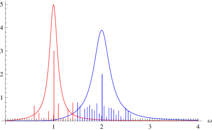
For $\Omega_{0}\gg 2\gamma_{0}$ (i.e., strongly underdamped regime) one can clearly see a spike in the vicinity of the oscillator frequency $2\Omega_{0}$ with the width of the spike being twice the width of $\tilde{S}(\omega)$ for the same parameters $\gamma_{0}$, $\Omega_{0}$.

It is straightforward to generalize the above discussion to generic observables of the form $A(\hat{X})$ using the Taylor expansion

$$A(\hat{X})=\sum_{n=0}^{\infty}\alpha_{n}\hat{X}^{n}.$$ (5.31)

After substituting this into the definition of the time correlator, and applying Wick’s thorem to the products of $X(t)$ we obtain

$$S_{A}(t)=\langle 0|A(\hat{X}(t))A(\hat{X})|0\rangle=\sum_{n=0}^{\infty}\beta_{n}S^{n}(t),$$ (5.32)

where $\beta_{n}$ are some coeficients having dimension of inverse length in power $2n$. Taking now the Fourier transform from both sides of this expression we obtain for the spectral function

$$\tilde{S}_{A}(\omega)=\frac{1}{2\pi}\int\limits_{-\infty}^{\infty}dt\,e^{it\omega}S_{A}(t)=\sum_{n=0}^{\infty}\beta_{n}\underbrace{\tilde{S}(\omega)*\tilde{S}(\omega)*\dots*\tilde{S}(\omega)}_{n\ {\rm times}}\ ,$$ (5.33)

where the symbol $*$ stands for the convolution. It is quickly seen that, in the underdamped regime, the $n$-th term of the sum (5.33) has a maximum at the vicinity of $n\Omega_{0}$ with a width given by $n\gamma$.

6 Conclusions

We studied collective behavior in an integrable model consisting of two coupled chains of harmonic oscillators. We chose the rescaled difference of the center of mass modes of the chains as a collective coordinate $X$, and mapped our system onto a model of Caldeira-Leggett type. The resemblance with the well-known Caldeira-Leggett model provides an intuitive physical picture of the energy exchange between the collective coordinate and the remaining degrees of freedom playing the role of the internal bath. As a result, the dynamics of the collective mode is described by the damped harmonic oscillator equation. We then relate this dynamical equation to the problem of the existence of collective quantum excitations in the spectrum of the corresponding quantum Hamiltonian. These collective excitations are probed through the transition strengths induced by observables $A(\hat{X})$, depending on the collective coordinate. As we show, for the dynamically underdamped regime the spikes in the distribution of the transition strengths appear precisely at the energies $E_{n}=E_{0}+n\hbar\Omega_{0}$ ($E_{0}=\mathrm{ground\ state\ energy}$) of the quantized collective harmonic oscillator, while the width of the spikes is controled by the damping coeficient $\gamma_{0}$ of the corresponding dynamical problem. It is worth mentioning that based on fluctuation-dissipation type of arguments we can extend the present approach to any Hamiltonian system with quadratic interactions.

One of the important features of our model is the freedom of choice for the collective coordinate. Note that our definition of $X$ in a technical sense was somewhat arbitrary. In principle, we could take any linear combination $Y=\sum_{i=1}^{N}\left(C_{i}x_{i}+\bar{C}_{i}\bar{x}_{i}\right)$ as a collective coordinate, and implement the same type of mapping procedure (as in the case of $X$) onto the model of Caldeira-Legget type. We would get then precisely the same equation of motion for $Y(t)$, but with a different collective frequency $\Omega_{0}$ and damping kernel $\gamma(t)$. Not every choice for $Y$ would be, of course, appropriate in order to regard it as a collective coordinate. If, for instance, the resulting dynamics becomes overdamped, no clear spikes will be visible at the corresponding spectral function. On the other hand, it seems that there exists no “unique” choice for the collective coordinate. This means the parameters $\Omega_{0}$, $\gamma_{0}$ are not intrinsic properties of the considered integrable model but are rather affected by the definition of the collective coordinate. It would be of a great interest to see whether and in what form the above “semiclassical” connection between the classical dynamics of a collective mode and collective excitations of the corresponding quantum problem can be extended to a more general class of non-integrable systems. It is clear that some substantial differences with an integrable case must arrise when the dynamics of the system becomes chaotic.

References

- [1] A. Bohr and B. Mottelson, Nuclear Structure, Vol. 1, W.A. Benjamin, INC (1969)
- [2] T.H. Oosterkamp, J.W. Janssen, L.P. Kouwenhoven, D.G. Austing, T. Honda and S. Tarucha, Phys. Rev. Lett. 82, 2931 (1999)
- [3] M. Toreblad, M. Borgh, M. Koskinen, M. Manninen and S.M. Reimann, Phys. Rev. Lett. 93, 090407 (2004)
- [4] D.A. Butts and D.S. Rokhsar, Nature 397, 327 (1999)
- [5] K.W. Madison, F. Chevy, W. Wohlleben and J. Dalibard, Phys. Rev. Lett. 84, 806 (2000)
- [6] O.M. Marago, S.A. Hopkins, J. Arlt, E. Hodby, G. Hechenblaikner and C.J. Foot, Phys. Rev. Lett. 84, 2056 (2000)
- [7] D. Clément, A.F. Varon, M. Hugbart, J. Retter, P. Bouyer, L. Sanchez–Palencia, D.M. Gangardt, G.V. Shlyapnikov and A. Aspect, Phys. Rev. Lett. 95, 170409 (2005)
- [8] C. Yannouleas and U. Landmann, Phys. Rev. Lett. 85, 1726 (2000)
- [9] T. Guhr, A. Müller–Groeling and H.A. Weidenmüller, Phys. Rep. 299, 189 (1998)
- [10] J. Enders, T. Guhr, N. Huxel, P. von Neumann–Cosel, C. Rangacharyulu and A. Richter, Phys. Lett. B486, 273 (2000)
- [11] J. Enders, T. Guhr, A. Heine, P. von Neumann–Cosel, V.Y. Ponomarev, A. Richter and J. Wambach, Nucl. Phys. A741, 3 (2004)
- [12] V.I. Arnold, Mathematical Methods of Classical Mechanics, Springer, Heidelberg (1978)
- [13] T. Papenbrock, Phys. Rev. C61, 034602 (2000)
- [14] V.V. Sokolov and V. Zelevinsky, Phys. Rev. C56, 311 (1997)
- [15] T. Guhr, Doorway Mechanism in Many–Body Systems and in Quantum Billiards, Acta Physica Polonica A, in press
- [16] M. Brack and R.K. Bhaduri, Semiclassical Physics, Frontiers in Physics 96, Addison-Wesley, Reading (1997)
- [17] A. O. Caldeira and A. J. Leggett, Physica A121, 587 (1983)
- [18] H. Kohler and F. Sols, Phys. Rev. B72, 180404 (2005)
- [19] H. Kohler and F. Sols, New J. Phys. 8, 149 (2006)
- [20] E. Lutz and H. A. Weidenmüller, Physica A267, 354 (1999)
- [21] H. Grabert, P. Schramm, and G.-L. Ingold, Phys. Rep. 168, 115 (1988)
- [22] F. Scheck, Mechanics: From Newton’s Laws to Deterministic Chaos, Springer, Heidelberg (2004)
- [23] A. Bulgac, G. D. Dang, D. Kusnezovc, Phys. Rev. E54 (1996) 3468
- [24] H.-P. Breuer and F. Petruccione, The Theory of Open Quantum Systems, Oxford University Press, Oxford (2002)
- [25] R. P. Feynman, Statistical Mechanics, Benjamin, New York (1972)