Feedback-dependent control of stochastic synchronization in coupled neural systems

Abstract

We investigate the synchronization dynamics of two coupled noise-driven FitzHugh-Nagumo systems, representing two neural populations. For certain choices of the noise intensities and coupling strength, we find cooperative stochastic dynamics such as frequency synchronization and phase synchronization, where the degree of synchronization can be quantified by the ratio of the interspike interval of the two excitable neural populations and the phase synchronization index, respectively. The stochastic synchronization can be either enhanced or suppressed by local time-delayed feedback control, depending upon the delay time and the coupling strength. The control depends crucially upon the coupling scheme of the control force, i.e., whether the control force is generated from the activator or inhibitor signal, and applied to either component. For inhibitor self-coupling, synchronization is most strongly enhanced, whereas for activator self-coupling there exist distinct values of the delay time where the synchronization is strongly suppressed even in the strong synchronization regime. For cross-coupling strongly modulated behavior is found.

1 Introduction

The control of unstable or irregular states of nonlinear dynamic systems has many applications in different fields of physics, chemistry, biology, and medicine [SCH07]. A particularly simple and efficient control scheme is time-delayed feedback [PYR92] which occurs naturally in a number of biological systems including neural networks where both propagation delays and local neurovascular couplings lead to time delays [HAK06, WIL99, GER02]. Moreover, time-delayed feedback loops might be deliberately implemented to control neural disturbances, e.g., to suppress undesired synchrony of firing neurons in Parkinson’s disease or epilepsy [SCH94e, ROS04a, POP05]. Here we study coupled neural systems subject to noise and time-delayed feedback [HAU06, HOE09, SCH08, SCH09a]. In particular we focus upon the question how stochastic synchronization of noise-induced oscillations of two coupled neural populations can be controlled by time-delayed feedback, and how robust this is with respect to different coupling schemes of the control force.

Time-delayed feedback control of noise-induced oscillations was demonstrated in a single excitable system [JAN03, BAL04, PRA07, POT08]. The simplest network configuration displaying features of neural interaction consists of two coupled excitable systems.

In order to grasp the complicated interaction between billions of neurons in large neural networks, those are often lumped into groups of neural populations each of which can be represented as an effective excitable element that is mutually coupled to the other elements [ROS04, POP05]. In this sense the simplest model which may reveal features of interacting neurons consists of two coupled neural oscillators. Each of these will be represented by a simplified FitzHugh-Nagumo (FHN) system [FIT60, NAG62], which is often used as a generic model for neurons, or more generally, excitable systems [LIN04].

This paper is organized as follow: We introduce the model equations and the feedback scheme in Sec. 2. Sec. 3 is devoted to two measures of the stochastic synchronization. These are investigated for different coupling schemes of the feedback in Sec. 4. Finally, we conlcude in Sec. 5.

2 Model Equations

Neurons are excitable units which can emit spikes or bursts of electrical signals, i.e., the system rests in a stable steady state, but after it is excited beyond a threshold, it emits a pulse. In the following, we consider electrically coupled neurons modelled by the FitzHugh-Nagumo system in the excitable regime:

$$\varepsilon_{1}\frac{du_{1}}{dt} = f\left(u_{1},v_{1}\right)+C\left(u_{2}-u_{1}\right)$$ (1a)

$$\frac{dv_{1}}{dt} = g\left(u_{1},v_{1}\right)+D_{1}\xi_{1}$$ (1b)

$$\varepsilon_{2}\frac{du_{2}}{dt} = f\left(u_{2},v_{2}\right)+C\left(u_{1}-u_{2}\right)$$ (2a)

$$\frac{dv_{2}}{dt} = g\left(u_{2},v_{2}\right)+D_{2}\xi_{2}$$ (2b)

with $f\left(u_{i},v_{i}\right)=u_{i}-u_{i}^{3}/3-v_{i}$ and $g\left(u_{i},v_{i}\right)=u_{i}+a$ ($i=1,2$). The fast activator variables $u_{i}$ ($i=1,2$) refer to the transmembrane voltage, and the slow inhibitor variables $v_{i}$ are related to the electrical conductance of the relevant ion currents. The parameter $a$ is the excitability parameter. For the purposes of this paper, $a$ is fixed at $1.05$, such that there are no autonomous oscillations (excitable regime). $C$ is the diffusive coupling strength between $u_{1}$ and $u_{2}$. To introduce different time scales for both systems, $\varepsilon_{1}$ is set to $0.005$ and $\varepsilon_{2}$ is set to $0.1$. Both systems, when uncoupled, are driven entirely by independent noise sources, which in the above equations are represented by $\xi_{i}$ ($i=1,2$, Gaussian white noise with zero mean and unity variance). $D_{i}$ is the noise intensity, and for the purposes of this paper, $D_{2}$ will be held fixed at $0.09$ [HAU06].

Figure 1: Schematic diagram of two coupled FitzHugh-Nagumo systems with time-delayed feedback applied to the first subsystem. $K$ and $\tau$ denote the feedback gain and time delay, respectively, and $C$ is the coupling strength.

The control force which we apply only to the first of the neural populations as schematically depicted in Fig. 1 is known as time-delay autosynchronization (TDAS) or time-delayed feedback control. This method was initially introduced by Pyragas [PYR92] for controlling periodic orbits in chaotic systems. It has been effective in a variety of experimental applications at controlling oscillatory behavior and can be easily implemented in many analog devices [SCH07]. TDAS constructs a feedback $F$ from the difference between the current value of a control signal $w$ and the value for that quantity at time $t-\tau$. The difference is then multiplied by the gain coefficient $K$

$$F(t)=K[w(t-\tau)-w(t)],$$ (3)

where $w$ determines which components of the system enter the feedback as will be discussed in the following.

The variable $w$ in the control force can be either the activator $u_{1}$ or the inhibitor $v_{1}$. Also, the control force can either be applied to the activator or the inhibitor differential equation. These possibilities lead to two self-coupling schemes ($uu$ and $vv$) where either the activator is coupled to the activator equation or the inhibitor is coupled to the inhibitor equation, and two cross-coupling schemes ($uv$ and $vu$). Thus, Eqs. (1) of the first subsystem can be rewritten including time-delayed feedback as

$$\left(\begin{array}[]{c}\varepsilon_{1}\frac{du_{1}}{dt}\\ \frac{dv_{1}}{dt}\end{array}\right) = \left(\begin{array}[]{c}f\left(u_{1},v_{1}\right)+C\left(u_{2}-u_{1}\right)\\ g\left(u_{1},v_{1}\right)+D_{1}\xi_{1}\end{array}\right)$$ (8)

$$+K\left(\begin{array}[]{cc}A_{uu}&A_{uv}\\ A_{vu}&A_{vv}\end{array}\right)\left(\begin{array}[]{c}u_{1}(t-\tau)-u_{1}(t)\\ v_{1}(t-\tau)-v_{1}(t)\\ \end{array}\right),$$ (13)

where the coupling matrix elements $A_{ij}$ with $i,j\in\{u,v\}$ define the specific coupling scheme.

Next, we will discuss cooperative stochastic dynamics resulting in frequency synchronization and phase synchronization in the following Sections.

3 Measures of Synchronization

A measure of frequency synchronization is the ratio of the interspike intervals (ISI) of the two neural populations [HAU06, HOE09]. The respective average ISI of each neural population is denoted by $\langle T_{1}\rangle$ and $\langle T_{2}\rangle$. The ratio $\langle T_{1}\rangle/\langle T_{2}\rangle$ compares the average time scales of both systems, where unity ratio describes two systems spiking at the same average frequency. It is for this reason that the ISI ratio is often considered as a measure of frequency synchronization. It does not contain information about the phase of synchronization, and a given ISI ratio can also result from different ISI distributions.

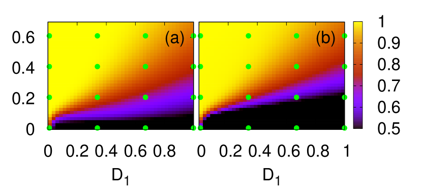
Figure 2: (Color online) Panels (a) and (b) show the ratio of interspike intervals $\langle T_{1}\rangle/\langle T_{2}\rangle$ and the phase synchronization index $\gamma$ of the two subsystems as color code in dependence on the coupling strength $C$ and noise intensity $D_{1}$, respectively. No control is applied to the system. The dots mark the parameter choice for different synchronization regimes used in the following. Other parameters: $\varepsilon_{1}=0.005$, $\varepsilon_{2}=0.1$, $a=1.05$, and $D_{2}=0.09$.

In order to account for the phase difference between two systems, one can define a phase [PIK96, PIK01, HAU06]

$$\varphi(t) = 2\pi\frac{t-t_{i-1}}{t_{i}-t_{i-1}}+2\pi(i-1)$$ (14)

where $i=1,2,\dots$. $t_{i}$ denotes the time of the $i$th spike. The phase difference between two consecutive spikes is $2\pi$. The phase difference of 1:1 synchronization is

$$\Delta\varphi(t) = \left|\varphi_{1}(t)-\varphi_{2}(t)\right|,$$ (15)

where $\varphi_{1}(t)$ and $\varphi_{2}(t)$ are the phases of the first and second system, respectively. Two systems that are phase synchronized at a given time satisfy $\Delta\varphi=0$. Finally, the overall time-averaged phase synchronization of two systems can be quantified using the synchronization index

$$\gamma=\sqrt{\langle\cos\Delta\varphi(t)\rangle^{2}+\langle\sin\Delta\varphi(t)\rangle^{2}}.$$ (16)

A value of $0$ indicates no synchronization, while a value of unity indicates perfect synchronization.

Figure 2 depicts both measures for stochastic synchronization in the $\left(D_{1},C\right)$ plane, both exhibiting very similar behavior. Panel (a) refers to the frequency synchronization characterized by the ratio of the average ISIs $\langle T_{1}\rangle/\langle T_{2}\rangle$ and panel (b) shows the phase synchronization index $\gamma$. The green dots mark parameter values used in Sec. 4. Note that both panels share the same color code. For a small value of $D_{1}$ and large coupling strength, the two subsystems display well synchronized behavior, $\langle T_{1}\rangle/\langle T_{2}\rangle\approx 1$ and $\gamma\approx 1$. The timescales in the interacting systems adjust themselves to $1:1$ synchronization. On average, they show the same number of spikes and the two subsystems are in-phase which is indicated by yellow color. The two subsystems are less synchronized in the dark blue and black regions.

In the following we show the ratio of the average interspike interval $\langle T_{1}\rangle/\langle T_{2}\rangle$ and the phase synchronization index $\gamma$ which are color coded in the $(\tau,K)$ plane for fixed combinations of $D_{1}$ and $C$. For each coupling scheme of time-delayed feedback control (cross-coupling schemes $uv$ and $vu$ and self-coupling schemes $uu$ and $vv$) we present a selection of $\left(D_{1},C\right)$ values. In all cases, only one element of the coupling matrix ${\bf A}$ is equal to unity and all other elements are zero.

4 Coupling Schemes

After the introduction of the system and the coupling schemes, we will present results on frequency and phase synchronization in the following. We consider $16$ different combinations of the noise intensity $D_{1}$ and the coupling strength $C$ which are marked as green dots in Fig. 2. The ordering of panels in Figs. 3 to 10 is the following: The rows correspond to fixed coupling strength chosen as $C=0.01,0.21,0.41$, and $0.61$ from bottom to top. The columns in each figure are calculated for constant noise intensity $D_{1}=0.01,0.34,0.67$, and $1.0$ from left to right.

4.1 Frequency Synchronization

Figures 3 to 6 show frequency synchronization measured by the ratio of average interspike intervals $\langle T_{1}\rangle/\langle T_{2}\rangle$ calculated from the summarized activator variable $u_{\Sigma}=u_{1}+u_{2}$ as color code in dependence on the feedback gain $K$ and the time delay $\tau$. The system’s parameters are fixed in each panel as described above. Figures 3 and 6 correspond to self-coupling ($uu$- and $vv$-coupling) and Figs. 4 and 5 depict the cross-coupling schemes ($uv$- and $vu$-coupling). The dynamics in the white regions is outside the excitable regime and does not show noise-induced spiking, but rather the system exhibits large-amplitude self-sustained oscillations.

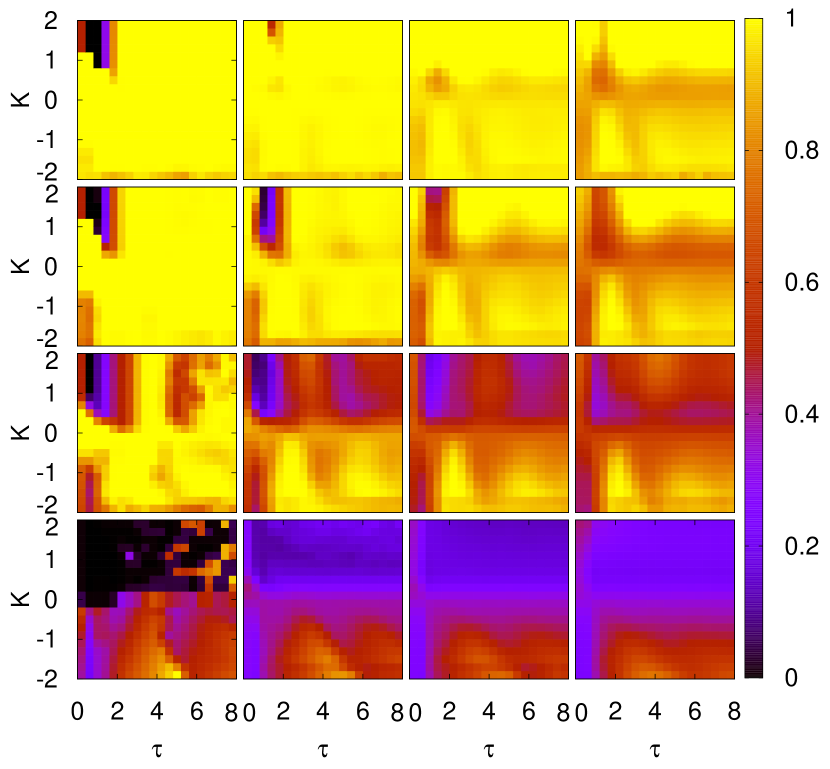
Figure 3: $uu$-coupling: Ratio of average interspike intervals $\langle T_{1}\rangle/\langle T_{2}\rangle$ as color code. Rows and columns correspond to constant coupling strength $C$ and noise intensity $D_{1}$, respectively, as marked in Fig. 2 as green dots, and specified in the text. Other parameters as in Fig. 2.

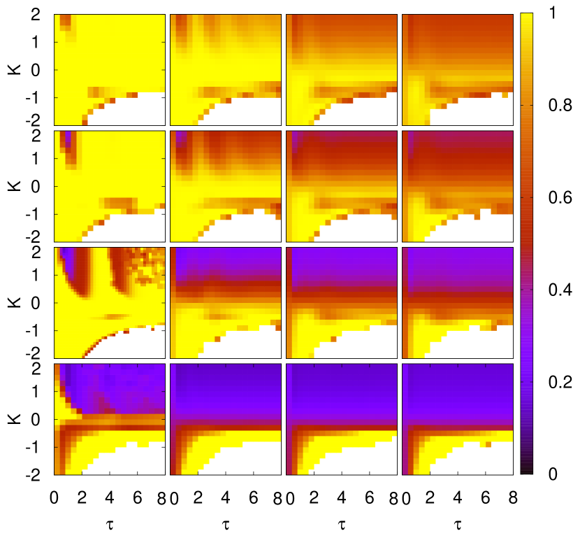
Figure 4: $uv$-coupling: Ratio of average interspike intervals $\langle T_{1}\rangle/\langle T_{2}\rangle$ as color code. Rows and columns correspond to constant coupling strength $C$ and noise intensity $D_{1}$, respectively. Other parameters as in Fig. 2.

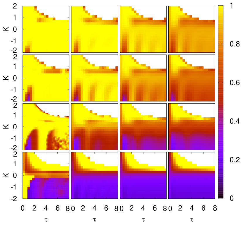
Figure 5: $vu$-coupling: Ratio of average interspike intervals $\langle T_{1}\rangle/\langle T_{2}\rangle$ as color code. Rows and columns correspond to constant coupling strength $C$ and noise intensity $D_{1}$, respectively. Other parameters as in Fig. 2.

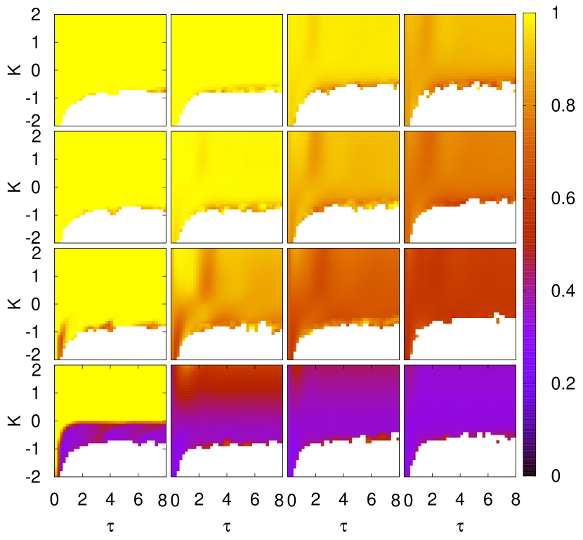
Figure 6: $vv$-coupling: Ratio of average interspike intervals $\langle T_{1}\rangle/\langle T_{2}\rangle$ as color code. Rows and columns correspond to constant coupling strength $C$ and noise intensity $D_{1}$, respectively. Other parameters as in Fig. 2.

One can see that appropriate tuning of the control parameters leads to enhanced or deteriorated synchronization displayed by bright yellow and dark blue areas, respectively. In each figure, all panels show qualitatively similar features like a modulation of the ratio $\langle T_{1}\rangle/\langle T_{2}\rangle$ whose range between maximum and minimum depends on $D_{1}$ and $C$. Comparing the rows, the systems are less (more strongly) synchronized for small (large) values of $C$ indicated by dark blue (yellow) color. As the noise intensity $D_{1}$ increases, the dynamics of the coupled subsystems is more and more noise-dominated and the dependence on the time delay $\tau$ becomes less pronounced.

Note the symmetry in the cross-coupling schemes shown as Figs. 4 and 5 between $K$ and its negative value $-K$ for the inverse cross-coupling. The reason is that enhancing the activator yields a similar effects on the dynamics as diminishing the inhibitor variable.

4.2 Phase Synchronization

Figures 7 to 10 depict the phase synchronization index $\gamma$ as color code depending on the control parameters $K$ and $\tau$ for $uu$-, $uv$-, $vu$-, and $vv$-coupling, respectively. The noise intensity $D_{1}$ and coupling strength $C$ are fixed for each panel as described in Sec. 4.1.

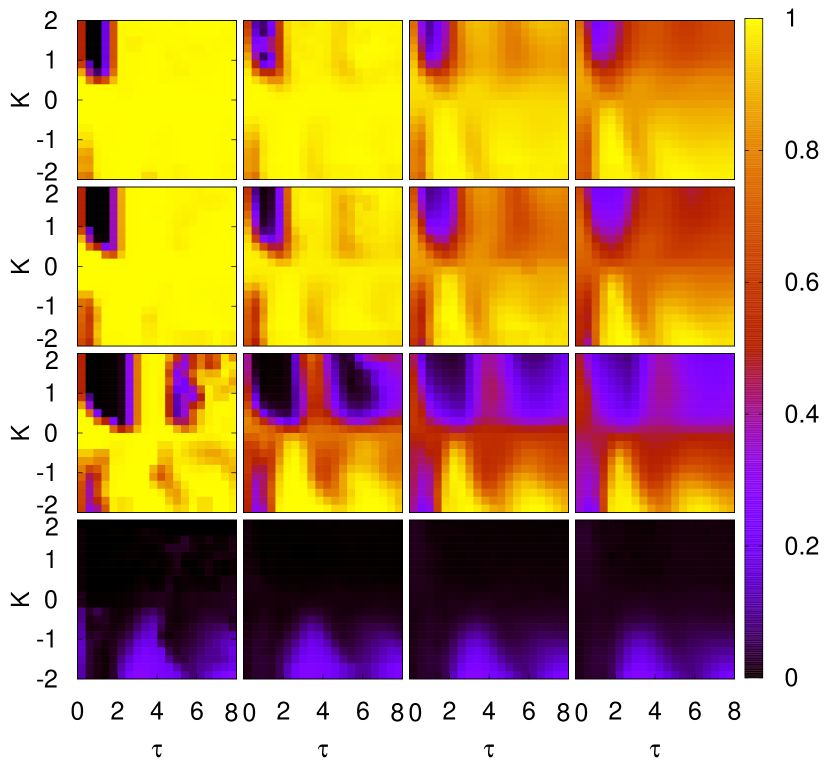
Figure 7: $uu$-coupling: Phase synchronization index $\gamma$. Noise intensity $D_{1}$ and coupling strength $C$ chosen as described in Sec. 4.1. Other parameters as in Fig. 2.

Comparing Figs. 7 to 10 with the respective plots for frequency synchronization, i.e., Figs. 3 to 6, one can see that both types of synchronization coincide qualitatively, but the phase synchronization index is more sensitive to the modulation features. Similar to the case of frequency synchronization, time delayed feedback can lead to either enhancement or suppression of phase synchronization depending on the specific choice of the feedback gain $K$ and time delay $\tau$ indicated by yellow and dark blue regions. In general, these effects become less sensitive on the time delay as $D_{1}$ increases. For larger values of $C$, the two subsystems show enhanced phase synchronization.

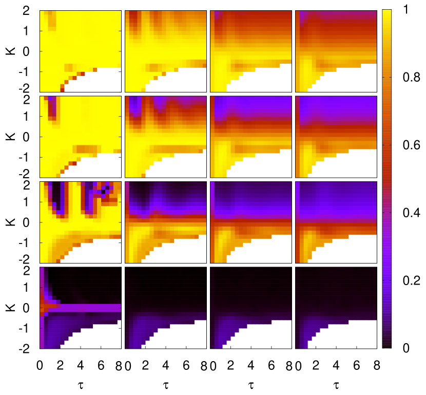
Figure 8: $uv$-coupling: Phase synchronization index $\gamma$. Noise intensity $D_{1}$ and coupling strength $C$ chosen as described in Sec. 4.1. Other parameters as in Fig. 2.

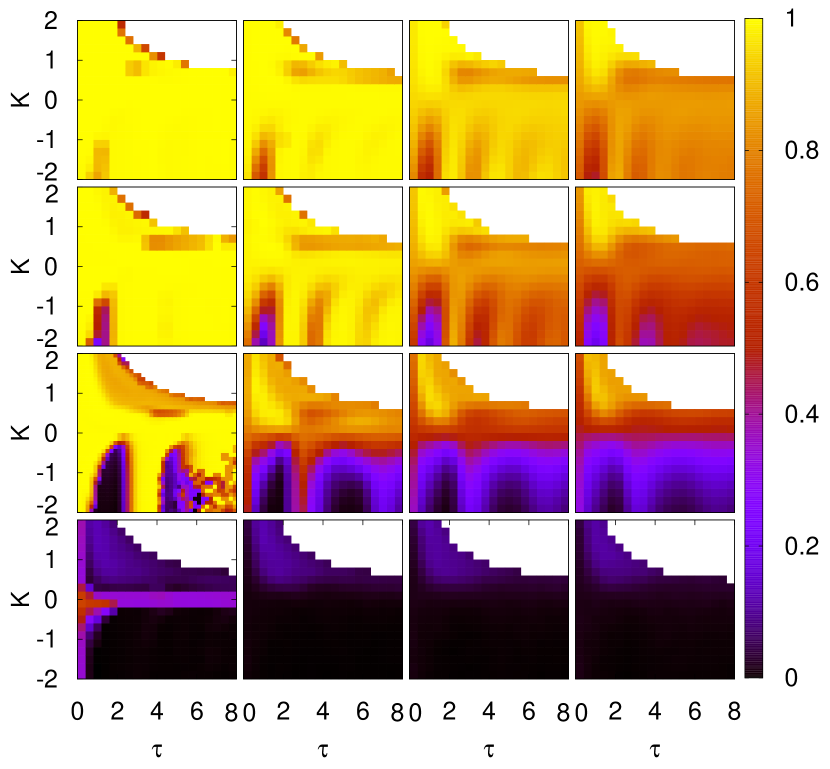
Figure 9: $vu$-coupling: Phase synchronization index $\gamma$. Noise intensity $D_{1}$ and coupling strength $C$ chosen as described in Sec. 4.1. Other parameters as in Fig. 2.

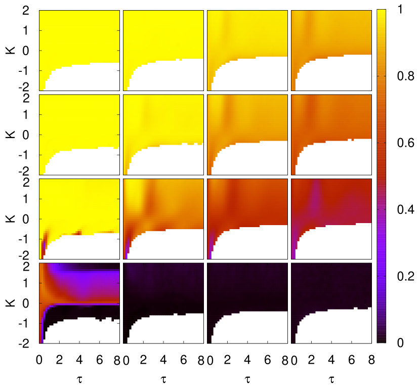
Figure 10: $vv$-coupling: Phase synchronization index $\gamma$. Noise intensity $D_{1}$ and coupling strength $C$ chosen as described in Sec. 4.1. Other parameters as in Fig. 2.

5 Conclusion

In summary, we have shown that stochastic synchronization in two coupled neural populations can be tuned by local time-delayed feedback control of one population. Synchronization can be either enhanced or suppressed, depending upon the delay time and the coupling strength. The control dependents crucially upon the coupling scheme of the control force. For inhibitor self-coupling ($vv$) synchronization is most strongly enhanced, whereas for activator self-coupling ($uu$) there exist distinct values of $\tau$ where the synchronization is strongly suppressed even in the strong synchronization regime. For cross-coupling ($uv$, $vu$) there is mixed behavior, and both schemes exhibit a strong symmetry with respect to inverting the sign of $K$. These observations might be important in the context of the deliberate application of control with the aim of suppressing synchronization, e.g. as therapeutic measures for Parkinson’s disease.

References

- [1] \harvarditem[Balanov et al.]Balanov et al.2004BAL04 Balanov, A. G., N. B. Janson and E. Schöll (2004). Control of noise-induced oscillations by delayed feedback. Physica D 199, 1–12.
- [2] \harvarditem[FitzHugh]FitzHugh1960FIT60 FitzHugh, R. (1960). Thresholds and plateaus in the Hodgkin-Huxley nerve equations. J. Gen. Physiol. 43(5), 867–896.
- [3] \harvarditem[Gerstner and Kistler]Gerstner and Kistler2002GER02 Gerstner, W. and W. Kistler (2002). Spiking neuron models. Cambridge University Press. Cambridge.
- [4] \harvarditem[Haken]Haken2006HAK06 Haken, H. (2006). Brain Dynamics: Synchronization and Activity Patterns in Pulse-Coupled Neural Nets with Delays and Noise. Springer Verlag GmbH. Berlin.
- [5] \harvarditem[Hauschildt et al.]Hauschildt et al.2006HAU06 Hauschildt, B., N. B. Janson, A. G. Balanov and E. Schöll (2006). Noise-induced cooperative dynamics and its control in coupled neuron models. Phys. Rev. E 74, 051906.
- [6] \harvarditem[Hövel et al.]Hövel et al.2009HOE09 Hövel, P., M. A. Dahlem and E. Schöll (2009). Control of synchronization in coupled neural systems by time-delayed feedback. Int. J. Bifur. Chaos (in print). (arxiv:0809.0819v1).
- [7] \harvarditem[Janson et al.]Janson et al.2004JAN03 Janson, N. B., A. G. Balanov and E. Schöll (2004). Delayed feedback as a means of control of noise-induced motion. Phys. Rev. Lett. 93, 010601.
- [8] \harvarditem[Lindner et al.]Lindner et al.2004LIN04 Lindner, B., J. García-Ojalvo, A. Neiman and Lutz Schimansky-Geier (2004). Effects of noise in excitable systems. Phys. Rep. 392, 321–424.
- [9] \harvarditem[Nagumo et al.]Nagumo et al.1962NAG62 Nagumo, J., S. Arimoto and S. Yoshizawa. (1962). An active pulse transmission line simulating nerve axon.. Proc. IRE 50, 2061–2070.
- [10] \harvarditem[Pikovsky et al.]Pikovsky et al.1996PIK96 Pikovsky, A., M. G. Rosenblum and J. Kurths (1996). Synchronisation in a population of globally coupled chaotic oscillators. Europhys. Lett. 34, 165.
- [11] \harvarditem[Pikovsky et al.]Pikovsky et al.2001PIK01 Pikovsky, A., M. G. Rosenblum and J. Kurths (2001). Synchronization, A Universal Concept in Nonlinear Sciences. Cambridge University Press. Cambridge.
- [12] \harvarditem[Popovych et al.]Popovych et al.2005POP05 Popovych, O. V., C. Hauptmann and Peter A. Tass (2005). Effective desynchronization by nonlinear delayed feedback. Phys. Rev. Lett. 94, 164102.
- [13] \harvarditem[Pototsky and Janson]Pototsky and Janson2008POT08 Pototsky, Andrey and N. B. Janson (2008). Excitable systems with noise and delay, with applications to control: Renewal theory approach. Phys. Rev. E 77(3), 031113.
- [14] \harvarditem[Prager et al.]Prager et al.2007PRA07 Prager, T., H. P. Lerch, Lutz Schimansky-Geier and E. Schöll (2007). Increase of coherence in excitable systems by delayed feedback. J. Phys. A 40, 11045–11055.
- [15] \harvarditem[Pyragas]Pyragas1992PYR92 Pyragas, K. (1992). Continuous control of chaos by self-controlling feedback. Phys. Lett. A 170, 421.
- [16] \harvarditem[Rosenblum and Pikovsky]Rosenblum and Pikovsky2004aROS04a Rosenblum, M. G. and A. Pikovsky (2004a). Controlling synchronization in an ensemble of globally coupled oscillators. Phys. Rev. Lett. 92, 114102.
- [17] \harvarditem[Rosenblum and Pikovsky]Rosenblum and Pikovsky2004bROS04 Rosenblum, M. G. and A. Pikovsky (2004b). Delayed feedback control of collective synchrony: An approach to suppression of pathological brain rhythms. Phys. Rev. E 70, 041904.
- [18] \harvarditem[Schiff et al.]Schiff et al.1994SCH94e Schiff, S. J., K. Jerger, D. H. Duong, T. Chang, M. L. Spano and W. L. Ditto (1994). Controlling chaos in the brain. Nature (London) 370, 615.
- [19] \harvarditem[Schöll and Schuster]Schöll and Schuster2008SCH07 Schöll, E. and Schuster, H. G., Eds.) (2008). Handbook of Chaos Control. Wiley-VCH. Weinheim. Second completely revised and enlarged edition.
- [20] \harvarditem[Schöll et al.]Schöll et al.2009aSCH08 Schöll, E., G. Hiller, P. Hövel and M. A. Dahlem (2009a). Time-delayed feedback in neurosystems. Phil. Trans. R. Soc. A 367, 1079–1096.
- [21] \harvarditem[Schöll et al.]Schöll et al.2009bSCH09a Schöll, E., P. Hövel, V. Flunkert and M. A. Dahlem (2009b). Time-delayed feedback control: from simple models to lasers and neural systems. In: Complex Time-Delay Systems (F. M. Atay, Ed.). Springer. Berlin.
- [22] \harvarditem[Wilson]Wilson1999WIL99 Wilson, H. R. (1999). Spikes, Decisions, and Actions: The Dynamical Foundations of Neuroscience. Oxford University Press. Oxford.
- [23]