Inhomogeneous phases of strongly interacting matter

Abstract

We discuss possible inhomogeneous phases in two regions of the QCD phase diagram: We begin with color superconducting quark matter at moderately high densities, which is an imbalanced Fermi system due to the finite strange quark mass and neutrality constraints. Within an NJL-type toy model we find that this situation could lead to the formation of a soliton lattice. Similar solutions also exist in the context of the chiral phase transition. As an interesting result, the first-order transition line in the phase diagram of homogeneous phases gets replaced by an inhomogeneous phase which is bordered by two second-order transition lines.

12.38.Mh

1 Introduction

The phase structure of QCD is one of the most fascinating problems in the field of strong interaction physics. So far, most studies have been performed under the assumption that the condensates which define the different phases are homogeneous. On the other hand, there are good arguments to believe that there could be inhomogeneous phases as well. Well known examples from the literature are, for instance, the chiral density wave [1, 2], the Skyrme crystal [3], and crystalline color superconductors [4, 5, 6, 7, 8]. They also emerge in the large $N$-limit of the $1+1$ dimensional Gross-Neveu model [9, 10].

In the main part of this talk we concentrate on color superconductors. In BCS theory, pairing occurs among fermions with opposite momenta, forming Cooper pairs with zero total momentum. If both fermions are at their respective Fermi surface, the pair can be created at no free-energy cost and the pairing is always favored as soon as there is an attractive interaction. This is, however, no longer the case if the Fermi momenta of the fermions to be paired are unequal. This situation arises naturally in quark matter as a consequence of the heavier strange quark mass and requirements of neutrality and beta equilibrium [11, 12]. BCS pairing then requires that the Fermi spheres first have to be equalized. This could be realized, e.g., in a weak process which replaces some of the down quarks by strange quarks. Of course, it will only be favorable if the free energy which is needed for this process is overcompensated by the pairing energy. Consequently there is a limit for this mechanism in terms of the Fermi momentum difference in the unpaired system and the BCS gap [13].

An alternative option is then that the matter becomes inhomogeneous [14, 15, 16]. The basic idea is to form Cooper pairs with non-zero total momentum. This has the obvious advantage that the fermions in the pair no longer have to have opposite momenta, and therefore each of them can stay on its respective Fermi surface. In the context of color superconductors, this possibility has been investigated first in Ref. [4]. The authors restricted themselves to a plane-wave ansatz for the gap function, as suggested first by Fulde and Ferrell (FF) in the context of metallic superconductors [14].

On the other hand, since in the FF ansatz the total momentum of the pair is restricted to a non-zero but constant value, this pairing pattern is strongly disfavored by phase space in most cases. One should therefore consider a multiple plane wave ansatz, as originally suggested by Larkin and Ovchinnikov (LO) [15]. In the context of color superconductors, this was discussed, e.g., in Refs. [5, 6, 7, 8]. As expected, the resulting solutions were found to be strongly favored against the FF phase. However, these analyses were restricted to a Ginzburg-Landau approximation. Moreover, the crystal structures have been restricted to superpositions of a finite number of plane waves whose wave vectors all have the same length, whereas one should also allow for the superposition of different wave lengths. A first step to overcome these shortcomings was done in Ref. [17] where inhomogeous pairing was studied within an NJL model. The main ideas of this paper will be discussed in Sec. 2.

More recently, the idea of having inhomogeneous phases in the context of the chiral phase transition was revisited in Refs. [18, 19] for the NJL model. In this case the transition from a dynamically broken to the chirally restored phase when increasing the chemical potential is delayed by the formation of an inhomogeneous chirally broken ground state. Also the orders of the phase transitions are modified. This will be discussed briefly in Sec. 3.

2 Inhomogeneous color superconductivity

2.1 Model

We consider an NJL-type Lagrangian for massless quarks $q$ with three flavor and three color degrees of freedom,

$$\mathcal{L}=\bar{q}\,(i{\partial/}+\hat{\mu}\gamma^{0})\,q+\mathcal{L}_{\mathit{int}}\,,$$ (1)

where $\hat{\mu}$ is the diagonal matrix of chemical potentials. The interaction term is given by

$$\mathcal{L}_{\mathit{int}}=H\sum_{A,A^{\prime}=2,5,7}(\bar{q}\,i\gamma_{5}\tau_{A}\lambda_{A^{\prime}}\,q_{C})(\bar{q}_{C}\,i\gamma_{5}\tau_{A}\lambda_{A^{\prime}}\,q)\,.$$ (2)

Here $H$ is a dimensionful coupling constant and $q_{C}(x)=C\bar{q}^{T}(x)$, where $C=i\gamma^{2}\gamma^{0}$ is the matrix of charge conjugation. $\tau_{A}$ and $\lambda_{A^{\prime}}$ denote the antisymmetric Gell-Mann matrices acting in flavor space and color space, respectively. Thus, $\mathcal{L}_{\mathit{int}}$ corresponds to a quark-quark interaction in the scalar flavor-antitriplet color antitriplet channel. Applying standard bosonization techniques, the interaction term, can equivalently be rewritten as

$$\mathcal{L}_{\mathit{int}}=\frac{1}{2}\sum_{A,A^{\prime}}\Big{\{}\;(\bar{q}\,\gamma_{5}\tau_{A}\lambda_{A^{\prime}}\,q_{C})\;\varphi_{AA^{\prime}}\;+\;h.c.\;-\,\frac{1}{2H}\,\varphi_{AA^{\prime}}^{\dagger}\,\varphi_{AA^{\prime}}\Big{\}},$$ (3)

with the auxiliary complex boson fields $\varphi_{AA^{\prime}}(x)$, which, by the equations of motion, $\varphi_{AA^{\prime}}(x)=-2H\,\bar{q}_{C}(x)\,\gamma_{5}\tau_{A}\lambda_{A^{\prime}}\,q(x)$, can be identified with scalar diquarks. In mean field approximation we replace these quantum fields by their expectation values

$$\langle{\,\varphi_{AA^{\prime}}(x)}\rangle=\Delta_{A}(x)\,\delta_{AA^{\prime}}\,,$$ (4)

where the “gap function” $\Delta_{A}(x)$ is now a classical field. Here we assume that the condensation takes place only in the diagonal flavor-color components of the gap matrix, $A=A^{\prime}$, as in the standard ansatz for the CFL or the 2SC phase. Note, however, that we retain the full space-time dependence of the field. Introducing Nambu-Gor’kov bispinors, $\Psi(x)=\frac{1}{\sqrt{2}}\left(q(x),q_{C}(x)\right)^{T}$ and the notation $\hat{\Delta}(x)=\sum_{A}\Delta_{A}(x)\,\tau_{A}\lambda_{A}$, we obtain the effective mean-field Lagrangian

$$\mathcal{L}_{\mathit{MF}}(x)=\bar{\Psi}(x)\,S^{-1}(x)\,\Psi(x)\,-\,\frac{1}{4H}\sum_{A}|\Delta_{A}(x)|^{2}\,,$$ (5)

with the inverse dressed quark propagator

$$S^{-1}(x)=\left(\begin{array}[]{cc}i{\partial/}+\hat{\mu}\gamma^{0}&\hat{\Delta}(x)\,\gamma_{5}\\ -\hat{\Delta}^{*}(x)\,\gamma_{5}&i{\partial/}-\hat{\mu}\gamma^{0}\end{array}\right)\,.$$ (6)

Since $\mathcal{L}_{\mathit{MF}}$ is bilinear in the Nambu-Gor’kov fields, they can formally be integrated out and we obtain the mean-field thermodynamic potential per volume $V$

$$\Omega_{MF}(T,\hat{\mu})\,=\,-\frac{1}{2}\frac{T}{V}\mathrm{Tr}\ln\,\frac{S^{-1}}{T}\,+\,\frac{T}{V}\sum\limits_{A}\int\limits_{[0,\frac{1}{T}]\otimes V}d^{4}x\;\frac{|\Delta_{A}(x)|^{2}}{4H}\,.$$ (7)

Note, however, that the evaluation of the functional $\mathrm{Tr}\ln$ is highly nontrivial because of the $x$ dependent gap functions.

To proceed, we assume that the gap matrix $\hat{\Delta}(x)$ is time independent and periodic in space, $\hat{\Delta}(x)\equiv\hat{\Delta}(\vec{x})=\hat{\Delta}(\vec{x}+\vec{a}_{i})$, $i=1,2,3$. Hence, $\hat{\Delta}$ can be decomposed into a discrete set of Fourier components

$$\hat{\Delta}(x)=\sum_{q_{k}}\hat{\Delta}_{q_{k}}\,e^{-iq_{k}\cdot x}\,,$$ (8)

where the allowed momenta $q_{k}=(0,\vec{q}_{k})$ form a reciprocal lattice in momentum space. The inverse propagator is then a matrix whose momentum components are given by

$$S^{-1}_{p_{m},p_{n}}=\left(\begin{array}[]{cc}({p/}_{n}+\hat{\mu}\gamma^{0})\,\delta_{p_{m},p_{n}}&\sum_{q_{k}}\hat{\Delta}_{q_{k}}\gamma_{5}\,\delta_{q_{k},p_{m}-p_{n}}\\ -\sum_{q_{k}}\hat{\Delta}^{*}_{q_{k}}\gamma_{5}\,\delta_{q_{k},p_{n}-p_{m}}&({p/}_{n}-\hat{\mu}\gamma^{0})\,\delta_{p_{m},p_{n}}\end{array}\right)\,.$$ (9)

Note that in general $S^{-1}$ is not diagonal in momentum space because the condensates $\hat{\Delta}_{q_{k}}$ couple different momenta. Physically, this corresponds to processes like the absorption of a hole with momentum $p_{n}$ by the condensate together with the emission of a quark with momentum $p_{m}=p_{n}+q_{k}$. This is only possible because the inhomogeneous diquark condensates carry momentum. In the homogeneous case, $\hat{\Delta}(x)=\mathit{const.}$, only the momentum component $q_{k}=0$ exists, and the in- and outgoing quark momenta are equal. While this is no longer true for our inhomogeneous ansatz, the fact that we consider a static solution still guarantees that the energy of the quark is conserved. This means, $S^{-1}$ is still diagonal in the Matsubara frequencies $\omega_{p_{n}}$, which can therefore be summed in the usual way. To that end we write

$$S^{-1}_{p_{m},p_{n}}=\gamma^{0}\,(i\omega_{p_{n}}-{\cal H}_{\vec{p}_{m},\vec{p}_{n}})\,\delta_{\omega_{p_{m}},\omega_{p_{n}}},$$ (10)

defining the effective Hamilton operator ${\cal H}$, which does not depend on $\omega_{p_{n}}$. Since ${\cal H}$ is hermitian, it can in principle be diagonalized. In this context it is important that, since the momenta $\vec{q}_{k}$ of the condensates form a reciprocal lattice, not all momentum components are coupled with each other, but ${\cal H}$ is block diagonal with one block ${\cal H}(\vec{k})$ for each vector $\vec{k}$ in the Brioullin zone ($B.Z.$). We then finally obtain for the thermodynamic potential

$$\Omega_{MF}=-\frac{1}{4}\int\limits_{B.Z.}\frac{d^{3}k}{(2\pi)^{3}}\sum\limits_{\lambda}\left[E_{\lambda}(\vec{k})+2T\,\ln\left(1+2e^{-E_{\lambda}(\vec{k})/T}\right)\right]\,+\sum\limits_{A}\sum\limits_{q_{k}}\frac{|\Delta_{A,q_{k}}|^{2}}{4H},$$ (11)

where $E_{\lambda}(\vec{k})$ are the eigenvalues of ${\cal H}(\vec{k})$. Here one should note that ${\cal H}(\vec{k})$ is not only an infinite matrix in momentum space, but each momentum component is also a $72\times 72$ matrix corresponding to 4 Dirac, 3 color, 3 flavor, and 2 Nambu-Gor’kov components. The numerical studies below are therefore performed in a simplified model, where the main focus is on the new features related to the inhomogeneity. To that end we consider a 2SC-like pairing scheme, where only two flavors (“up” and “down”) and two colors (“red” and “green”) are paired, so that the remaining ones (“strange” and “blue”) decouple. We assume that the chemical potentials may be different for up and down quarks,

$$\mu_{u}=\bar{\mu}+\delta\mu~{},\quad\mu_{d}=\bar{\mu}-\delta\mu~{},$$ (12)

but do not depend on color. Furthermore, we simplify the Dirac structure via a high-density approximation (see Ref. [17] for details). The problem is then reduced to diagonalize an effective Hamiltonian whose momentum components are only $2\times 2$ matrices,

$$({\cal H}_{\Delta,\delta\mu})_{\vec{p}_{m},\vec{p}_{n}}=\left(\begin{array}[]{cc}(p_{m}-\bar{\mu}-\delta\mu)\,\delta_{\vec{p}_{m},\vec{p}_{n}}&\Delta_{p_{m}-p_{n}}\\ \Delta^{*}_{p_{n}-p_{m}}&-(p_{m}-\bar{\mu}+\delta\mu)\,\delta_{\vec{p}_{m},\vec{p}_{n}}\end{array}\right)~{}.$$ (13)

Finally, we should note that the thermodynamic potential as defined in Eq. (11) is divergent and needs to be regularized. As discussed in Ref. [17], a restriction of the momenta of the effective Hamiltonian, which would be a straight forward generalization of the standard momentum cutoff in homogeneous phases, leads to strong regularization artifacts. We therefore suggest a Pauli-Villars like regularization scheme, where the regulator terms are given by replacing the free-energy eigenvalues $E_{\lambda}$ by $E_{\lambda,j}=\sqrt{E_{\lambda}^{2}+j\Lambda^{2}}$.

2.2 Numerical results for one-dimensional periodic structures

In the following, we restrict ourselves to $T=0$ and to a fixed average chemical potential $\bar{\mu}=400$ MeV, so that $\delta\mu$ is the only remaining external variable. Our model has two parameters, namely the coupling constant $H$ and the cutoff parameter $\Lambda$. Having fixed the cutoff, we can express the coupling constant $H$ through the corresponding value of the BCS gap at $\delta\mu=0$. The examples shown below correspond to $\Lambda=400$ MeV and $\Delta_{BCS}=80$ MeV. We remind that $\Lambda$ restricts the free energies and not the momenta. Thus, the most relevant excitations around the Fermi surface are always included, and there is no need for $\Lambda$ to be larger than the chemical potential.

Our goal is to find the most stable solution, i.e., the minimum of $\Omega$ with respect to the gap function $\Delta(\vec{x})$. Since the general solution of this problem is rather difficult, we restrict ourselves to one dimensional modulations, i.e., to gap functions which vary periodically in one spatial direction ($z$-direction), but stay constant in the two spatial directions ($x$ and $y$),

$$\Delta(z)=\sum_{k}\Delta_{q,k}e^{2ikqz}\,.$$ (14)

Moreover, we assume that $\Delta(z)$ is real, $\Delta_{q,k}^{*}=\Delta_{q,-k}$.

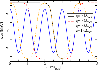
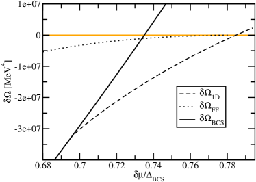
Figure 1: Left: The gap function in coordinate space at $\delta\mu=0.7\Delta_{BCS}$ for different fixed values of $q$. Right: Difference between the thermodynamic potentials of different solutions and the normal phase as functions of $\delta\mu$: BCS phase (solid line), general one-dimensional ansatz (dashed line), and single plane wave (FF) ansatz (dotted line). From Ref. [17].

In a first step, we take a fixed period, i.e., a fixed value of $q$ and minimize the thermodynamic potential with respect to the Fourier components $\Delta_{q,k}$. In the left panel of Fig. 1 we present examples we obtained for $\delta\mu=0.7\Delta_{\mathit{BCS}}$. At $q\sim\Delta_{BCS}$ the gap function appears to be sinusoidal. For larger periods, however, a new feature becomes apparent: the formation of a soliton lattice. Especially for $q=0.1\,\Delta_{\mathit{BCS}}$, we see that the gap function stays nearly constant at $\pm\Delta_{BCS}$ for about one half-period and then changes its sign in a relatively small interval. The $q=0.2\,\Delta_{\mathit{BCS}}$ solution behaves qualitatively similar, but has a shorter plateau. Remarkably, the shape of the two functions is almost identical in the transition region where the gap functions change sign. This remains even true for the $q=0.5\,\Delta_{\mathit{BCS}}$ solution, which is kind of an extreme case with no plateau and only transition regions. We may thus interprete these transition regions as very weakly interacting solitons, which are almost unaffected by the presence of the neighboring (anti-) solitons as long as they do not overlap.

It turns out that the gap functions can be fitted remarkably well by Jacobi elliptic functions, $\Delta_{\mathrm{fit}}(z)=A\,\mathrm{sn}\big{(}\kappa(z-z_{0});\nu\big{)}$, which is the known shape of the gap functions in $1+1$ dimensions [20] (see Eq. (15) below). An important difference is, however, that in $3+1$ dimensions the amplitude $A$ is not directly related to the elliptic modulus $\nu$, but must be fitted independently.

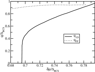
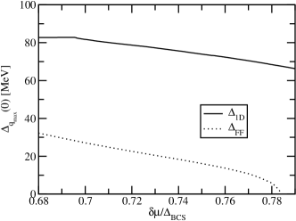
Figure 2: The energetically preferred value of $q$ (left) and the corresponding amplitude of the gap function (right) as functions of $\delta\mu$. Solid line: general one-dimensional ansatz, dotted line: single plane wave (FF) ansatz. From Ref. [17].

For each $\delta\mu$, with the solutions for the different chosen values of $q$ at hand, we now have to minimize the thermodynamic potential in $q$. The resulting free energy gain compared to the normal conducting solution is shown in the right panel of Fig. 1. While the BCS solution (solid line) and the normal solution are favored at low and high $\delta\mu$, respectively, there is a window at intermediate $\delta\mu$ where the inhomogeneous solution is favored. Note that for the general one-dimensional ansatz (dashed line), this window is about twice as wide as it would be for the single plane-wave ansatz (FF phase, dotted), which is energetically much less favored. Most striking, whereas the BCS-FF phase transition would be first order, the transition from the BCS phase to the general one-dimensional phase is second order. This is possible because the most favored value of $q$ in the inhomogeneous phase goes continuously to zero, when $\delta\mu$ is reduced towards the phase boundary, see left panel of Fig. 2 (solid line). The corresponding amplitude of the gap function is displayed on the right-hand side of Fig. 2. Unlike the FF amplitude (dotted), the amplitude of the general one-dimensional gap function stays of the order of $\Delta_{\mathit{BCS}}$ at large $\delta\mu$. As a consequence, the phase transition to the normal phase is first order. The resulting behavior of the gap function with increasing $\delta\mu$ is sketched in Fig. 3.

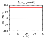
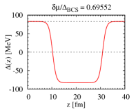
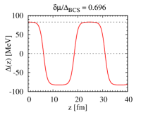
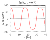
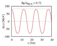
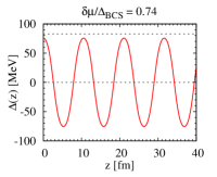
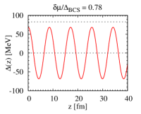
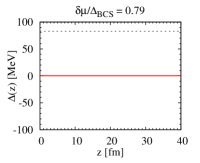
Figure 3: The color superconducting gap function in coordinate space for different values of $\delta\mu$ and the corresponding most favored value of $q$.

3 Chiral Phase transition

More recently, a similar study of inhomogeneous phases has been performed for the chiral phase transition [18, 19]. Here, instead of the color superconducting gap, the chiral condensate or, equivalently, the “constituent quark mass” was allowed to have general one-dimensional periodic modulations. This case actually turned out to be simpler, because it can be shown that the analytically known mass functions

$$M_{1+1}(z)=\sqrt{\nu}\kappa\,\mathrm{sn}\big{(}\kappa(z-z_{0});\nu\big{)}$$ (15)

of the $1+1$ dimensional Gross-Neveu model [9] can be lifted to $3+1$ dimensions by Lorentz boosts [19]. Apart from the irrelevant shift $z_{0}$, this function depends only on two parameters $\kappa$ and $\nu$, which are related to the wave vector $q=\pi\kappa/4K(\nu)$ ($K(\nu)=$ complete elliptic integral of the first kind) and the amplitude $\sqrt{\nu}\kappa$. Thus, at each temperature and chemical potential, the thermodynamic potential must be minimized w.r.t. $\kappa$ and $\nu$.

The resulting phase diagram for a two-flavor NJL model in the chiral limit is shown in the left panel of Fig. 4. When the solutions are restricted to homogeneous condensates, the phase transition is first order at lower temperatures (red long-dashed line) and second order at higher temperatures (black dotted line). However, when inhomogeneous condensates are taken into account, the first-order phase boundary becomes completely hidden by an inhomogeneous phase (orange shaded region). The latter is bordered by two second-order boundaries, whose intersection defines a Lifshitz point. In the NJL model the Lifshitz point precisely agrees with the critical point [18], similar to the findings in the Gross-Neveu model.

On the r.h.s. of Fig. 4, we display the wave vector $|\vec{q}|$ (dashed line) and the average amplitude of the mass function (solid line) as functions of the chemical potential $\mu_{q}$ at $T=0$. Similar to the superconducting case, $|\vec{q}|$ goes to zero at the lower end of the inhomogeneous phase, so that the latter is continuously connected to the homogeneous phase with broken chiral symmetry. At the upper end, the amplitude goes to zero, and the inhomogeneous phase is smoothly connected to the chirally restored phase.

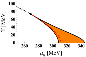
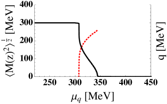
Figure 4: Left: Phase diagram in the chiral limit. The orange shaded region marks the inhomogeneous regime. Right: Wave vector $|\vec{q}|$ (dashed line) and average amplitude $\sqrt{\langle M^{2}\rangle}$ (solid line) at $T=0$ as functions of the quark chemical potential $\mu_{q}$. Adapted from Ref. [19].

4 Outlook

The results presented here should be considered as first steps towards a more complete picture of the phase diagram with inhomogeneous phases, and much remains to be done. In the context of the chiral phase transition one should couple the quarks to the Polyakov loop and study the influence of other interaction channels [21]. On the color-superconductivity side, one should calculate the equation of state for globally neutral quark matter in beta equilibrium and extend the analysis to finite temperature. Eventually, superconducting and chiral condensates should be treated simultaneously to obtain a unified phase diagram. Moreover, the model should be extended to $2+1$ flavors.

The restriction to inhomogeneities with one-dimensional modulations should not be the last word, but it would be interesting to study two- or even three-dimensional modulations as well. Technically, this is of course much more demanding. Eventually, however, one would like to study the transition from a single nucleon (described as a single soliton [22, 23]) to nuclear matter and finally to color-superconducting quark matter.

References

- [1] W. Broniowski, A. Kotlorz and M. Kutschera, Acta Phys. Polon. B 22, 145 (1991).
- [2] E. Nakano and T. Tatsumi, Phys. Rev. D 71, 114006 (2005).
- [3] A. S. Goldhaber and N. S. Manton, Phys. Lett. B 198, 231 (1987).
- [4] M. G. Alford, J. A. Bowers and K. Rajagopal, Phys. Rev. D 63, 074016 (2001).
- [5] J. A. Bowers and K. Rajagopal, Phys. Rev. D 66, 065002 (2002).
- [6] R. Casalbuoni, R. Gatto, N. Ippolito, G. Nardulli and M. Ruggieri, Phys. Lett. B 627, 89 (2005); Erratum-ibid. B 634, 565 (2006).
- [7] M. Mannarelli, K. Rajagopal and R. Sharma, Phys. Rev. D 73, 114012 (2006).
- [8] K. Rajagopal and R. Sharma, Phys. Rev. D 74, 094019 (2006).
- [9] O. Schnetz, M. Thies and K. Urlichs, Annals Phys. 314, 425 (2004).
- [10] O. Schnetz, M. Thies and K. Urlichs, Annals Phys. 321, 2604 (2006).
- [11] M. Alford and K. Rajagopal, JHEP 06, 031 (2002).
- [12] A. W. Steiner, S. Reddy and M. Prakash, Phys. Rev. D66, 094007 (2002).
- [13] A. M. Clogston, Phys. Rev. Lett. 9, 266 (1962); B. S. Chandrasekhar, App. Phys. Lett. 1, 7 (1962).
- [14] P. Fulde and R. A. Ferrell, Phys. Rev. 135, A550 (1964).
- [15] A. I. Larkin and Yu. N. Ovchinnikov, Zh. Eksp. Teor. Fiz. 47, 1136 (1964); Sov. Phys. JETP 20 762 (1965).
- [16] R. Casalbuoni and G. Nardulli, Rev. Mod. Phys. 76, 263 (2004).
- [17] D. Nickel and M. Buballa, Phys. Rev. D 79, 054009 (2009).
- [18] D. Nickel, Phys. Rev. Lett. 103, 072301 (2009).
- [19] D. Nickel, Phys. Rev. D 80, 074025 (2009).
- [20] K. Machida and H. Nakanishi, Phys. Rev. B 30, 122 (1984).
- [21] S. Carignano, M. Buballa, and D. Nickel, work in progress.
- [22] C. V. Christov et al., Prog. Part. Nucl. Phys. 37, 91 (1996).
- [23] R. Alkofer, H. Reinhardt and H. Weigel, Phys. Rept. 265, 139 (1996).