Helioseismic detection of deep meridional flow

Abstract

Steady meridional flow makes no first-order perturbation to the frequencies of helioseismic normal modes. It does, however, Doppler shift the local wavenumber, thereby distorting the eigenfunctions. For high-degree modes, whose peaks in a power spectrum are blended into continuous ridges, the effect of the distortion is to shift the locations of those ridges. From this blended superposition of modes, one can isolate oppositely directed wave components with the same local horizontal wavenumber and measure a frequency difference which can be safely used to infer the subsurface background flow. But such a procedure fails for the components of the more-deeply-penetrating low-degree modes that are not blended into ridges. Instead, one must analyze the spatial distortions explicitly. With a simple toy model, we illustrate one method by which that might be accomplished by measuring the spatial variation of the oscillation phase. We estimate that by this procedure it might be possible to infer meridional flow deep in the solar convection zone.

1 Introduction

The character of the meridional flow in the solar convection zone is a fundamental component of modern mean-field and flux-transport dynamo models (e.g., Charbonneau, 2005; Dikpati & Gilman, 2006; Rempel, 2006a, b). In the upper convection zone, meridional flows influence how magnetic fields are transported from low to high latitudes, and how the fields are subducted and subsequently processed in deeper layers. In some models the flows at the base of the convection zone are believed to establish the period of the activity cycle through the equatorward advection of the active-region belts.

Many dynamo models assume a simple structure for the meridional circulation with a single cell in each hemisphere. However, global simulations of the solar convection zone often exhibit complex multicellular patterns (e.g., Brun & Toomre, 2002; Brun et al., 2004) which lack the simple structure sometimes posited. Even those simulations that are dominated by a single cell in each hemisphere (Miesch et al., 2008) usually possess countercells in thin layers at the top and the base of the convection zone. Furthermore, while these 3-D simulations generate meridional flows with amplitudes of about 15 to 20 m s^-1 close to the surface, at greater depths the flow velocity is about 10 m s^-1, quite unlike the far smaller values that have been conjectured from simplified mass-conservation arguments. The difference arises from systematic coupling between the radial flow and the meridional circulation which results from turbulent entrainment and detrainment processes.

Observations are not yet able to winnow the multitude of theoretical and numerical models successfully. The meridional circulation deep below the surface is presently poorly constrained, owing to a distressing paucity of reliable information. A variety of techniques—including direct Doppler measurement (e.g., LaBonte & Howard, 1982; Hathaway et al., 1996), magnetic feature tracking (Komm et al., 1993; Švanda et al., 2007), and local helioseismology (e.g., Giles et al., 1997; Haber et al., 2002; Basu & Antia, 2003; Zhao & Kosovichev, 2004)—have had great success as indicators of meridional flow in the upper layers of the convection zone. The concensus is that, in the near-surface layers, the meridional flow is largely poleward and remarkably constant with depth, with amplitude roughly 20 m s^-1. However, the flow is quite variable with longitude, with active regions being sites of local inflow (Haber et al., 2002; González Hernández et al., 2008; Hindman et al., 2009). While local-helioseismological analyses have determined in exquisite detail the flows in the upper 15% of the convection zone, the detection of meridional flow in deeper layers has been elusive. A variety of attempts to measure the deep meridional flow have been made using both time–distance procedures (Giles, 2000; Duvall, 2003) and spectral procedures that seek frequency shifts between northward- and southward-propagating waves (Braun & Fan, 1998; Krieger et al., 2007; Mitra-Kraev & Thompson, 2007). But, stymied by the weak signal and the large systematic errors, the flow below a depth of roughly 30 Mm remains elusive (for a detailed discussion of the inherent difficulties see Duvall & Hanasoge, 2003).

Helioseismology determines flows below the solar surface from measurements of the difference in the Doppler shift between acoustic waves propagating in opposite directions. This is fundamentally true whether the method being used is a spectral technique (such as ring analysis or global-mode analysis) or a time–distance procedure. In spectral techniques, the Doppler shift has traditionally been inferred by assessing the temporal frequency shift of the acoustic-wave dispersion relation. In the presence of a steady flow, waves propagating in opposite directions suffer opposite wavenumber shifts which are often interpreted as Doppler frequency shifts at a given wavenumber in a power spectrum of the wave field. However, this Doppler-frequency procedure is not universally applicable, and, as we shall see in subsequent sections, the measurement of meridional circulations in the lower half of the convection zone is just such an instance where it should not be applied blindly. In fact, in this instance, “traditional” techniques will fail, and inversions of so-called frequency splittings to determine the flow field are prone to misinterpretation.

In this paper we present a 1-D analog of the effects of meridional flow on acoustic modes. We use this simple model to illustrate the pitfalls that may occur when using spectral techniques to measure meridional circulation in the lower reaches of the convection zone and in the tachocline. We attempt to dispel several misconceptions that have recently arisen concerning the nature of the acoustic spectra in the presence of meridional flow, and suggest a novel approach by which progress might be made. Explicitly, in Section 2, we discuss the changing nature of the acoustic-mode spectrum from low to high degree. In Section 3, we present the 1-D analog model and the artificial data that the model generates. These data are used in Section 4 to illustrate an analysis scheme designed to measure the flow speed from helioseismic observations. In Section 5 we consider briefly how the model and the analysis scheme generalize to the Sun, and we discuss implications of our results.

2 Acoustic Modes, Meridional Flows, and the Doppler Effect

The Sun’s acoustic oscillations, called $p$ modes (or p modes), span many wavelengths, ranging from waves that girdle the Sun with only a few complete horizontal wavelengths to waves with a thousand or more wavelengths. The nature of the $p$-mode power spectrum changes dramatically between the long-wavelength and short-wavelength regimes. Modes of long wavelength (equivalently, with low harmonic degree $l$) have long lifetimes and are able to encircle the Sun many times before they are eventually damped. The constituent waves interfere with themselves constructively, and the resulting power spectrum is dominated by distinct resonances. The linewidths of such modes are much less than the frequency spacing between modes of neighboring degree; therefore, the acoustic power is concentrated about well-defined, discrete frequencies.

High-degree modes, on the other hand, live too short a time for them to travel around the Sun before being damped. Such waves have broad linewidths and, therefore, modes of nearby degree blend to form a ridge of continuous power. The transition between resonant frequencies and continuous ridges occurs when the time required by a sound wave to encircle the Sun is comparable to the mode’s lifetime; that is typically when $150\lesssim l\lesssim 200$. Since waves of degree 20 to 40 are needed to sample the tachocline and the lower half of the convection zone, we note that any procedure to measure the meridional circulation in these layers must take into account that the waves of interest are clearly in the regime of discrete resonances.

We consider only those flows that, in a suitable rotating frame of reference $\Sigma$, vary slowly as the solar cycle advances. Thus, we may consider such flows to be steady compared to the time required for an acoustic wave to traverse the Sun. This means that even in the presence of such flows, the Sun’s acoustic oscillations can be decomposed into well-defined normal modes: at low degree, in the presence of a meridional flow that is steady in $\Sigma$, the acoustic field is dominated by normal modes with unique, discrete frequencies. Any decomposition of this wave field into northward- or southward-propagating wave components does not produce waves with temporal frequencies that are shifted relative to each other, contrary to what many previous spectral techniques tacitly assume. Instead, the two wave components must add to form a normal mode with a single frequency; the northward and southward wave components have the same frequency but oppositely Doppler-shifted wavenumbers. Instead of a meridional flow shifting power in temporal frequency at constant wavenumber, it modifies the effective wavenumber, which in a spherical-harmonic decomposition spreads the power amongst neighboring degrees at the same frequency.

In the case of high-degree waves, once again a meridional flow shifts the acoustic power in degree at constant frequency. However, since the power is distributed continuously along a ridge, this Doppler shift manifests as a translation of the entire ridge in spectral space, and the movement of the ridge can safely be interpreted as a frequency shift at constant degree, despite the underlying mechanism being a wavenumber shift. Local-helioseismological techniques such as ring analysis have already successfully exploited this property to measure meridional circulation in the upper layers of the convection zone; however, we emphasize again that measuring the circulation at greater depth requires the use of waves of low to intermediate degree ($l<150$) whose discrete spectrum must be accounted for properly.

We have repeated this point to emphasize an important matter: namely, that in the low-degree region of the solar acoustic oscillation spectrum, the Doppler effect caused by meridional flow results in a spread of power across wavenumber that cannot be interpreted as a frequency shift. Therefore, previous attempts to measure meridional circulation in the lower reaches of the convection zone that have relied on presumed frequency shifts (e.g., Krieger et al., 2007; Mitra-Kraev & Thompson, 2007) have resulted in misinterpretation. The nature of this misinterpretation will be discussed in detail in Section 5.

3 A Simple One-Dimensional Analog of Latitudinal Wave Propagation

To expose the salient physics of the Doppler effect, as it pertains to the issue at hand, we consider here a simple one-dimensional model—a model that we shall generalize to the Sun in a straightforward manner in Section 5. The model incorporates one-dimensional propagation of acoustic waves though a uniform fluid (in a pipe) with constant sound speed $c$. In the undisturbed state, the fluid moves with a small velocity $U$ in the $x$-direction, the flow speed being subsonic with Mach number $M=U/c\ll 1$. Initially, we shall presume this flow to be uniform, but later in the paper we shall permit it to vary spatially. A good approximation to such a system could be realized in practice by injecting fluid through small holes in the sides of the pipe near one end, and withdrawing it at the other. We shall require that the ends of the pipe (at $x=0$ and $x=a$) are impenetrable, so the wave motion must vanish at each boundary.

Consider first the disturbance to be undamped, comprised of waves that have existed for all time. In this case, the wave velocity $v(x,t)$ can be represented as a superposition of normal, longitudinal, acoustic modes,

$$v(x,t)=\sum_{l=1}^{\infty}A_{l}\;v_{l}(x,t),$$ (1)

where $t$ is time and $x$ is position along the pipe ($x\in[0,a]$). Each mode is characterized by a complex amplitude $A_{l}$ and a velocity eigenfunction $v_{l}(x,t)$ given by

$$v_{l}(x,t)=\sin(k_{l}x)\cos(\omega_{l}\tau),\qquad l=1,2,3,...\;,$$ (2)

where

$$\omega_{l} = k_{l}c\left(1-\frac{U^{2}}{c^{2}}\right),$$ (3)

$$\tau(x,t) \equiv t+\frac{k_{l}U}{\omega_{l}c}x.$$ (4)

In these expressions the wavenumber $k_{l}$ is quantitized by the impenetrability of the boundaries:

$$k_{l}=\frac{l\pi}{a}.$$ (5)

We linearize in the Mach number $M$:

$$\omega_{l} = k_{l}c\;\left[1+{\rm O}(M^{2})\right],$$ (6)

$$\tau(x,t) = t+\frac{Ux}{c^{2}}\;\left[1+{\rm O}(M^{2})\right],$$ (7)

and to this order we note that the eigenfrequencies $\omega_{l}$ are unaffected by the background flow $U$. This is a general property, independent of the dimensionality; for small flow speeds, the modification of the eigenfrequency can be ignored, as it is second order in the Mach number. Roth & Stix (2008) have estimated that the second-order frequency shift due to meridional circulation in the Sun is perhaps no more than 0.1 $\mu$Hz, a number that is probably so small as to be immeasurable, at least in the immediate future..

The form of the disturbance $v_{l}$—given by Equation (2)—can equivalently be expressed as a superposition of two counter-propagating waves of equal amplitude that are oppositely Doppler shifted:

$$v_{l}(x,t)=\frac{1}{2}\sin\left[\omega_{l}\left(t+\frac{x}{c-U}\right)\right]-\frac{1}{2}\sin\left[\omega_{l}\left(t-\frac{x}{c+U}\right)\right].$$ (8)

Evidently, to measure $U$ one must either measure the spatial variation of the (temporal) phase in the normal mode $v_{l}(x,t)$, which is expressed by the spatially varying time-like coordinate $\tau$, or measure the difference $2U$ between the phase speeds of the two counter-propagating waves in expression (8). We discuss both possibilities in greater detail in Section 4; however, in the solar context, it is the latter procedure that has commonly been adopted in the past, and has been accomplished either by correlating disturbances at pairs of spatially separated points and measuring the time lag for maximum correlation (time–distance helioseismology) or by projecting the disturbance onto propagating waveforms and trying to measure the apparent difference between the dispersion relations for oppositely directed waves (global-mode helioseismology and ring analysis). Here we explicitly discuss the latter spectral techniques, but we point out that our cautionary remarks are pertinent to the interpretation of time–distance analyses as well.

Note that in Equation (8) the Doppler shift from the flow manifests as a shift $\Delta k_{l}=\pm k_{l}U/c$ in the wavenumber, not in the frequency $\omega_{l}$. This comes about because, in a reference frame fixed with the pipe, a normal mode oscillates at all points in space with a unique frequency $\omega_{l}$. Finally, we comment that this simple model can be generalized to accommodate a spatially varying velocity $U(x)$: provided $k_{l}^{-1}$ is much less than the scale of variation of $U(x)$, each eigenfunction is given to first order by Equation (2), but now with

$$\tau(x,t)=t+\frac{k_{l}}{\omega_{l}c}\int_{0}^{x}U(x^{\prime})\;{\rm d}x^{\prime}\,.$$ (9)

3.1 Stochastic Excitation and Damping

In reality the waves are intrinsically damped and are continually being stochastically excited. In the Sun, acoustic wave excitation is predominantly by granules, by events that are individually localized in both space and time. Therefore, a more appropriate model is a superposition of impulsively excited, damped waves of the form

$$v(x,t)=\sum_{j=1}^{J}\sum_{l=1}^{\infty}A_{lj}\,v_{l}(x,t-t_{j})\,H(t-t_{j})\,{\rm e}^{-\eta_{l}(t-t_{j})},$$ (10)

where the summation over $j$ is a summation over $J$ distinct excitation events, occurring at times $t=t_{j}$; $H(t)$ is the Heaviside step function; and the parameters $A_{lj}$ and $t_{j}$ are random variables with respect to the index $j$. Because the exciting events are strongly localized in space, the dependence of the expectation of $A_{lj}$ on $l$ is smooth, and indeed if the damping rate $\eta_{l}$ were independent of $l$, the dependence would be flat for our one-dimensional model.

We now consider two possibilities. The first is when the damping time $\eta_{l}^{-1}$ is short or comparable with the return sound-travel time $2a/c$ along the tube. In that case, there is little interference of the wave with itself, and an alternative representation of the motion is simply an ensemble of waves with continuously varying $k$:

$$v(x,t)=\sum_{j=1}^{J}\int_{-\infty}^{\infty}A_{j}(k)\,\sin(kx)\,\cos\left[\omega(\tau-t_{j})\right]\,H(t-t_{j})\;{\rm e}^{-\eta(k)(t-t_{j})}\,{\rm d}k,$$ (11)

in which $\omega(k)=|k|c+kU$. This is the realm of the mode ridges appropriate for solar modes of high degree.

In our model the counterparts to the low-degree modes have $\eta_{l}^{-1}\gg 2a/c$, and therefore they interfere with themselves to form resonant standing oscillations whose frequencies are unaffected by $U$ to first order. This condition is equivalent to the requirement that the damping rate $\eta_{l}$ is much less than the frequency spacing $\Delta\omega=\pi c/a$ between modes of neighboring degree. Therefore, the power associated with each mode is well separated spectrally and the low-degree modes are in the realm of discrete peaks.

3.2 Artificial Data Sets in Frequency Space

If we assume that the duration of the observations is very long, we may apply a continuous Fourier transform in time to Equation (10). The temporal Fourier transform is given by

$$\tilde{v}(x,\omega) = \sum_{l=1}^{\infty}Q_{l}(x,\omega)\sum_{j=1}^{J}A_{lj}\;{\rm e}^{{\rm i}\omega t_{j}},$$ (12)

$$Q_{l}(x,\omega) = \frac{{\rm i}}{2}\sin(k_{l}x)\Bigg{\{}\frac{(\omega+\omega_{l})-{\rm i}\eta_{l}}{(\omega+\omega_{l})^{2}+\eta_{l}^{2}}\;\exp\left({\rm i}\,\frac{k_{l}}{c}\int_{0}^{x}U(x^{\prime})\,{\rm d}x^{\prime}\right)$$ (13)

$$\qquad\qquad\qquad+\frac{(\omega-\omega_{l})-{\rm i}\eta_{l}}{(\omega-\omega_{l})^{2}+\eta_{l}^{2}}\;\exp\left(-{\rm i}\,\frac{k_{l}}{c}\int_{0}^{x}U(x^{\prime})\,{\rm d}x^{\prime}\right)\Bigg{\}},$$

where $Q_{l}(x,\omega)$ is the temporal Fourier transform of $v_{l}(x,t)\,H(t)\,{\rm e}^{-\eta_{l}t}$, namely

$$Q_{l}(x,\omega)=\int_{-\infty}^{\infty}\,v_{l}(x,t)\,H(t)\,{\rm e}^{-\eta_{l}t}{\rm e}^{{\rm i}\omega t}\;{\rm d}t.$$ (14)

In the preceding expressions, we have adopted a flow $U(x)$ that varies slowly in space; hence $\tau$ is given by Equation (9). By way of illustration, we choose $U(x)$ to be the fundamental sinusoid of amplitude $U_{0}$ that vanishes at each endpoint:

$$U(x)=U_{0}\sin(\pi x/a).$$ (15)

For this special case, the integrals over $x^{\prime}$ appearing in Equation (13) can be evaluated analytically.

Expression (12) can be further simplified if we assume that the times $t_{j}$ of excitation are uniformly distributed on the scale of the duration of the observations, and that the number of such events $J$ is large. This permits the summation over $j$ to be treated as a 2-D random walk in complex amplitude space. Under these assumptions, Equation (12) can be expressed as follows:

$$\tilde{v}(x,\omega)\approx J^{1/2}\sum_{l=1}^{\infty}{\cal A}_{l}\,{\rm e}^{{\rm i}\theta_{l}}\,Q_{l}(x,\omega),$$ (16)

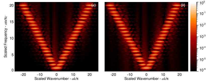
Figure 1: Spectra of waves obtained for the simple 1-D analog model of meridional circulation. Spectra of the waveform (16) are shown as a function of a dimensionless frequency $a\omega/\pi c$ and wavenumber $ak/\pi$. The scaling is such that power from the mode with degree $l$ is concentrated near the points $(\pm l,l)$. ($a$) The power spectrum in the absence of flow. ($b$) The power spectrum resulting from a flow with a maximum value of the Mach number $U_{0}/c=10^{-1}$ (chosen to be large for illustrative purposes). The meridional flow varies spatially as the fundamental sinusoid (15) that vanishes at both ends. The flow distorts the wavenumber sidelobes arising from spatial windowing. For both spectra, the damping rate is given by $\eta_{l}=2.5\times 10^{-2}\Delta\omega$, where $\Delta\omega=\pi c/a$ is the frequency spacing between modes. For a sound speed appropriate for the middle of the solar convection zone ($c\approx 0.1$ Mm s^-1) and a domain length of half the circumference of the Sun at that depth ($a=600\pi$ Mm), this damping rate is equivalent to a linewidth $\Gamma=\eta_{l}/\pi=1.3\mu$Hz.

where $\theta_{l}$ is a random phase with uniform distribution and ${\cal A}_{l}$ is the rms average over $j$ of the amplitudes $A_{lj}$. Figure 1 displays the power spectrum that results from applying a cosine window function and taking the spatial Fourier transform of Equation (16) with $U_{0}$ chosen such that $M=U_{0}/c=0.1$. While this value is unrealistically large for meridional flows in the Sun, it was selected here purely for clarity of illustration. The spatial Fourier transform of a function $f(x)$ is defined as follows:

$$\tilde{f}(k)=\int_{-\infty}^{\infty}f(x)\,{\rm e}^{-{\rm i}kx}\;{\rm d}x,$$ (17)

such that positive $k$ corresponds to waves propagating in the positive $x$-direction.

The power in each normal mode is confined in a narrow frequency band about $\omega=\omega_{l}$, and is further concentrated in wavenumber bands into two separate branches, a positive-$k$ branch and negative-$k$ branch. These branches arise from the decomposition of the normal mode into waves propagating in opposite directions. The power in one branch is not necessarily symmetric with the other branch, since the modes are capable of interfering with each other because of their finite lifetimes. If the damping rates become sufficiently small compared to the frequency spacing between modes ($\eta_{l}\ll\pi c/a$), this interference effect disappears. For all illustrations appearing in this paper we have chosen a damping rate such that the ratio of the damping rate to the frequency spacing is roughly 10 times larger than the actual value for low-degree $p$ modes, but comparable to that for modes of intermediate degree. The chosen value ($\eta_{l}/\Delta\omega=2.5\times 10^{-2}$) produces mode interference with a small but noticeable effect.

Each mode appears with a series of spatial sidelobes. The amount of power in each sidelobe is a complicated function of the spatial windowing and the deviation of the eigenfunction from its zero-order (unperturbed by $U$) sinusoidal form. To generate the power spectra, we applied a cosine window function to reduce the spread of power due to windowing. Had we failed to apodize, the spread would have been worse; a Fourier transform over a finite domain effectively has a top-hat window function which spreads power rather broadly, due to its jump discontinuities. In power spectra of solar oscillations, similar spatial windowing effects (often called spatial leaks) arise automatically from a variety of sources, including the reduced spatial resolution at the poles, the lack of sensitivity to motions transverse to the line of sight, and the visibility of only one side of the Sun at any instant.

3.3 Granulation Noise

The Sun’s meridional flow does not produce a Doppler shift as extreme as that illustrated in Figure 1, as the Mach number of the flow is likely to be inordinately small, perhaps on the order of $10^{-4}$ or $10^{-5}$. Whether such a small signal can be extracted from the observations depends on the level of the noise. Therefore, in order to assess the detectability of a particular meridional flow, we must include noise. For instruments such as MDI on SOHO and HMI on the soon-to-be-launched SDO that use a photospheric line, the primary source of noise is solar granulation. Owing to the relatively short lifetime and small spatial scale of solar granulation, the noise spectrum generated by granulation is broad both in frequency and wavenumber. Thus, in our 1-D analog, we add white Gaussian noise, $N(x,\omega)$, to the wave field with a specified rms amplitude:

$$\tilde{v}(x,\omega)=N(x,\omega)+J^{1/2}\sum_{l=1}^{\infty}{\cal A}_{l}\,{\rm e}^{{\rm i}\theta_{l}}\,Q_{l}(x,\omega).$$ (18)

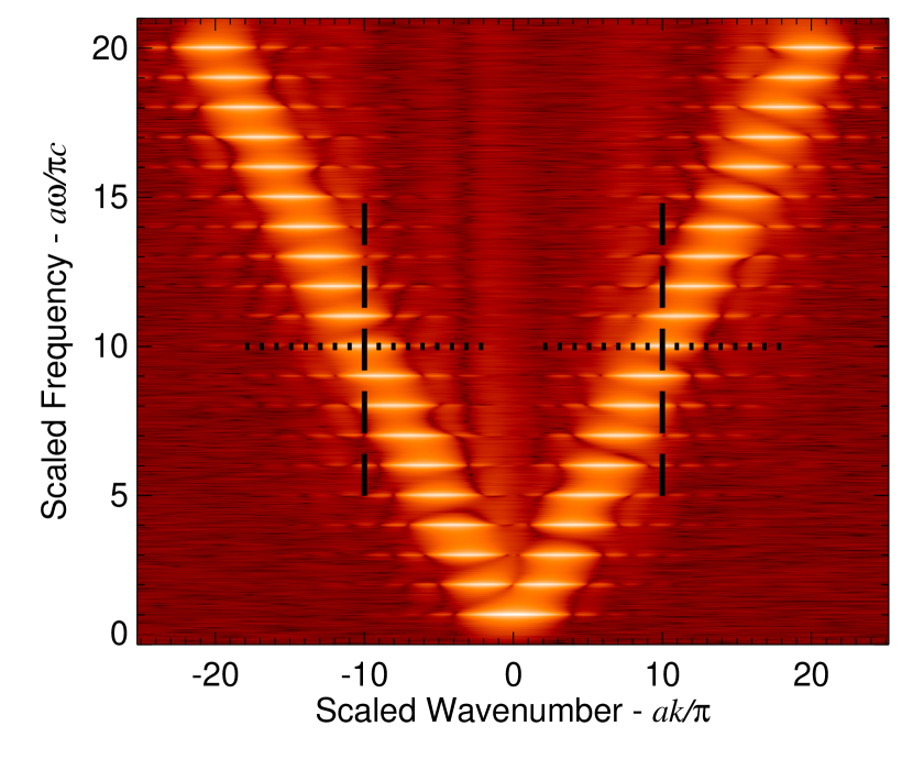
Figure 2: Same as Figure 1$b$, except that the maximum Mach number is $10^{-3}$ and white Gaussian noise has been added. The ratio of signal to noise is appropriate for low-degree $p$ modes and has been estimated from observations from a variety of sources (see §3.3). The Doppler shift is difficult to see by eye for such a low Mach number, and the spatial sidelobes, so prominent in Figure 1, have been partially obscured. The dashed lines mark the cuts at constant wavenumber $ak/\pi=\pm l$ shown in Figure 3$a$, the dotted lines the cuts at constant frequency $a\omega/\pi c=l$ shown in 3$b$.

The actual noise level for the MDI instrument is difficult to estimate because the power that appears between the $p$-mode peaks is largely the contribution of the overlapping wings of a large number of modes (personal communication, J. Schou, August 2009). Since a direct measurement of the level of noise for MDI is unavailable, we have attempted to estimate the noise by scaling observations obtained with other instruments for which a careful calibration of noise and signal has been obtained. Our estimate is based on the level of noise measured in a 496-day data set from the GOLF instrument (Fletcher et al., 2009). This level is scaled to that pertaining to an equivalent data set spanning 60 days, obtained from longitudinally averaged medium-$l$ MDI data with 130 latitudinal pixels. Further, we have assumed that 10-years worth of independent 60-day observations have been averaged together to reduce the noise. The resulting signal-to-noise ratio is roughly 50. A similar estimate can be obtained by evaluating at 3 mHz the spectral power distribution of granular power modeled by Harvey et al. (1993) with a granular growth timescale of 220 s and rms velocity of 0.6 km s^-1 (Keil, 1980). The mode amplitudes were estimated from measurements of the peak, spectral power density for low-degree modes obtained by BiSON (Chaplin et al., 2005). The scaling follows Christensen-Dalsgaard & Gough (1982) and takes into account that the BiSON spectral line (K $\lambda 769$ nm) is formed in the chromosphere and that the MDI spectral line (Ni I $\lambda 676.8$ nm) is photospheric. Figure 2 shows the power spectrum that results when such noise is present for a flow with a smaller Mach number: $U_{0}/c=10^{-3}$. The Doppler shift is now too small to be seen by eye, and the spatial sidelobes have diminished in prominence.

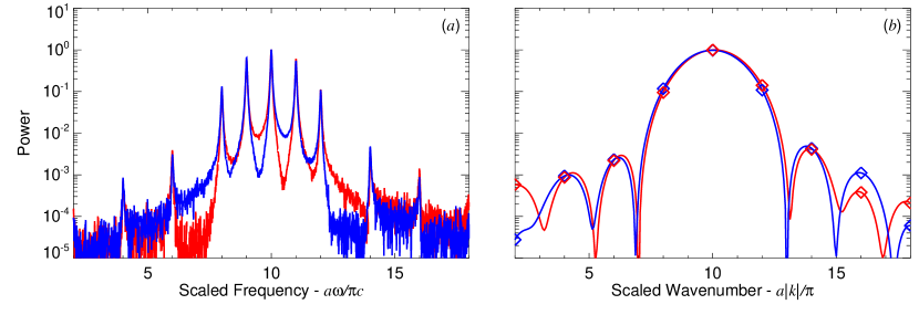
Figure 3: Cuts through the spectrum shown in Figure 2 at ($a$) constant wavenumber $ak/\pi=\pm l$ and ($b$) constant frequency $a\omega/\pi c=l$ for $l=10$. The blue and red curves correspond to waves propagating in the positive and negative $x$-direction—the right (prograde) and left (retrograde) branches in Figure (2) respectively. The Doppler effect manifests as a clear shift of the power distribution in the wavenumber, but not in frequency. In panel ($a$), the spatial sidelobes from modes with nearby $l$ generate a comb of frequencies that do not shift when a meridional circulation is present. The amplitude of each individual peak depends on the spatial windowing, the lifetime of the mode, and weakly on the flow speed and profile. In panel ($b$), the peaks are the spatial leaks generated by the $l=10$ mode, shifted slightly by the background flow.

As mentioned previously, for normal modes, the Doppler shift acts on the local wavenumber $k$ instead of acting on the mode frequency $\omega$, thus causing a shift in the sidelobe pattern. This is clearly visible in Figure 1$b$. The prograde branch ($k>0$) possesses a steeper slope than the retrograde branch ($k<0$). Yet the mode power within each branch is centered around the same frequency. Note that any attempt to measure a frequency shift by fitting a smooth profile $F(\omega)$ (such as a Lorentzian) at fixed $k$ will be frustrated by the fact that the power is confined to discrete frequencies that are unshifted (to first order in the Mach number) by the velocity feld. This is illustrated further in Figure 3, where we present two pairs of cuts through the power spectrum, one pair at constant wavenumber, and the other at constant frequency. Each pair is composed of a cut through the retrograde branch and a separate cut through the prograde branch. The locations of these cuts are indicated in Figure 2. The retrograde and prograde branches are shown in red and blue, respectively, in Figure 3.

Figure 3$a$ depicts cuts through the spectrum as a function of frequency for the constant value of the wavenumber $k$ corresponding to $l=10$ ($k=10\pi/a$). Rising up above the noise we see not only the mode frequency associated with that value of $l$, but also all the frequencies of the modes with nearby values of $l$ (due to their spatial sidelobes and finite lifetime). This comb of frequencies has an envelope which is modulated by the flow velocity, because both the principal peak and the windowing sidelobes are modified by the Doppler effect. The envelope is by no means Lorentzian, nor is it symmetric. Its exact shape is a complicated function of the flow velocity $U(x)$, the spatial window function, and the amplitudes and phases of the nearby modes. The Doppler effect is more evident in cuts through the power spectrum at constant frequency, illustrated in Figure 3$b$. There is a small but clear systematic shift between the two curves which is produced by the presence of the flow. The signature of the noise appears to be much less prominent in Figure 3$b$ than in Figure 3$a$. This is an illusion arising from the limited spectral resolution in Figure 3$b$. The curves appear smoother simply because the noise (and signal) exist only in the finite domain $x\in[0,a]$; therefore, the $k$-resolution $\delta k$ in the power spectrum is broad relative to the scale of the plot: $\delta k\approx 2\pi/a$ (or 2 in the dimensionless units employed in the figure). If a discrete Fourier transform were employed instead, only every other tick mark would be sampled, as is indicated by the diamonds in Figure 3$b$. The noise’s influence manifests predominantly as the growing disagreement between the power in the sidelobes with increasing distance from the central peak.

4 Measuring the Meridional Flow through Variations in the Spatial Phase

Since power in the spatial sidelobes is modified by a meridional flow, one might attempt to measure the flow by a careful analysis of those sidelobes. Since the sidelobes are sensitive to a large number of well-known, but poorly determined, leakage effects (incomplete observational coverage of the solar surface, foreshortening, velocity projection onto the line of sight, camera imperfections, etc.), we cannot expect to measure the meridional flow from their absolute height. The only hope that persists is in attempting to measure the difference in power between the prograde and retrograde branches. However, due to the fact that the power in the sidelobes is several orders of magnitude lower than the central peak, such a measurement scheme is likely to be fraught with signal-to-noise problems, particularly since the effect of the meridional flow is expected to be rather weak anyway. Moreover, this scheme would also be complicated by the fact that the complete pattern of the sidelobe structure will not be available in finitely sampled data. (In Figure 3$b$, the diamond symbols indicate which wavenumbers would be represented by a discrete transform).

Because of these difficulties, we expect that a more promising means of measuring the meridional flow seismologically would involve exploitation of the wave phase instead of just its power. One needs to be careful here with the use of the word phase. Does one mean the phase of the spatial and temporal transform, i.e., the phase of the spectral component? Or does one mean the phase of the wave in configuration space? In the remainder of this section, we propose a technique which is a hybrid of these two options. To be explicit, the procedure derives the meridional flow from measuring the phase of the wave expressed as a function of the temporal frequency and of latitude.

4.1 Spatial Variation of the Phase

Examination of Equations (18) and (13) reveals that near a resonant frequency ($\left|\omega-\omega_{l}\right|\lesssim\eta_{l}$) the waveform simplifies greatly:

$$\tilde{v}(x,\omega_{l})\approx N(x,\omega_{l})+\frac{1}{2}J^{1/2}{\cal A}_{l}\,\eta_{l}^{-1}\,{\rm e}^{{\rm i}\theta_{l}}\,\sin(k_{l}x)\;\exp\left(-{\rm i}\frac{k_{l}}{c}\int_{0}^{x}U\,{\rm d}x^{\prime}\right).$$ (19)

In the absence of noise, the phase $\phi_{l}$ of the wave is therefore easily determined:

$$\phi(x,\omega_{l})\equiv\arg\left\{\tilde{v}(x,\omega_{l})\right\}\approx\theta_{l}-\frac{k_{l}}{c}\int_{0}^{x}U\,{\rm d}x^{\prime}.$$ (20)

From Equation (20) it should be noticed that the modulation of the phase, considered as a function of position $x$, has a relatively simple dependence on the flow speed. In fact, the derivative of the phase with respect to position depends only on the flow and several presumably known constants:

$$\frac{\partial\phi(x,\omega_{l})}{\partial x}=-\frac{\pi l}{ca}\,U(x).$$ (21)

Here we have utilized the quantization condition for the wavenumber, Equation (5), to obtain the dependence on the degree $l$.

Equation (21) suggests an analysis scheme to extract the meridional flow profile $U(x)$ from observations of the wave field. In the absence of noise, one could sample the temporal Fourier transform of the wave field at a resonant frequency $\omega=\omega_{l}$, compute the phase $\phi_{l}(x)$, differentiate with respect to $x$, and finally use Equation (21) to obtain the flow as a function of $x$ (the analog of latitude in our 1-D model). Of course, in real observations, noise will be an issue; however, the effects of noise can be reduced by averaging the Fourier transform of the wave field over a band of frequencies centered on a resonant frequency $\omega_{l}$ with a width of $2\eta_{l}$ to generate an “average mode eigenfunction” $\bar{v}_{l}(x)$. Since the phase of the noise is uncorrelated over this frequency band, whereas the phase of the mode is correlated, $\bar{v}_{l}(x)$ is less contaminated by noise than the wave signal at a single frequency. Thus, a better estimate of the phase $\phi_{l}(x)$—and the amplitude $V_{l}(x)$—of the waveform can be obtained through the following equations:

$$\bar{v}_{l}(x) \equiv \frac{1}{2\eta_{l}}\int_{\omega_{l}-\eta_{l}}^{\omega_{l}+\eta_{l}}\tilde{v}(x,\omega)\;{\rm d}\omega\,,$$ (22)

$$\phi_{l}(x) \equiv \arg\left\{\bar{v}_{l}(x)\right\}\,,$$ (23)

$$V_{l}(x) \equiv \left|\bar{v}_{l}(x)\right|\,.$$ (24)

Why the amplitude $V_{l}$ is important will become apparent in a moment.

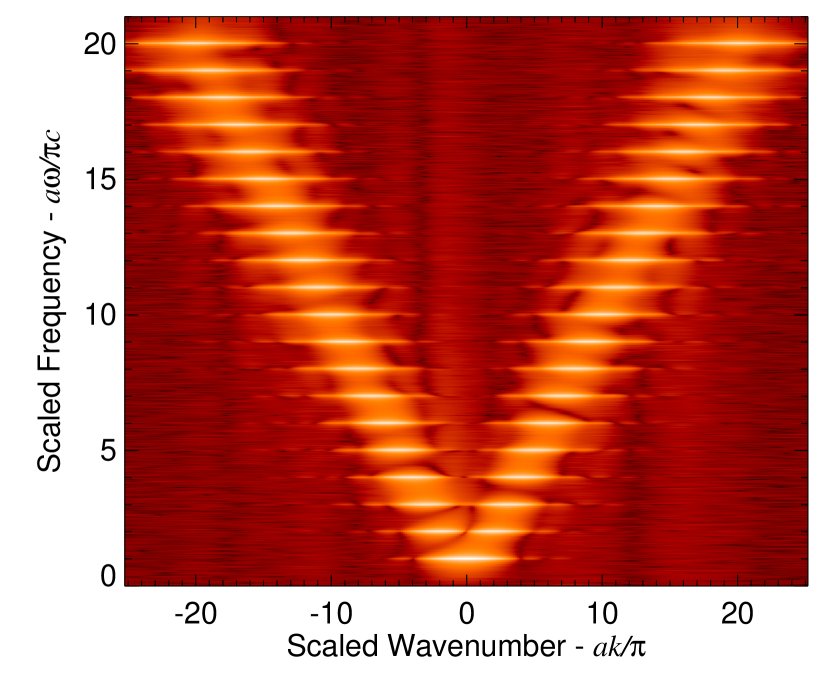
Figure 4: Power spectrum generated for a fast flow ($U_{0}/c=0.1$) with the cubic flow profile given by Equation (25). Since the flow profile is antisymmetric, instead of undergoing a Doppler shift, each branch is Doppler broadened. The broadening has caused partial merger of the spatial sidelobes.

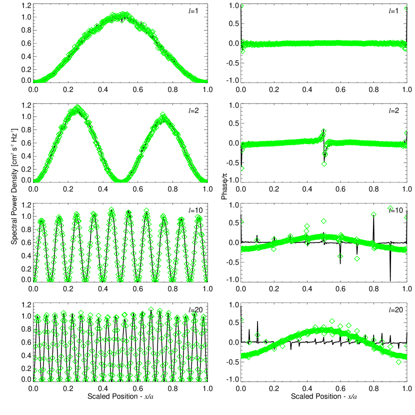
Figure 5: Spectral power density (left column) and phases (right column) of a subset of modes calculated using Equations (22)–(24) and the artificial data displayed in Figure 4. The origin of the phase is defined to be zero in the absence of noise and background flow $U$, and is determined by demanding that the spatial average of $\phi_{l}$ vanishes. The black curve shows the results in the absence of flow, and the green diamonds show the results when the flow field is present. The magnitude of the phase variation increases linearly with $l$, as expected from Equation (21).

The amplitude and phase defined in this fashion have been computed for a variety of model parameters. Figures 4 and 5 show the results for a flow profile that is antisymmetric about $x=a/2$,

$$U(x)=-12\sqrt{3}\;\,U_{0}\;a^{-3}\,x\,(x-a/2)\,(x-a).$$ (25)

This cubic form produces a flow speed that vanishes at both ends ($x=0$ and $x=a$) as well as in the middle $x=a/2$. The flow attains maximum and minimum values of $\pm U_{0}$, and for Figures 4 and 5 we have employed a large Mach number ($U_{0}/c=0.1$) for clarity of illustration. The flow is everywhere directed away from the center of the domain (i.e., the equator), much as the Sun’s meridional circulation is generally poleward in the outer layers of the convection zone. We have intentionally chosen a functional form that is non-sinudoidal to avoid using a flow that can be constructed from a finite number of mode eigenfunctions.

Figure 4 shows the power spectrum obtained for this flow profile. We point out that, unlike the previous example, the flow profile is antisymmetric, and therefore, the mode power in each branch is Doppler broadened instead of Doppler shifted. Figure 5 presents the square of the amplitude $V_{l}^{2}$ and the phase $\phi_{l}$, both calculated from the same wave field for a selection of modes. The square of the amplitude is scaled such that it would have unit maximum in the absence of both the noise and the flow $U$. The phase is measured relative to the average phase obtained by integrating the phase over the entire $x$-domain. The noise is clearly evident in both the amplitudes and the phases. Furthermore, the phase is poorly determined wherever the amplitude is small. Thus, locations of poor phase determination appear more frequently for higher-degree modes. The lack of uniformity in the height of the amplitude peaks arises from both the noise and the interference with nearby modes. We note further that the magnitude of the maximum phase grows linearly with $l$, as is predicted by Equation (21).

The linear dependence on $l$ suggests a simple scheme to reduce the influence of the noise further. An obvious procedure is to average $\phi_{l}$ over modes. But instead, we average $\phi_{l}/l$ in order to remove the leading behavior on mode degree. Thus, we define a mean phase function $\Phi(x)$ according to:

$$\Phi(x)\equiv\sum_{l}w_{l}(x)\;\phi_{l}(x)/l,$$ (26)

for a set of weighting functions $w_{l}(x)$. The fact that the phase becomes poorly determined when the amplitude $V_{l}(x)$ is small suggests that a weighting based on the computed amplitudes would be effective. Since the amplitudes defined by Equation (24) are non-negative, we choose to weight linearly with $V_{l}$:

$$w_{l}(x)=\frac{V_{l}(x)}{\sum_{l}V_{l}(x)}.$$ (27)

From the phase function $\Phi(x)$ one can derive the flow velocity by differentiation:

$$c^{-1}U(x)\approx-\frac{a}{\pi}\frac{{\rm d}\Phi}{{\rm d}x}.$$ (28)

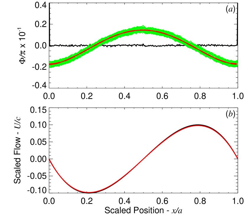
Figure 6: The mean phase function $\Phi(x)$ and the meridional flow profile derived from the phase function. The flow possesses an antisymmetric, cubic profile with a maximum Mach number of $U_{0}/c=10^{-1}$. ($a$) The mean phase function $\Phi$ as a function of position $x$. The black curve shows the phase function in the absence of flow, while the green diamonds (appearing as a blurred band solely because of the high density of points) show the result in the presence of the flow. The solid red curve is a low-degree polynomial fit to the phase function. The errors in the fit are exceedingly small, and thus, even though dashed red curves have been included to mark $3\sigma$ errors, the error curves are indistinguishable from the fit itself. ($b$) The input flow field, defined by Equation (25), is indicated by the black curve. The flow field derived by differentiating the red curve in panel $a$ is shown in red (lying nearly on top of the black curve). For the fast flow considered here, the phase-extraction technique recovers the input velocity remarkably well.

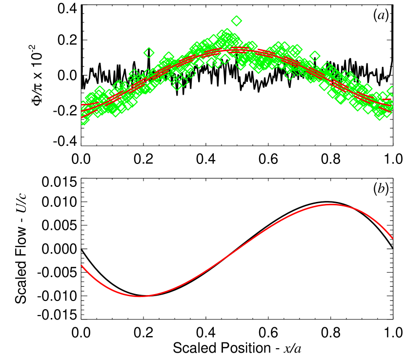
Figure 7: Same as Figure 6 except that the maximum Mach number is smaller: $U_{0}/c=10^{-2}$. In panel ($a$) the dashed red curves mark $\pm 3\sigma$ errors in the fitted quantity.

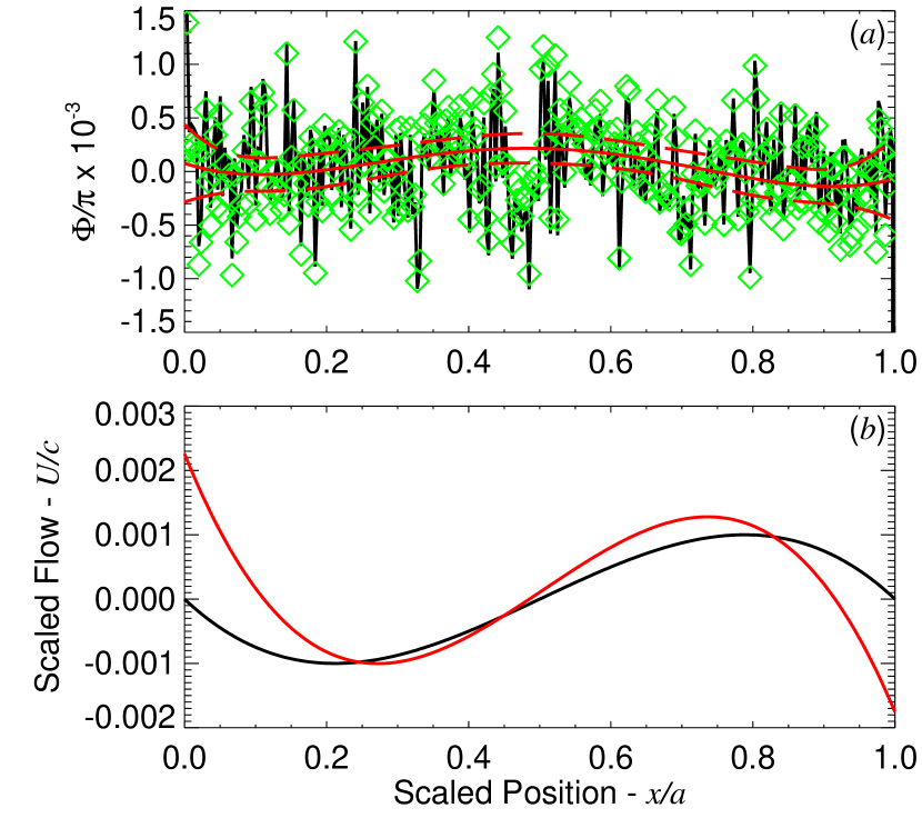
Figure 8: Same as Figure 6 except that $U_{0}/c=10^{-3}$. The phase extraction procedure works well in the interior, but has begun to fail at the edges of the domain where all the eigenfunctions have nodes.

The results of this procedure are illustrated in Figures 6–8, which display the mean phase function $\Phi(x)$ and the derived flow profile $U(x)$. The averaging has been perfomed over all modes with $l\leq 20$. Each figure corresponds to a different maximum flow speed $U_{0}/c$, ranging from $10^{-1}$ to $10^{-3}$. The upper panels show the mean phase functions and low-degree polynomial fits to the same. The lower panels show the derived flow profiles obtained by differentiating the polynomial fit to the mean phase function. For large Mach numbers ($M\gtrsim 10^{-2}$) the flow profile is recovered with great fidelity over the entire spatial domain. As the Mach number decreases, the recovered flow profile begins to diverge from the input flow profile, although initially only near the edges of the domain. This property is to be expected: the edges of the domain are zeros of the eigenfunctions for all degrees $l$, and, therefore, the determination of the phase $\phi_{l}$ is poor there for all modes. As the Mach number falls further ($M\lesssim 10^{-4}$), the noise comes to dominate and the recovered flow profile bears little resemblance to the input values.

5 Discussion

The principles we have illustrated with our 1-D model can be applied to the Sun. The most significant difference is that, for each mode, $c^{-1}U$ in Equation (28) should be replaced by its appropriately weighted vertical average $\left<c^{-1}U_{ln}\right>$. For deeply penetrating modes, the high-order asymptotic approximation to the oscillation eigenfunctions provides an adequate first guide (Gough, 1993), yielding a weighting function $W(r,\omega/L)$ that changes form at the lower turning point $r_{\rm t}$ given implicitly by $c(r_{\rm t})/r_{\rm t}=\omega/L$ where $L=l+1/2$. Below the lower turning point the weighting function vanishes, $W=0$, and above the lower turning point it is given by

$$W\left(r,\frac{\omega}{L}\right)\sim\left(1-\frac{L^{2}c^{2}}{\omega^{2}r^{2}}\right)^{-1/2}.$$ (29)

Approximate weighting functions for higher-order modes are displayed by Gough & Toomre (1983).

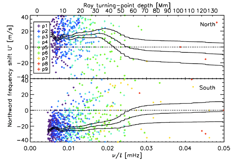
Figure 9: The observed frequency shift deduced from 3 months of MDI data obtained in 1997. The Doppler shift was measured by cross-correlating the two power spectra obtained by projecting separately onto northward- and southward-propagating waveforms. The apparent vanishing of the frequency shift for waves with a lower turning point greater than 40 Mm may be an artifact caused by the transition in the spectra from continuous ridges to discrete, normal mode peaks (after Mitra-Kraev & Thompson, 2007).

The analogous quantity to the return travel time in the one-dimensional model, $2a/c$, is the circumundulation time $T_{ln}\sim 4l\pi/\omega_{ln}$, the time an acoustic-wave packet takes to traverse a great circle around the Sun. If the damping time is short compared with the circumundulation time, $\eta_{ln}T_{ln}\gg 1$ (as is true for high-degree modes), the wave suffers little self interference, the mode power blends with nearby modes forming a continuous ridge, and measuring the apparent frequency shift $\delta\omega$ at given $l$ works well. But once $\eta_{ln}T_{ln}\ll 1$ (low-degree modes), resonances dominate the wave field, and the modes are well separated in the power spectrum, each with a frequency that is unshifted by the meridional circulation. Attempting to measure a shift by fitting a Lorentzian to the frequency profile, or cross-correlating the power from poleward- and equatorward-propagating waves, cannot therefore result in a meaningful nonzero value. Instead, a background flow shifts and broadens the distribution of power in degree $l$. As our discussion indicates, one expects a null frequency shift for waves of low $l$: once $\eta_{ln}T_{ln}\lesssim 1$, the apparent shift $\delta\omega$ must decline with decreasing $l$. Indeed that is just what appears to have been observed (Braun & Fan, 1998; Mitra-Kraev & Thompson, 2007), as is illustrated in Figure 9.

Misinterpreting this decline as a true decline in frequency has led to an erroneous inference about the depth of the reversal of the Sun’s meridional circulation. The circulation is well known to be directed poleward near the surface, and if the radial average $\left<c^{-1}U_{ln}\right>$ over most of the convection zone (as sampled by low-$l$ modes) vanishes, then the poleward surface flow must be counterbalanced by a deep equatorward flow within the convection zone. If $\delta\omega$ were a measure of that radial average, the flow reversal would be located at the lower turning point of the modes near where $\delta\omega$ starts to decline with decreasing $l$. That is just where the continuous ridges in the power spectrum of the modes give way to distinguishable discrete peaks. The transition occurs at $\nu/l\lesssim 20\mu$Hz (see Figure 9) which Mitra-Kraev & Thompson (2007) acknowledge corresponds to a turning point at about 40 Mm beneath photosphere. However, we have argued that this depth has actually little, if anything, to do with the location of the reversal of the real flow.

Since the eigenfrequencies are insensitive to the meridional flow, the only unambiguous way to detect meridional flow in the lower half of the convection zone is via the structure of the oscillation eigenfunctions. One telling property of that structure is that separability in space and time is destroyed by the flow, causing latitudinal variation in temporal phase. We propose here that the structure of the flow can in principle be determined from direct measurements of that phase. We recognize that the phase variation can equivalently be interpreted as a spatial variation at fixed time, which together with an accompanying amplitude variation, distorts the eigenfunction from its flow-free, spherical-harmonic counterpart. In a decomposition into spherical harmonics, this distortion appears as a leakage of power across degree $l$, that could conceivably be measured. However, we suspect that any attempt to measure that distortion directly is likely to be much more susceptible to noise; it would also need to be separated from the much larger contributions to the total distortion resulting from shear in the zonal flow.

Finally, it behooves us to address the likelihood that a reversal in the flow direction with depth will actually be detectable. Our simulations with 20 modes indicates that, if our error estimates are realistic, the lower limit on the Mach number for a measurable flow is between $10^{-4}$ and $10^{-3}$. That corresponds to a flow velocity between about 20 and 200 m s^-1 at a depth of about 150 Mm. The lower value is comparable with the flow speeds in the convection-zone simulations by Miesch et al. (2008). So perhaps the detection of the flow reversal in the Sun is almost in sight.

References

- Basu & Antia (2003) Basu, S., & Antia, H. M. 2003, ApJ, 585, 553
- Braun & Fan (1998) Braun, D. C., & Fan, Y. 1998, ApJ, 508, L105
- Brun & Toomre (2002) Brun, A. S., & Toomre, J. 2002, ApJ, 570, 865
- Brun et al. (2004) Brun, A. S., Miesch, M. S., & Toomre, J. 2004, ApJ, 614, 1073
- Chaplin et al. (2005) Chaplin, W. J., Houdek, G., Elsworth, Y., Gough, D. O., Isaak, G. R., & New, R. 2005, MNRAS, 360, 859
- Christensen-Dalsgaard & Gough (1982) Christensen-Dalsgaard, J. C., & Gough, D. O. 1982, MNRAS, 198, 141
- Charbonneau (2005) Charbonneau, P. 20005, Living Rev. Sol. Phys., 2, 2
- Dikpati & Gilman (2006) Dikpati, M., & Gilman, P. A. 2006, ApJ, 649, 498
- Duvall & Hanasoge (2003) Duvall, T. L., Jr., & Hanasoge, S. M. 2009, ArXiv e-prints, 0905.3132
- Duvall (2003) Duvall, T. L., Jr. 2003, , in Proc. of SOHO 12 / GONG+ 2002, Local and Global Helioseismology: The Present and Future, ed. H. Sawaya-Lacoste, (ESA SP-517; Noordkwijk: ESA), 15
- Fletcher et al. (2009) Fletcher, S. T., Chaplin, W. J., Elsworth, Y., & New, R. 2009, ApJ, 694, 144
- Giles et al. (1997) Giles, P. M., Duvall, T. L., Jr., Scherrer, P. H., & Bogart, R. S. 1997, Nature, 390, 52
- Giles (2000) Giles, P. 2000, PhD Thesis (Stanford University)
- González Hernández et al. (2008) González Hernández, I., Kholikov, S., Hill, F., Howe, R., & Komm R. 2008, Sol. Phys., 252, 235
- Gough & Toomre (1983) Gough, D. O., & Toomre, J. 1983, Sol. Phys., 82, 401
- Gough (1993) Gough, D. O. 1993, in Proc. of Astrophysical fluid dynamics - Les Houches 1987, eds. J-P. Zahn and J. Zinn-Justin, (Elsevier), 399
- Haber et al. (2002) Haber, D. A., Hindman, B. W., Toomre, J., Bogart, R. S., & Larsen, R. M. 2002, ApJ, 570, 855
- Harvey et al. (1993) Harvey, J. W., Duvall, T. L., Jr., Jefferies, S. M., & Pomerantz, M. A. 1993, in Proc. of GONG 1992, Seismic Investigation of the Sun and Stars, ed. T. M. Brown, (ASPC #42: ASP), 111
- Hathaway et al. (1996) Hathaway, D. H., et al.1996, Science, 272, 1306
- Hindman et al. (2009) Hindman, B. W., Haber, D. A., & Toomre, J. 2009, ApJ, in press
- Keil (1980) Keil, S. L. 1980, ApJ, 237, 1035
- Komm et al. (1993) Komm, R. W., Howard, R. F., & Harvey, J. W. 1993, Sol. Phys., 147, 207
- Krieger et al. (2007) Krieger, L., Roth, M., & von der Lühe, O. 2007, Astronomishe Nachtrichten, 328, 252
- LaBonte & Howard (1982) LaBonte, B. J., & Howard, R. 1982, Sol. Phys., 80, 361
- Miesch et al. (2008) Miesch, M. S., Brun, A. S., DeRosa, M., & Toomre, J. 2008, ApJ, 673, 557
- Mitra-Kraev & Thompson (2007) Mitra-Kraev, U. & Thompson, M. J. 2007, Astronomische Nachtrichten, 328, 1009
- Rempel (2006a) Rempel, M. 2006a, ApJ, 647, 662
- Rempel (2006b) Rempel, M. 2006b, ApJ, 637, 1135
- Roth & Stix (2008) Roth, M. & Stix, M. 2008, Sol. Phys., 251, 77
- Švanda et al. (2007) Švanda, M., Kosovichev, A. G., & Zhao, J. 2007, ApJ, 670, L69
- Zhao & Kosovichev (2004) Zhao, J. & Kosovichev, A. G. 2004, ApJ, 603, 776