Simple isotherm equations to fit type I adsorption data

Abstract

A simple model to fit experimental data of adsorption of gases and vapours on microporous adsorbents (type I isotherms) is proposed. The main assumption is that the adsorbate phase can be divided into identical and non-interacting effective subsystems. This gives rise to a simple multiparametric isotherm based on the grand canonical ensemble statistics, whose functional form is a ratio of two polynomial functions. The parameters are interpreted as effective equilibrium constants. A simplified isotherm that reduces the number of adjustable parameters with respect to the general isotherm is also proposed. We show how to use these isotherms to fit the adsorption data in such way that the parameters have statistical significance. Due to their high accuracy, both isotherms can be used to estimate thermodynamic properties like isosteric and differential heats of adsorption. A simple method is presented for systems that show an apparent variation in the coverage limit with temperature. This method avoids overparametrization and improves fitting deviations. Finally, several applications to fitting data, taken from the literature, of adsorption of some gases on activated carbon, molecular sieving carbon, silica gel, and pillared clays are presented.

1 Introduction

Correlating adsorption data obtained from experiments or computer calculations is necessary to save time and efforts in additional experimentation or computing time. Because of the complexity of the equilibrium adsorption phenomenon, the research of new models of adsorption is still very active. A good parameter-adjustable model must fit well the experimental data and predict thermodynamic quantities correctly; therefore, it is necessary to analyse the model and assess its capabilities. Many industrial applications of adsorption encompass a wide range of adsorbent saturation. Thus, models which offer the experimentalist and process engineer the possibility to set the number of adjustable parameters are required.

Many adsorbents used in industry and research present certain degree of heterogeneity in terms of pore size distribution and surface topography. Depending on each of these factors, different isotherm models are proposed. For example, lattice gas theories which simplify the structure of the adsorbent surface by taking into account only the most important adsorption sites of the adsorbent surface or adsorption pores have been developed. Many of these theories are consistent with experiments and computer simulations [2, 39, 24, 16, 25, 1, 27, 28, 29, 30, 23]. A disadvantage of this kind of models is that many gas-solid systems present unique characteristics. Thus, they may not be applicable if some assumptions or conditions are violated.

Another commonly used method to obtain isotherms for heterogeneous systems is the integration over a patchwise topography of adsorption sites [10]. Modified isotherms arise by assuming an adsorption energy distribution function and an ideal local isotherm like the Langmuir equations. Even though some of these equations work well for a large number of systems, they present limitations associated with the assumptions of the particular model, e.g., some models do not provide the correct Henry’s law limit. Moreover, this integration method is somewhat difficult because the complexity of the adsorption energy distribution makes it difficult to obtain the analytical expression for the transformed isotherm. The equations of Sips [35], Toth [40], and UNILAN [36] are the most widely used isotherms of this type.

In this work simplified isotherms to fit type I adsorption data are proposed. The model to derive the isotherms is the cell model of adsorption shown by Hill [12, 14, 13], which is based on the grand canonical ensemble statistics. The general isotherm that arises from the cell model has been quite successful to fit experimental data of adsorption of gases on zeolites [31, 32, 3, 7, 8, 38, 33]. Recently, we showed how to employ this model to fit isotherms of adsorption of gases and vapours on zeolites [22] and that the parameters could be interpreted as adsorption equilibrium constants. Further validation of this generalized statistical thermodynamical adsorption (GSTA) model has been shown with excellent results for both adsorption data and thermodynamic properties [21, 20]. Here, we present an accurate extension of the GSTA model and a new simplified isotherm is derived from it. It is shown that these isotherm equations can be used to fit type I experimental adsorption isotherms and predict thermodynamic properties. To illustrate this idea, several experimental adsorption isotherms are correctly fitted with these isotherms. Furthermore, extrapolations to temperatures beyond the experimental temperature range are possible. Because of the complexity of heterogeneous adsorbents, it is suggested that the method presented here is semi-empirical and the cells ensemble can be considered as an effective grand ensemble of small subsystems.

2 Theory

2.1 The general adsorption isotherm

Consider a single-component gas in equilibrium with an adsorbate phase and suppose that the adsorbate phase can be divided into $M$ identical cells that are not interacting in the ensemble picture. This means that they are coupled by a very small interaction such that the exchange of molecules in between cells takes place in a time scale which is large in comparison with the characteristic time scales of the fundamental molecular processes that occur inside each cell. The total number of cells is temperature-independent and the cell volume as well. It is plausible to assume that a maximum of $n_{\mathrm{s}}$ molecules can adsorb on the subsystem, i.e. the adsorbent has a saturation limit. Under these assumptions we can express the grand canonical partition function $\Xi$ as a product of subsystem’s partition functions [14]:

$$\Xi=\xi^{M}$$ (1)

where

$$\xi=\displaystyle 1+\sum_{j=1}^{n_{\mathrm{s}}}K_{j}a^{j}$$ (2)

and $a$ is the activity of the system:

$$a=\frac{f}{P^{0}}$$ (3)

Since we are concerned with the low pressure regime then $a=P/P^{0}$. The equilibrium constant $K_{j}$ is expressed as

$$K_{j}(T)=\exp\Big{(}\frac{j\mu^{0}_{\mathrm{g}}-A_{j}^{\mathrm{S}}}{k_{\mathrm{B}}T}\Big{)}$$ (4)

where $\mu^{0}$ is the chemical potential of the gas at the reference pressure $P^{0}$ and $A_{j}^{\mathrm{S}}$ is a microscopic free energy which can be written in terms of the partition function of the subsystem with $j$ molecules and volume $v_{S}$ ($Q_{S}(T,v_{S},j)$):

$$A_{j}^{\mathrm{S}}=-k_{B}T\ln Q_{S}(T,v_{S},j)$$ (5)

Now the saturation of the system ($q$) is simply:

$$q=\frac{q_{\mathrm{m}}}{n_{\mathrm{s}}}\frac{\displaystyle\sum_{j=1}^{n_{\mathrm{s}}}jK_{j}a^{j}}{\displaystyle 1+\sum_{j=1}^{n_{\mathrm{s}}}K_{j}a^{j}}$$ (6)

Based on its definition, the term $K_{j}$ can be regarded as an adsorption equilibrium constant [22]. Therefore, in analogy with chemical equilibrium constants, we can propose the following relation:

$$\ln K_{j}=\ln K_{j}^{\circ}-\frac{\Delta h_{j}}{RT}$$ (7)

where $\ln K_{j}^{\circ}$ and $\Delta h_{j}$ are the change of entropy and enthalpy, respectively. They are related with the adsorption of $j$ molecules onto a representative microscopic subsystem at the reference pressure $P^{0}$. In his seminal paper, the Eq. (6) was also derived by Langmuir [18] using chemical kinetics for the case in which a site can hold several molecules and the adsorbent is composed by non-interacting sites. In light of his proposal, the term $K_{j}$ is partitioned as follows:

$$K_{j}=\frac{1}{j!}\prod_{i=1}^{j}R_{i}$$ (8)

In a similar fashion, $R_{j}$ obeys the following relation:

$$R_{j}=R_{j}^{\circ}\exp\Big{(}\frac{-\Delta\overline{h}_{j}}{RT}\Big{)}$$ (9)

where

$$R_{j}^{\circ} = \frac{jK_{j}^{\circ}}{K_{j-1}^{\circ}}$$ (10)

$$\Delta\overline{h}_{j} = \Delta h_{j}-\Delta h_{j-1}$$ (11)

In order to fit an isotherm at constant temperature using Eq. (6), the adjustable parameters are $\{R_{j}\}$ instead of $\{K_{j}\}$. For the case in which several isotherms at different temperatures have been measured, the adjustable parameters are $\{\ln R_{j}^{\circ}\}$, $\{\Delta\overline{h}_{j}\}$, and $q_{\mathrm{m}}$. Hence, a total of $2n_{\mathrm{s}}+1$ parameters are required.

The present model suggests that $\xi\rightarrow\Xi$ as the subsystem volume is increased. Thus, in order to predict $q$ we should assume that the maximum number of molecules $n_{\mathrm{s}}$ and the volume $v_{S}$ are very large. However if we assume that each $R_{j}$ is an adjustable parameter, then this would give us a large number of adjustable parameters with poor statistical confidence [33]. A solution to this problem is to assume $n_{\mathrm{s}}$ as a small number of molecules that adsorb into a microscopic imaginary effective subsystem, and the parameters $\{R_{j}\}$ as representative parameters of the experimental adsorption isotherm. The characteristics of the adsorbate+adsorbent system like molecule-surface and molecule-molecule interactions are included effectively in these subsystems; probably by a modified intermolecular potential. This is ad hoc guess is a convenient picture that allows us to apply the cell model to complex zeolite and heterogeneous systems in general.

The probability that a subsystem with $j$ adsorbed molecules will be found is (assuming ideal gas phase):

$$p_{j}=\frac{K_{j}a^{j}}{\xi}$$ (12)

Eq. (6) can be written as:

$$\theta=\frac{1}{n_{\mathrm{s}}}\sum_{j=1}^{n_{\mathrm{s}}}jp_{j}=\frac{1}{n_{\mathrm{s}}}\sum_{j=1}^{n_{\mathrm{s}}}f_{j}$$ (13)

here, $\theta=q/q_{\mathrm{m}}$, and $f_{j}$ is a fraction of the $n_{s}$ molecules that are found in subsystems with $j$ molecules. At low pressures the leading term in Eq. (13) is $f_{1}$ (as stated by the Henry’s law), and, as the pressure increases, the leading is $f_{2}$, and so forth. Consequently, within certain pressure range, there is an $f_{j}$ term that significantly contributes to the fractional coverage. Therefore, each parameter $K_{j}$ can be associated with data taken in a certain range of the saturation $q$. So we infer that these parameters might have large uncertainties if there is not enough data in their corresponding intervals .

The general isotherm (Eq. (6)) and its simplifications have been useful to fit isotherms of adsorption of gases and vapours on zeolites at different temperatures, where the experimental isotherms show clearly a saturation limit, or are reported within the same range of saturation (see Refs. [31, 32, 3, 7, 8, 38, 22, 21, 20]). However, a great number of adsorption systems do not show this behaviour because experiments typically are performed along the same pressure range; therefore, the isotherms apparently show that the saturation limit depends on temperature (i.e., $q_{\mathrm{m}}$ tend to increase with a decrease in temperature). Now, consider certain isotherm at temperature $T_{1}$, if we consider that $n_{\mathrm{s}}=3$, then we have the following adjustable parameters: $K_{1},\,K_{2},\,K_{3}$, and $q_{\mathrm{m}}(T_{1})$. Also, suppose that we have a second isotherm at temperature $T_{2}$ and its apparent saturation limit is $q_{\mathrm{m}}(T_{2})$; if $T_{2}<T_{1}$, then $q_{\mathrm{m}}(T_{2})>q_{\mathrm{m}}(T_{1})$. This would suggest that, as the temperature decreases, new subsystems are created, but this would be an inconsistency for our model. To solve this problem, we introduce a new equilibrium parameter $K_{n_{\mathrm{s}}+1}$ that takes into account the adsorption of an extra molecule on the subsystem at high pressures and low temperatures. Because this new parameter describes the adsorption at these conditions, it is possible that there is not enough experimental data to estimate $\ln R_{n_{\mathrm{s}}+1}^{\circ}$ and $\Delta\overline{h}_{n_{\mathrm{s}}+1}$. To solve this problem we assume that $R_{n_{\mathrm{s}}+1}=R_{n_{\mathrm{s}}}$ and write

$$K_{n_{\mathrm{s}}+1}=\frac{R_{n_{\mathrm{s}}}}{n_{\mathrm{s}}+1}K_{n_{\mathrm{s}}}$$ (14)

Here we have assumed that the change of both entropy and enthalpy of adsorption of the $(n_{\mathrm{s}}+1)$th molecule on the microscopic cell is the same for the adsorption of the $n_{\mathrm{s}}$th molecule (i.e., $R\ln R_{n_{\mathrm{s}}+1}^{\circ}=R\ln R_{n_{\mathrm{s}}}^{\circ}$ and $\Delta\overline{h}_{n_{\mathrm{s}}+1}=\Delta\overline{h}_{n_{\mathrm{s}}}$). If we suppose this is applicable for $l$ extra molecules, then this result is generalized as follows:

$$K_{n_{\mathrm{s}}+l}=\frac{R_{n_{\mathrm{s}}}}{n_{\mathrm{s}}+l}K_{n_{\mathrm{s}}+l-1}$$ (15)

Now, $\xi$ becomes:

$$\xi=1+\sum_{j=1}^{n_{\mathrm{s}}+l}K_{j}a^{j}$$

and the isotherm is:

$$q=\frac{q_{\mathrm{m}}}{n_{\mathrm{s}}+l}\frac{\displaystyle\sum_{j=1}^{n_{\mathrm{s}}+l}jK_{j}a^{j}}{\displaystyle 1+\sum_{j=1}^{n_{\mathrm{s}}+l}K_{j}a^{j}}$$ (16)

This is our extension to the GSTA model and we will show in section 3 how to apply this Eq. to obtain statistically reliable estimation of the parameters.

2.2 A simplified adsorption isotherm

In order to reduce the number of adjustable parameters and improve the confidence intervals around the parameters’ estimates, suppose there is a reference temperature $T^{\circ}$ at which the molecules in the subsystem behave as a microgas. This microgas can be either two or three dimensional, it depends on the adsorbent characteristics. Hence we obtain:

$$K_{j}^{\circ}=\frac{(K^{\circ})^{j}}{j!}$$ (17)

Under these assumptions, it is obtained the adsorption isotherm:

$$q=\frac{q_{\mathrm{m}}}{n_{\mathrm{s}}+l}\frac{\displaystyle\sum_{j=1}^{n_{\mathrm{s}}+l}\frac{\displaystyle\exp(-\Delta h_{j}/RT)}{\displaystyle(j-1)!}(K^{\circ}a)^{j}}{\displaystyle 1+\sum_{j=1}^{n_{\mathrm{s}}+l}\frac{\displaystyle\exp(-\Delta h_{j}/RT)}{\displaystyle j!}(K^{\circ}a)^{j}}$$ (18)

comparing with Eq. (16) we have:

$$K_{j}=\frac{(K^{\circ})^{j}}{j!}\exp(-\Delta h_{j}/RT)\qquad j=1,\ldots,n_{\mathrm{s}}$$ (19)

From Eq. (15) we obtain:

$$K_{n_{\mathrm{s}}+l}=\frac{\displaystyle K^{\circ}\exp[-(\Delta h_{n_{\mathrm{s}}}-\Delta h_{n_{\mathrm{s}}-1})/RT]}{\displaystyle n_{\mathrm{s}}+l}K_{n_{\mathrm{s}}+l-1}$$ (20)

Here, the fitting parameters are $\{\Delta h_{j}\}$, $K^{\circ}$, and $q_{\mathrm{m}}$. Hence, we have reduced the number of parameters almost by half.

2.3 Isosteric heat of adsorption

From Eq. (4) we get

$$\Delta h_{j}=u_{j}-jh_{\mathrm{g}}^{0}$$ (21)

where $u_{j}$ and $h_{\mathrm{g}}^{0}$ are the energy of $j$ molecules in a subsystem and the molar enthalpy of the gas phase at $P^{0}$, respectively, and $\Delta h_{j}$ is the change of enthalpy related to the adsorption of $j$ molecules on a subsystem. In principle $\Delta h_{j}$ is temperature-dependent, but for the sake of simplicity, we have assumed that both $h_{\mathrm{g}}^{0}$ and $u_{j}$ are temperature-independent. The isosteric heat of adsorption can be calculated by means of the following formula [11]:

$$q^{\mathrm{st}}=h_{\mathrm{g}}-u_{\mathrm{a}}$$ (22)

where $h_{\mathrm{g}}$ and $u_{\mathrm{a}}$ are the molar enthalpy of the gas phase and adsorbate molar internal energy respectively. Define the following average for an arbitrary discrete real function $g_{j}$:

$$\langle g_{j}\rangle_{0}=\sum_{j}p_{j}g_{j}$$

It is easy to show that the isosteric heat of adsorption is a ratio of covariances:

$$-q^{\mathrm{st}}=\frac{\langle j\Delta h_{j}\rangle_{0}-n_{\mathrm{s}}\theta\langle\Delta h_{j}\rangle_{0}}{\langle j^{2}\rangle_{0}-n_{\mathrm{s}}^{2}\theta^{2}}$$ (23)

where $\theta=q/q_{\mathrm{m}}$. From the above Eq., the two following limits arise:

$$\lim_{\theta\rightarrow 0}q^{\mathrm{st}} = -\Delta\overline{h}_{1}$$ (24)

$$\lim_{\theta\rightarrow 1}q^{\mathrm{st}} = -\Delta\overline{h}_{n_{\mathrm{s}}}$$ (25)

This result establishes a physical interpretation to the first and the last enthalpies of molecular addition.

3 Results and discussion

The unweighted least-squares Levenberg-Marquardt algorithm was employed to fit the published experimental data used in this work. Details of the results of fitting Eqs. (18) and (16) to several experimental adsorption data are shown in Tables 1 and 2; the parameters are tabulated with their corresponding marginal confidence intervals [5, 34]. The study of these intervals is necessary to avoid over-interpretation of the parameters [17] and to estimate uncertainties in predicted thermodynamic properties. The parameter $\ln K^{\circ}$ (or $\ln K_{j}^{\circ}$) were used instead of $K^{\circ}$ (or $K_{j}^{\circ}$) due to the restriction $K^{\circ}>0$ (for all $j$). The following deviation parameter was employed to analyse the fittings accuracy:

$$D=\frac{100\%}{N_{\mathrm{T}}}\times\sum_{j=1}^{N_{\mathrm{temp}}}\sum_{i=1}^{N_{\mathrm{P}}(j)}\Bigg{|}\frac{q(P_{i},T_{j})-q_{\mathrm{exp}}(P_{i},T_{j})}{q_{\mathrm{exp}}(P_{i},T_{j})}\Bigg{|}$$ (26)

where $N_{\mathrm{temp}}$ is the number of isotherms, $N_{\mathrm{P}}(j)$ is the number of experimental data taken at $T_{j}$ temperature, $N_{\mathrm{T}}$ is the total number of experimental data, $q(P_{i},T_{j})$ is the calculated saturation, and $q_{\mathrm{exp}}(P_{i},T_{j})$ is the experimental saturation. It can be noticed in Table 1 that the deviation parameter ($D$) in all cases is less than $5\%$.

In Fig. 1 we fit the experimental isotherms of $\mathrm{SF_{6}}$ adsorption on pillared clay (designated as W-A(673)) measured by Bandosz et al. [4] with Eq. (18). It can be noticed a good agreement between the experimental data and Eq. (18). For this set of isotherms, the correction term (Eq. (20)) was used ($l=1$) and it was obtained a deviation of 2.97 %. If this correction were not applied ($l=0$) the deviation would be 5.2 %. Fig. 1 suggests that Eq. (18) is useful for isotherms with complex shapes like those reported in Ref. [4]. These experimental isotherms were also fitted using the 5-parameter Toth equation and it was obtained a deviation of 17.8%. On the other hand, Eq. (16) could be used to fit these experimental isotherms, but more parameters would be necessary and this would lead to large error bars and thermodynamic properties with larger uncertainties. Bandosz et al. [4] reported additional single-component experimental isotherms of propane and sulfur hexafluoride adsorption on various heat-treated pillared clays; a total of six adsorbate+adsorbent systems were studied. Given that the results are similar, here only two analysed systems are reported in Table 1. However, the deviation was within 1 and 3 % for the six adsorbate+adsorbent systems.

Fig. 2 shows the estimated isosteric heat of adsorption as a function of adsorbed volume and the corresponding marginal confidence intervals [5, 34] for the $\mathrm{SF_{6}}$+W-A(673) system. This Fig. shows that $q^{\mathrm{st}}$ is nearly constant around 25.5 kJ/mol. Bandosz et al. [4] used a virial isotherm [9, 15] to correlate their data. They obtained plots of $q^{\mathrm{st}}$ with some oscillations near zero saturation around 25 kJ/mol; this result does not agree with that obtained here by means of Eq. (23). These differences might be due to the method used by Bandosz et al. [4]. They fitted small subsets of 15 adsorption data by using the virial-type isotherm and four parameters to fit each subset. Although this method is appropriate to fit the saturation data, the error bars reported by them correspond to standard deviations in the calculated isosteric heats of adsorption. If 95 % marginal confidence intervals are used, the error bars at low coverage would be larger and the oscillations in the isosteric heat might be within such error bars.

To illustrate the dependence of the isosteric heat of adsorption in terms of temperature, plots of $q^{\mathrm{st}}$ vs $T$ at three different saturations are shown in Fig. 3. As expected, the isosteric heat of adsorption does not significantly change within the experimental range of temperatures; this is typically observed in both experiments and molecular simulations. In the case in which it is necessary to take into account the dependency of isosteric heat of adsorption on temperature, the well known thermochemical formula [26] to calculate chemical equilibrium constants could be used to estimate $\ln K_{j}$ as a function of temperature in Eq. (4); an empirical model for the heat capacity would be necessary.

The fitting of the experimental isotherms of adsorption of 1,1,1,2,3,3,3-heptafluoropropane (HFC-227ea) on activated carbon is shown in Fig. 4. As in the previous case, the fittings are very accurate; the correction term was not necessary ($l=0$). Due to the complex pore structure of activated carbon, it is difficult to consider a subsystem as any specific region of the real adsorbent, for this reason it is convenient to regard each cell as an effective subsystem. The isosteric heat of adsorption calculated by using both Eq. (23) and the Toth equation are shown in Fig. 5. It can be noticed that both curves fairly agree. The differences are attributed to the fact that Yun et al. [42] only used two isotherms to calculate the isosteric heat of adsorption. They employed the parameters of each isotherm and the Clausius-Clapeyron equation to obtain the $q^{\mathrm{st}}$ vs $q$ plot. In contrast, here the complete set of experimental isotherms was used. A problem with the method of Yun et al. [42] is that the isosteric heat of adsorption is influenced by uncertainties in the adsorption data, and hence, very reliable isotherms are necessary to determine $q^{\mathrm{st}}$ if only two isotherms are to be employed.

The adsorption isotherms of $\mathrm{CO_{2}}$ on zeocarbon [19] and the fractions of molecules distributed among cells at 273.15 K and 313.15 K are shown in Fig. 6. The zeocarbon synthesized by Lee et al. [19] is a zeolite X/activated carbon mixture composed by 38.5 mass % zeolite X, 35 mass % activated carbon, 10 mass % inert silica, and 16.5 mass % zeolite A and P. For this system, Eq. (18) accurately fits the experimental data ($D=3.8\%$), and the correction term ($l=1$) in this case reduces the deviation by 2 % with respect to the $l=0$ case. The deviation is less than that obtained by using the Toth equation; which is one of the most used equations to fit these kind of adsorption data. Since the zeocarbon is a zeolite/activated carbon composite, that the adsorbate phase may be divided into identical weakly-interacting effective subsystems is again a suitable assumption for fitting and correlation purposes.

As it was mentioned in the previous section, at low pressures the leading term is $f_{1}$ and each $f_{j}$ significantly contributes within a certain region of the isotherm. It can be noticed in Fig. 6a that the saturation ($q$) changes approximately $0.5\,\mathrm{mol\,kg^{-1}}$ near 100 kPa. At the lowest experimental temperature for which at high pressures the saturation is approximately $q_{\mathrm{m}}$, the leading term is $f_{n_{\mathrm{s}}+1}$, as shown in Fig. 6b. However, as temperature increases in the high experimental pressure region, the isotherm turns into a combination of several fractions $f_{j}$. For example, Fig. 6b shows that the isotherm at 313.15 K in the high pressure region is a combination of $f_{3},\,f_{4}$ and $f_{5}$. When temperature is further increased, the term $f_{5}$ does not contribute to the isotherm. If the correction term is not used and $n_{\mathrm{s}}=4$, then the plot of $f_{4}$ vs $P$ is quite similar to that shown in Fig. 6c for $f_{5}$. Thus, this term does not significantly contribute to the isotherm at 313.15 K. For this reason it was necessary to propose the correction terms shown in Eqs. (15) and (20). These Eqs. assure that high-order fractions depend on parameters that substantially contribute to estimate each isotherm within the experimental temperature range. Because of the specific characteristics of each adsorbate+adsorbent system, it is difficult to establish a priori whether the correction term is necessary; it must be tested whether this correction reduces the fitting standard deviation.

The results of the fittings to the data reported in Ref. [41] are shown in Table 2. In this case, Eq. (16) was used without corrections ($l=0$). For the $\mathrm{CO_{2}}$+MSC and $\mathrm{N_{2}}$+MSC systems, Eq. (16) gives better results (in terms of deviation) than the simplified model (Eq. (18)). The deviation obtained with Eq. (18) is around 3.5% ($l=0$), whereas Eq. (6) gives deviations less than 3 %. Also, the deviation obtained using Eq. (16) is less than that obtained by using the Toth equation; this is also confirmed by F-tests. The confidence intervals for $\ln R_{j}^{\circ}$ are larger than those obtained for $\ln K^{\circ}$ in Table 1. This could be caused by parameter correlation effects. To fit this set of isotherms, Watson et al. [41] used the Toth isotherm and also obtained large confidence intervals for the $K^{\circ}$ parameter. For the $\mathrm{CH_{4}}$ system, the Toth isotherm gives better results than Eqs. (6) and (18). This is due to an isotherm at 148 K that present an apparent saturation limit that is less than each of the apparent saturation limits of the isotherms at temperatures greater than 148 K. If this isotherm at 148 K is ignored, then the results obtained by using the 5-parameter Toth Eq. and Eq. (16) are quite similar.

The advantage of the present models is the flexibility of setting the number of adjustable parameters; this condition is essential to fit isotherms with complex shapes. Many of the widely used empirical isotherms to describe type I isotherms like the Sips, Toth, and Dubinin-Ashtakov isotherms have fixed number of parameters. Moreover, these Eqs. do not reduce to the correct Henry’s law limit; except the Toth isotherm, but it overestimates the Henry’s constant [37]. In contrast, the GSTA model has the advantage that they present the correct Henry’s law limit and thus they can be used to estimate this constant. Despite its advantages, the model studied here cannot give site energy and pore size distribution. Although the model does not explicitly take into account the adsorbent heterogeneity, the number of parameters and the degree of the polynomial $\xi$, which are related to the subsystem size, might offer information about the variety of adsorbent sites and molecule-molecule interaction.

4 Conclusions

It was found that the Eqs. (16) and (18) can be applied to fit experimental data of adsorption of gases and vapours on microporous heterogeneous adsorbents. A simple correction that improve the fitting results was proposed. However, this correction may not be necessary in some cases, it must be tested. Additionally, for systems in which the experimental temperature range is large, it is suggested that the dependence of $\Delta h_{j}$ on temperature should be considered and a model for both gas and adsorbate phase heat capacity could be required. The advantages of the GSTA model are the high accuracy that can be achieved to correlate saturation and thermodynamic data, the flexibility to set the number of adjustable parameters and consider variations of $\ln K_{j}$ with temperature, and the possibility of regarding the adsorptive as a real gas phase. However, the method studied here does not explicitly consider the pore size and adsorption site energy distribution, but the size of a representative subsystem offers an idea of the adsorbent heterogeneity because the size of the subsystem depends on this factor.

5 References

Figures:
Figure 1. Comparison between the experimental data of $\mathrm{SF_{6}}$ adsorption on W-A(673) [4] and Eq. (6); symbols: experiment, solid line: Eq. (18).
Figure 2. Plot of isosteric heat of adsorption vs adsorbed volume, the system temperature is 283.0 K; error bars correspond to 95 % confidence intervals.
Figure 3. Isosteric heat of adsorption for $\mathrm{SF_{6}}$+WA-(673) as a function of temperature at three different saturations.
Figure 4. Comparison between the experimental data of HFC-227ea adsorption on activated carbon [42] and Eq. (18); symbols: experiment, solid line: Eq. (18).
Figure 5. Calculated isosteric heat of HFC-227ea adsorption on activated carbon; dotted/dashed line: calculated by Yun et al. [42], solid line: Eq. (23), dotted lines: 95 % marginal confidence intervals for Eq. (23).
Figure 6. a) Comparison between the experimental data of $\mathrm{CO_{2}}$ adsorption on zeocarbon [19] and Eq. (6); b) distribution of molecules among cells at 273.15 K; c) same as b) for 313.15 K.

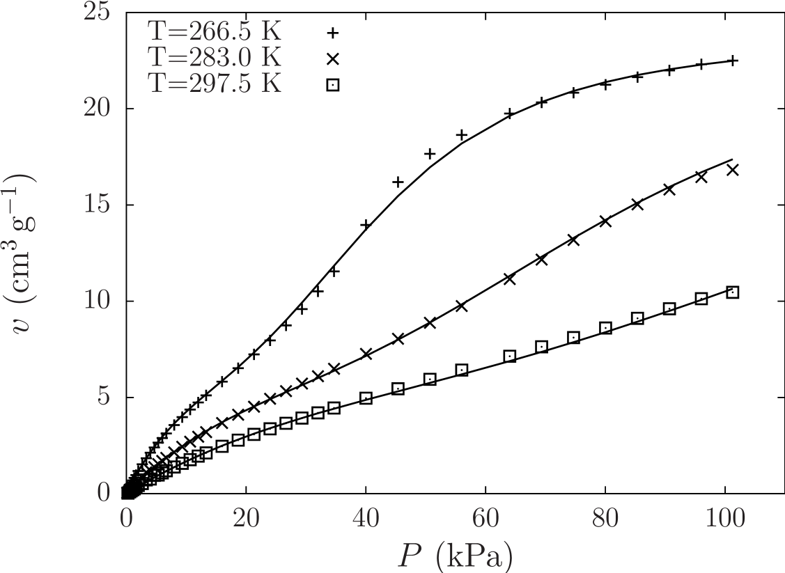
Figure 1:

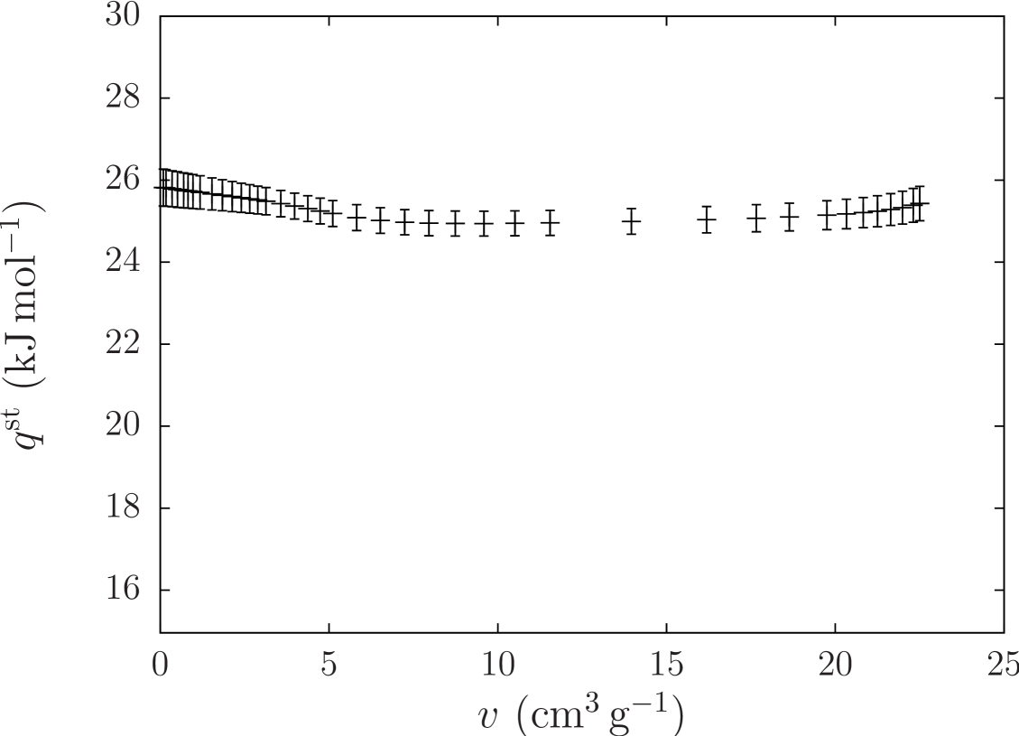
Figure 2:

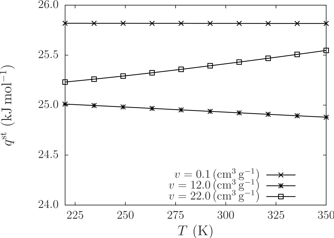
Figure 3:

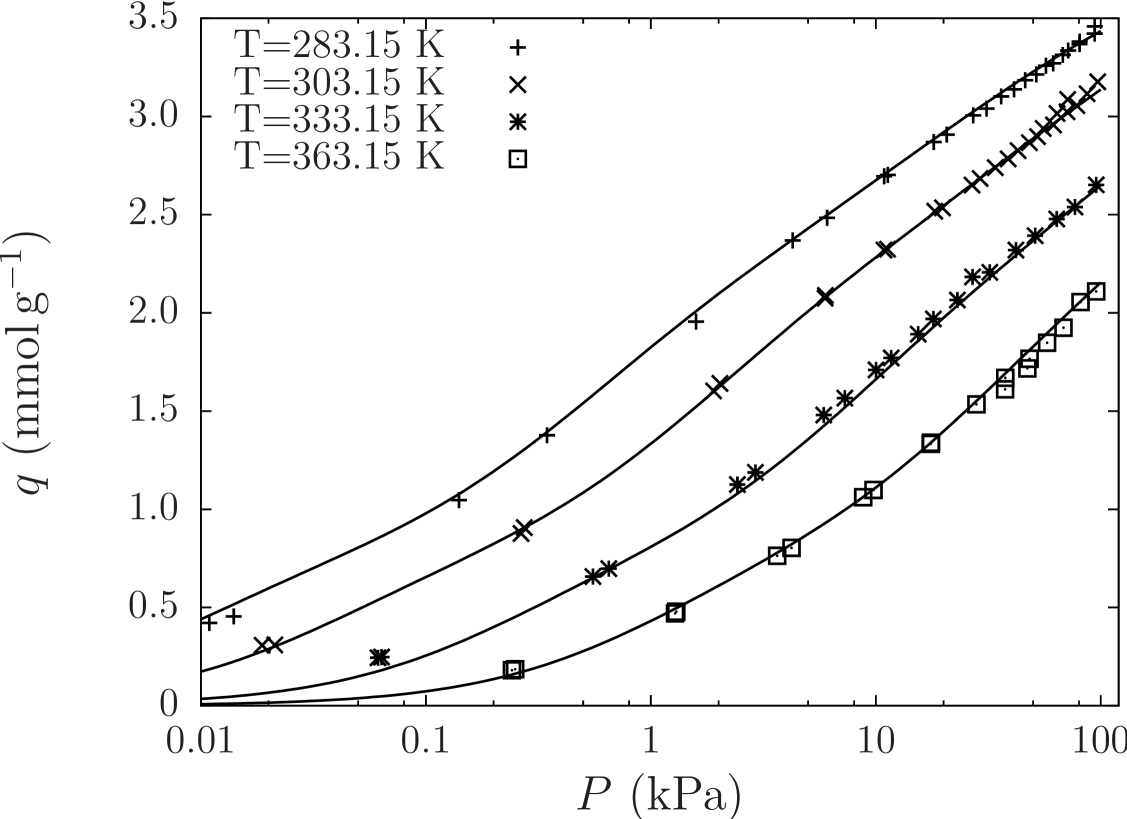
Figure 4:

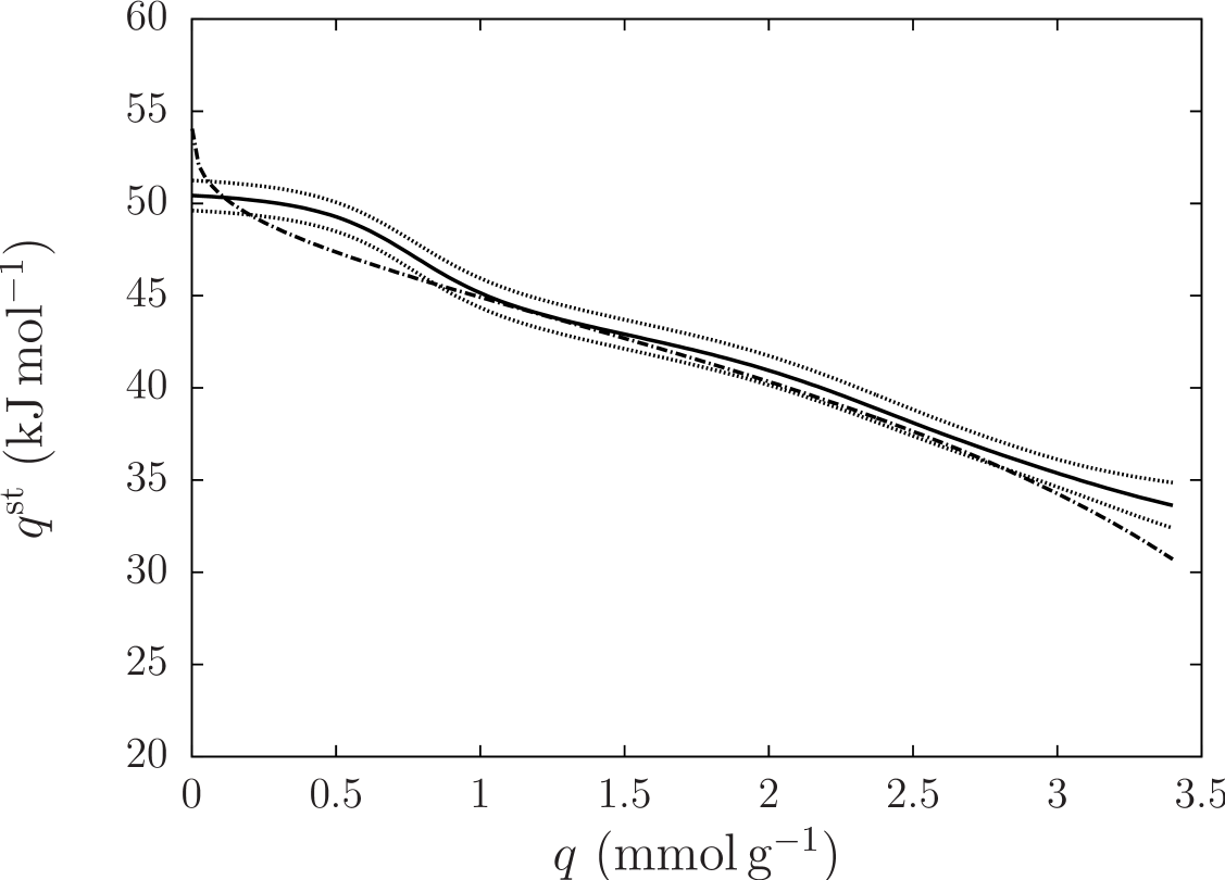
Figure 5:

a)

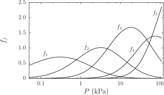
b)

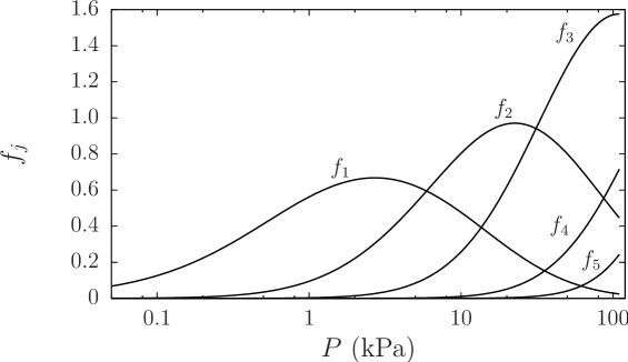
c)

Figure 6:

Table 1: Estimated parameters for several systems using Eq. 18.^a,b,c,d

	$q_{\mathrm{m}}$ (or $v$)	$\ln K^{\circ}$	$-10^{-3}\times\Delta h_{j}/R\,$	$D$	Temperature	Pressure
System	$\mathrm{mmol\,g^{-1}}$ (or $\mathrm{cm^{3}\,g^{-1}}$)		$\mathrm{K}$	$\%$	range (K)	range (kPa)
$\mathrm{SF_{6}}$+W-A(673)[4]	$23.89\pm 0.44$	$-13.67\pm 0.16$	$3.107\pm 0.055$	2.97	266.5-297.5	0.1-100
$l=1$			$6.112\pm 0.077$
			$8.08\pm 0.50$
			$11.62\pm 0.32$
$\mathrm{C_{3}H_{8}}$+W-A[4]	$34.6\pm 3.9$	$-14.65\pm 0.30$	$3.391\pm 0.096$	3.2	267-298	0.1-100
$l=1$			$7.472\pm 0.097$
			$10.8\pm 0.23$
			$14.8\pm 0.60$
			$17.9\pm 0.48$
$\mathrm{HFC}$-227ea+AC[42]	$3.87\pm 0.27$	$-16.67\pm 0.27$	$6.066\pm 0.098$	2.36	283.15-363.15	0.01-100
$l=0$			$11.39\pm 0.19$
			$16.38\pm 0.32$
			$20.82\pm 0.45$
			$24.71\pm 0.68$
$\mathrm{HFP}$+AC[42]	$3.87\pm 0.20$	$-15.66\pm 0.20$	$5.429\pm 0.075$	2.53	283.15-363.15	0.01-100
$l=0$			$10.15\pm 0.15$
			$14.68\pm 0.23$
			$18.69\pm 0.32$
			$22.33\pm 0.45$
$\mathrm{CO_{2}}$+ZC[19]	$4.82\pm 0.39$	$-15.71\pm 0.29$	$5.03\pm 0.10$	3.84	273.15-353.15	0.05-100
$l=1$			$9.39\pm 0.20$
			$13.45\pm 0.31$
			$17.00\pm 0.43$
$\mathrm{CO_{2}}$+SG[6]	$14.5\pm 1.0$	$-15.22\pm 0.10$	$3.068\pm 0.030$	1.47	278-328	50-3400
$l=4$			$5.759\pm 0.052$
			$8.454\pm 0.094$
			$10.87\pm 0.12$

^a In all cases, $P^{0}$ is expressed in kPa.
^b Abbreviations: activated carbon (AC), 1,1,1,2,3,3,3-heptafluoropropane (HFC-227a), hexafluoropropene (HFP), zeocarbon (ZC), silica gel (SG).
^c The parameters $\Delta h_{j}$ are tabulated in increasing order of $j$, e.g., for the $\mathrm{SF_{6}}$+W-A(673) system, $\Delta h_{1}/R=-3.107\times 10^{3},\,\Delta h_{2}/R=-6.112\times 10^{3}$, and so on.
^d For $\mathrm{SF_{6}}$+W-A(673) and $\mathrm{C_{3}H_{8}}$+W-A systems, the saturation is expressed in $\mathrm{cm^{3}\,g^{-1}}$ at 101.325 kPa and 273.15 K, and for the remaining systems it is expressed in $\mathrm{mmol\,g^{-1}}$.

Table 2: Estimated parameters for the adsorption data presented by Watson et al.[41] using Eq. 16 (l=0).^a,b,c

	$q_{\mathrm{m}}$	$\ln R_{j}^{\circ}$	$-10^{-3}\times\Delta\overline{h}_{j}/R\,$	$D$	Temperature	Pressure
System	$\mathrm{mmol\cdot g^{-1}}$		$\mathrm{K}$	$\%$	range (K)	range (kPa)
$\mathrm{CH_{4}}$+MSC	$4.412\pm 0.067$	$-14.4\pm 1.5$	$2.81\pm 0.41$	2.29	148-298	1-4000
		$-13.88\pm 0.48$	$1.92\pm 0.13$
$\mathrm{CO_{2}}$+MSC	$5.87\pm 0.14$	$-13.7\pm 1.3$	$3.26\pm 0.40$	1.41	223-323	25-5200
		$-14.00\pm 0.83$	$2.94\pm 0.25$
		$-16.07\pm 0.82$	$3.29\pm 0.22$
		$-19.46\pm 0.58$	$3.58\pm 0.17$
$\mathrm{N_{2}}$+MSC	$5.75\pm 0.12$	$-15.6\pm 1.1$	$2.71\pm 0.31$	3.14	115-298	0.01-5000
		$-14.03\pm 0.45$	$1.725\pm 0.099$
		$-18.3\pm 1.0$	$1.79\pm 0.15$

^a In all cases, $P^{0}$ is expressed in kPa.
^b Abbreviation: molecular sieving carbon (MSC).
^c As in 1, the parameters $\ln R_{j}^{\circ}$ and $\Delta\overline{h}_{j}$ are tabulated in increasing order of $j$, for example, for the $\mathrm{CH_{4}}$+MSC system, $\ln R_{1}^{\circ}=-14.4,\,\ln R_{2}=-13.88$, $\Delta\overline{h}_{1}/R=-2.81\times 10^{3},\,\Delta\overline{h}_{2}/R=-1.92\times 10^{3}$.

References

- Aranovich et al. [2004] G. L. Aranovich, J. S. Erickson, and M. D. Donohue. J. Chem. Phys., 120:5208–5216, 2004.
- Ayappa [1999] K. G. Ayappa. J. Chem. Phys., 111:4736–4742, 1999.
- Ayappa et al. [1999] K. G. Ayappa, C. R. Kamala, and T. A. Abinandanan. J. Chem. Phys., 110:8714–8721, 1999.
- Bandosz et al. [1996] T. J. Bandosz, J. Jagiełło, and J. A. Schwarz. J. Chem. Eng. Data, 41:880–884, 1996.
- Bates and Watts [1988] D. M. Bates and D. G. Watts. Nonlinear Regression Analysis and its Applications. Wiley, New York, 1988.
- Berlier and Frère [1997] K. Berlier and M. Frère. J. Chem. Eng. Data, 42:533–537, 1997.
- Boddenberg et al. [1997] B. Boddenberg, G. U. Rakhmatkariev, and R. Greth. J. Phys. Chem. B, 101:1634–1640, 1997.
- Boddenberg et al. [2002] B. Boddenberg, G. U. Rakhmatkariev, S. Hufnagel, and Z. Salimov. Phys. Chem. Chem. Phys., 4:4172–4180, 2002.
- Czepirsky and Jagiełło [1989] L. Czepirsky and J. Jagiełło. Chem. Eng. Sci., 44:797–801, 1989.
- Duong [1998] D. D. Duong. Adsorption Analysis: Equilibria and Kinetics. Imperial College Press, London, 1998.
- Gregg and Sing [1982] S. J. Gregg and K. S. W. Sing. Adsorption, Surface Area and Porosity. Academic Press, London, 1982.
- Hill [1953] T. L. Hill. J. Phys. Chem., 57:324–329, 1953.
- Hill [1956] T. L. Hill. Statistical Mechanics. McGraw–Hill, New York, 1956.
- Hill [1960] T. L. Hill. An Introduction to Statistical Thermodynamics. Addison–Wesley, Reading, MA, 1960.
- Jagiełło et al. [1995] J. Jagiełło, T. J. Bandosz, K. Putyera, and J. A. Schwarz. J. Chem. Eng. Data, 40:1288–1292, 1995.
- Kamat and Keffer [2002] M. R. Kamat and D. Keffer. Mol. Phys., 100:2689–2701, 2002.
- Kinnlburgh [1986] D. G. Kinnlburgh. Environ. Sci. Technol., 20:895–904, 1986.
- Langmuir [1918] I. Langmuir. J. Am. Chem. Soc., 40:1361–1403, 1918.
- Lee et al. [2002] J. Lee, J. Kim, J. Kim J. Suh, J. Lee, and C. Lee. J. Chem. Eng. Data, 47:1237–1242, 2002.
- Llano-Restrepo [2009] M. Llano-Restrepo. Adsorpt. Sci. Technol., 28:579–599, 2009.
- Llano-Restrepo [2010] M. Llano-Restrepo. Fluid Phase Equilibr., 293:225–236, 2010.
- Llano-Restrepo and Mosquera [2009] M. Llano-Restrepo and M. A. Mosquera. Fluid Phase Equilibr., 283:73–88, 2009.
- Narkiewicz-Michałek et al. [1999] J. Narkiewicz-Michałek, P. Szabelski, W. Rudziński, and A. S. T. Chiang. Langmuir, 15:6091–6102, 1999.
- Nikitas [1996] P. Nikitas. J. Phys. Chem., 100:15247–15254, 1996.
- Nitta et al. [1984] T. Nitta, M. Kuro-oka, and T. Katayama. J. Chem. Eng. Japan, 17:39–45, 1984.
- Prigogine and Defay [1954] I. Prigogine and R. Defay. Chemical Thermodynamics. Longmans Green and Co, New York, 1954.
- Ramirez-Pastor et al. [1999a] A. J. Ramirez-Pastor, T. P. Eggarter, V. Pereyra, and J. L. Riccardo. Phys. Rev. B, 59:11027–11036, 1999a.
- Ramirez-Pastor et al. [1999b] A. J. Ramirez-Pastor, V. D. Pereyra, and J. L. Ricardo. Langmuir, 15:5707–5712, 1999b.
- Riccardo et al. [2005] J. L. Riccardo, F. Romá, and A. J. Ramirez-Pastor. Appl. Surf. Sci., 252:505–511, 2005.
- Romá et al. [2005] F. Romá, J. L. Ricardo, and A. J. Ramirez-Pastor. Langmuir, 21:2454–2459, 2005.
- Ruthven [1971] D. M. Ruthven. Nat. Phys. Sci., 232:70–71, 1971.
- Ruthven and Loughlin [1972] D. M. Ruthven and K. F. Loughlin. J. Chem. Soc. Farad. Trans. I, 68:696–708, 1972.
- Ruthven and Wong [1985] D. M. Ruthven and F. Wong. Ind. Eng. Chem. Fund., 24:27–32, 1985.
- Seber and Wild [1989] G. A. F. Seber and C. J. Wild. Nonlinear Regression. Wiley, New York, 1989.
- Sips [1948] R. Sips. J. Chem. Phys., 16:490–495, 1948.
- Sips [1950] R. Sips. J. Chem. Phys., 18:1024–1026, 1950.
- Smith et al. [2005] J. M. Smith, H. C. Van Ness, and M. M. Abbott. Introduction to Chemical Engineering Thermodynamics. McGraw-Hill, New York, 2005.
- Stach et al. [1986] H. Stach, U. Lohse, H. Thamm, and W. Schirmer. Zeolites, 6:74–90, 1986.
- Steele [1963] W. A. Steele. J. Phys. Chem., 67:2016–2023, 1963.
- Toth [1971] J. Toth. Acta Chim. Acad. Sci. Hung., 69:311–328, 1971.
- Watson et al. [2009] G. Watson, E. F. May, B. F. Graham, M. A. Trebble, R. D. Trengove, and K. I. Chan. J. Chem. Eng. Data, 54:2701–2707, 2009.
- Yun et al. [2000] J. Yun, D. Choi, and Y. Lee. J. Chem. Eng. Data, 45:136–139, 2000.