Fractal dimension of a liquid flows predicted coupling an Eulerian-Lagrangian approach with a Level-Set method

Abstract

The fractal dimension of a liquid column is a crucial parameter in several models describing the main features of the primary break-up occurring at the interface of a liquid phase surrounded by the gas-flow. In this work, the deformation of the liquid phase has been numerically studied. The gas-phase is computed as a continuum in an Eulerian frame while the liquid phase is discretized in droplets Lagrangian tracked and coupled via the momentum equation with the surrounding gas flow. The interface is transported by the flow field generated because of the particle forcing and it is numerically computed using the Level-Set method. Finally, the fractal dimension of the interface is locally estimated and used as criterion for the model of the primary breakup.

I Introduction

The break-up of a liquid flow leads the evaporation process in a wide range of applications such as in combustion, exhaust gas post-treatment and other devices. The rate of break-up enhance the liquid evaporation since the surface/volume ratio increases. The atomization occurs according with two main mechanisms: the primary and the secondary break-up Wang08 .

Firstly, coherent structures detach from the liquid/gas interface up to break in spherical droplets because of either the Rayleigh-Taylor or Kelvin-Helmholtz instability. The instability is locally modulated by waves depending on the velocity and the pressure fluctuations induced on the smaller length scales because of the turbulence (primary break-up).

Thus, each droplet, occurring in the primary breakup, fragments up to evaporate because of the shear stress induced by the surrounding gas-flow (secondary breakup).

In the case of low pressure injection, the break-up depends mainly on the surface energy while the interface instability plays a negligible role. The surface energy could be estimated using a model based on the fractal dimension of the liquid/gas interface DeR09 . The connection between the shape of the liquid column and the atomization process has been pointed out in several experimental studies using the fractal dimension Grout07 ; Moyne08 ; Weixing00 . The topology of the core region is challenging to investigate using experiments since the measurements are affected by the resuspended droplets detaching from the liquid-gas interface.

Numerical simulation appears to be a promising tool for this purpose. In the last two decades there has been progress on this topic improving the numerical methods for the the solution of the governing equations of each phase and for the topological treatment of the fluid-gas interface. Following, the the most remarkable techniques used in literature have been depicted.

The Front Tracking Front1 , the Volume of Fluid method Vol1 and the Level-Set Level1 are the main front-capturing methods.

The Front Tracking method is based on the Lagrangian treatment of the interface that is described by ideal particle (markers). The markers are connected each other and they are moved like an ideal fluid particle. The connectivity between discrete elements covering the interface is not straightforward in three spatial dimensions. The drawback of this method depends on the collapsing, the stretching and the deformation of some discrete elements. These elements should be periodically replaced in order to preserve the curvature and the mass of the fluid confined by the interface. These difficulties vanish if the interface is described using methods in the Eulerian frame as the Volume of Fluid method or the Level-Set method.

In the Volume of Fluid method each phase is represented by the volume fraction of the fluid per each computational cell and the interface evolves according to the advection equation. Despite of the simplicity in describing the connectivity, a thickness of the interface is artificially introduced. Thus, the curvature and the surface tension are not well estimated. The advantage of this method consists in the accurate mass conservation. With the Level-Set method the interface is described by the iso-contour of an implicit function $\phi(\textbf{x})=0$, defined in all the points x of a fixed computational domain $\Omega$, whose evolution is governed by the advection equation. The interface, the outer region and the inner region are defined by $\phi(\textbf{x})=0$, $\phi(\textbf{x})>0$, $\phi(\textbf{x})<0$, respectively. The implicit function ensure the description of complex gas-fluid interface without the stringent conditions coming from the parametric representation of the surface. With the Level-Set method the interface is well defined and the surface tension is precisely predicted since depends on the gradient of the implicit function, only.

Traditionally, the Level-Set involves the numerical solution in the Eulerian frame for both the liquid and gas phases. This method fails for high Reynolds number because the steep gradients of density and viscosity across the interface requires a fine computational grid making tricky the fast simulation of such flows. Moreover, this procedure is prohibitive in the industrial applications, such as engine combustion, because the liquid column evolve in a wide region far away from the injector.

The Eulerian-Lagrangian approach is a strategy to make faster the simulations preserving a reasonable accuracy for the interface tracking. The gas-phase is computed as a continuum in an Eulerian frame while the liquid phase is discretized in droplets Lagrangian tracked and coupled via the momentum equation with the surrounding gas flow. The liquid particle has to be smaller enough to feel all the velocity fluctuations of the gas-phase in order to preserve as much as possible the instability effects induced on the liquid phase.

Once the velocity field has been computed both for the gas and liquid phases the interface is transported according to the Level-Set method. The advection velocity of the interface is equal to the velocity of the liquid particles along the interface. Finally, the fractal dimension of the liquid/gas interface is locally estimated using the box-counting procedure.

II Level-Set method

In three space dimension a closed surface separate the whole domain $\Omega$ into the inside domain $\Omega^{-}$ and the outside domain $\Omega^{+}$. The border between the inside domain and the outside domain is called the interface $\partial\Omega$. An implicit interface representation defines the interface as the iso-contour of some function $\phi(\textbf{x})$ with $\textbf{x}\in\Omega$. The interface, the outer region and the inner region are defined by $\phi(\textbf{x})=0$, $\phi(\textbf{x})>0$, $\phi(\textbf{x})<0$, respectively OsSe .

The gradient of the implicit function $\nabla\phi$ is perpendicular to the iso-contours of $\phi$. Therefore, $\nabla\phi$ evaluated at the interface is a vector that points in the same direction as the local unit (outward) normal n to the interface. Thus, the unit (outward) normal is:

$$\textbf{n}=\frac{\nabla\phi}{|\nabla\phi|}$$ (1)

for points on the interface.

The mean curvature of the interface $k$ is defined as the divergence of the normal $k=(\nabla\cdot\textbf{n})/2$ so that $k>0$ for convex regions, $k<0$ for concave regions, and $k=0$ for a plane. Using the definition of normal vector we obtain:

$$k=\frac{1}{2}\nabla\cdot\left(\frac{\nabla\phi}{|\nabla\phi|}\right)$$ (2)

Smoothness of the $\phi$ is a desiderable property especially in using numerical approximations. Signed distance functions are a subset of the implicit functions $\phi$ with the extra condition of $\nabla\phi(\textbf{x})=1$ enforced:

$$\phi(\textbf{x})=min(\textbf{x}-\textbf{x}_{i})\mbox{ $\textbf{x}\in\Omega$, $\textbf{x}_{i}\in\partial\Omega$}$$ (3)

Under these assumption the normal to the interface is:

$$\textbf{n}=\nabla\phi$$ (4)

and the mean curvature is:

$$k=(\nabla^{2}\phi)/2.$$ (5)

The signed distance function turns out to be a good choice, since steep and flat gradients as well as rapidly changing features are avoided as much as possible. The evolution of the interface is governed by the following equation:

$$\phi_{t}+\textbf{v}\cdot\nabla\phi=0,$$ (6)

where v is the velocity of the liquid phase computed at the interface. Once the interface location is known the Navier-Stokes equation are solved in the gas-phase and the liquid-phase is Lagrangian tracked.

III Numerical method for the gas-phase

The integral form of the conservative equations applied to the control volume $V_{0}$ with a boundary surface $S_{0}$ and the unity normal vector pointing outward to the surface $S_{0}$ defined by n is:

$$\int_{V_{0}}\frac{\partial\rho}{\partial t}dV+\int_{S_{0}}\rho\textbf{u}\cdot\textbf{n}dS=0$$ (7)

and the momentum equation is:

$$\int_{V_{0}}\frac{\partial\rho\textbf{u}}{\partial t}dV + \int_{S_{0}}\rho\textbf{u}\textbf{u}\cdot\textbf{n}dS=$$ (8)

$$= -\int_{S_{0}}p\textbf{n}dS+\int_{S_{0}}\mu\nabla^{2}\textbf{u}\cdot\textbf{n}dS$$

$$+\int_{V_{0}}\rho\textbf{g}dV+\int_{V_{0}}\textbf{f}_{liquid}dV$$

where $\rho$, $\mu$ are the density and the dynamic viscosity, respectively. The flow velocity is u, the gravity vector is g , the flow pressure is $p$, the time is $t$ and the feedback forcing induced by the liquid phase is $\textbf{f}_{liquid}$.

The numerical solver (KIVA) of the gas-phase equations is based on a finite volume method. Spatial difference approximations are constructed by the control-volume or integral-balance approach, which largely preserves the local conservation properties of the differential equations. In the finite-volume approximations of KIVA, velocities are located at the vertices and the scalar quantities are located at cell centers. Surface and volume integrals are approximated using suitable quadrature formulae. Volume integrals of gradient or divergence terms are converted into surface area integrals using the divergence theorem. The volume integral of a time derivative maybe related to the derivative of the integral by means of Reynolds’ transport theorem. Volume and surface area integrals are performed under the assumption that the integrands are uniform within cells or on cell faces. Thus area integrals over surfaces of cells become sums over cell faces $i$:

$$\int_{\textbf{S}}\textbf{F}d\textbf{A}=\sum_{i}\textbf{F}d\textbf{A}$$ (9)

The effect of turbulence is take into account with a standard version of $k-\epsilon$ turbulence model modified to include liquid-turbulence interaction. Evaporating liquid phase is represented by a discrete-particle technique The momentum exchange is treated by implicit coupling procedures to avoid the prohibitively small time steps that would otherwise be necessary. Turbulence effects on the droplets are accounted. When the time step is smaller than the droplet turbulence correlation time, a fluctuating component is added to the local mean gas velocity when calculating each particle’s momentum exchange with the gas. When the time step exceeds the turbulence correlation time, turbulent changes in droplet position and velocity are chosen randomly from analytically derived probability distributions for these changes. The temporal differencing is performed with a first-order scheme.

IV Numerical method for the liquid-phase

XXX-stochastic method

The liquid phase has been modelled like a cloud of rigid spherical particles with all the forces applied on the particle centroid. The time history of each particle is numerically computed (Lagrangian particle tracking) using a model for the momentum equation with drag and gravity force, only Maxey ; Camp :

$$m_{p}\frac{dv}{dt}=\frac{1}{2}C_{D}\frac{\pi d_{p}^{2}}{4}\rho|\textbf{u}-\textbf{v}|(\textbf{u}-\textbf{v})+m_{p}\textbf{g}$$ (10)

in which $m_{p}$ is the mass, $d_{p}$ is the diameter and $C_{D}$ is the drag coefficient.

The slight deviation from the Stokes flow has been taken into account with the drag correction $C_{D}$ proposed by Shiller and Naumann Shi33 for particle with Reynolds number $Re_{p}<1000$.

$$C_{D}=\frac{24}{Re_{p}}\left(1+\frac{1}{6}Re_{p}^{2/3}\right)\hskip 2.84544pt;\hskip 14.22636ptRe_{p}=\frac{\rho d_{p}|\textbf{u}-\textbf{v}|}{\mu}$$ (11)

We can rearrange the equation (Eq. 10) as follows:

$$\frac{dv}{dt}=\frac{1}{\tau_{p}}\left(1+\frac{1}{6}Re_{p}^{2/3}\right)(\textbf{u}-\textbf{v})+\textbf{g},\hskip 14.22636pt\tau_{p}=\frac{\rho_{p}d_{p}^{2}}{18\mu}$$ (12)

The particle is selectively sensitive to the flow velocity fluctuations induced by the turbulence. This response of a particle to the surrounding gas velocity field is estimated by the Stokes number $St=\tau/\tau_{p}$, in which $\tau$ is the time scale of the eddy interacting with the particle characterized by the relaxation time $\tau_{p}$. The time scale $\tau=L/U$ depends on the characteristics length $L$ and velocity $U$ of the gas-phase.

Specifically, the droplet with very small Stokes number will simply be a flow tracers $St<<1$ (lighter particle). For increasing the Stokes number, the particle trajectory will diverge from the flow stream-line until the particle motion will be completely independent from the surrounding flow $St>>1$ (heavier particle). If the Stokes number is order one the particle has the maximum interaction with the velocity fluctuation of the gas-phase Sq90 . In Figure 1 it is qualitatively depicted the particle-eddy interaction in which the particle velocity approaches quickly to the fluid velocity for decreasing the Stokes number.

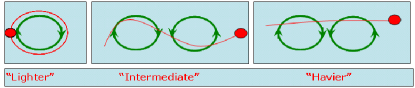
Figure 1: Qualitatively description of the interaction between particle and vortices. $St<<1$ - lighter, $St\sim O(1)$ - intermediate, $St>>1$ - heavier.

Particle behavior depending on the Stokes number can analytically depicted in the limit of one-dimensional Stokes flow ($Re_{p}<<1$), neglecting the gravity for a particle dispersed in a gas-phase with constant velocity $u=u_{0}$. Under this hypothesis the equation 12 in dimensionless form read:

$$\frac{dv^{*}}{dt^{*}}=\frac{1}{St}\left(u^{*}_{0}-v^{*}\right)$$ (13)

where $u^{*}_{0}=u_{0}/U$, $v^{*}=v/U$ and $t^{*}=tU/L$. The solution of the previous equation (Eq. 14), in the case of initial particle velocity equal to zero, has been plotted in Fig. 2.

$$v^{*}=u^{*}_{0}\left(1-e^{-t^{*}/St}\right)$$ (14)

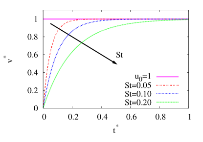
Figure 2: Parametric solution of Eq. 14 for $u^{*}_{0}=1$ and three Stokes numbers: $St=0.05$, $St=0.1$, $St=0.2$

In this scenario, the particle diameter, in the Lagrangian model of the liquid phase, should be small enough in order to make each particle sensitive to the velocity fluctuation of the smallest vortical scale. In the turbulent regime the smallest vortical scale is defined by the dissipative length scale $\eta$, the velocity $U_{k}$ and the time $\tau_{k}$. Following the Kolmogorov theory the large scale ($U$, $L$, $\tau$) and the dissipative scale ($U_{k}$, $L_{k}$, $\tau_{k}$) are connected according to the following relations:

$$\eta=\left(\frac{\nu^{3}}{\epsilon}\right)^{1/4},\hskip 14.22636ptU_{k}=(\nu\epsilon)^{1/4}\hskip 14.22636pt\tau_{k}=\left(\frac{\nu}{\epsilon}\right)^{1/2};$$ (15)

in which $\epsilon=U^{3}/L$ assess the energy in the whole domain. Thus, the equation 15 read:

$$\frac{\eta}{L}=Re^{-3/4},\hskip 14.22636pt\frac{U_{k}}{U}=Re^{-1/4}\hskip 14.22636pt\frac{\tau_{k}}{\tau}=Re^{-1/2};$$ (16)

where $Re=(UL)/\nu$ is the Reynolds number evaluated at the large scale.

The Stokes number based on the Kolmogorov scales $St_{k}$ is:

$$St_{k}=\frac{\tau_{p}}{\tau_{k}}=\frac{\tau_{p}}{\tau}\frac{\tau}{\tau_{k}}=StRe^{1/2}$$ (17)

Thus, if $St_{k}<<1$ each particle of the liquid phase takes into account the instability effects occurring at the liquid/gas interface since the liquid particle is sensitive to the velocity fluctuation in the whole range of the turbulent scales occurring in the computational domain. For this reason, the particle diameter should be satisfy the equation 18:

$$St_{k}<<1\Rightarrow StRe^{1/2}<<1\Rightarrow$$

$$\Rightarrow d_{p}<<3\sqrt{2}\cdot L\cdot\sqrt{\frac{\rho}{\rho_{p}}}\cdot Re^{-3/4}$$ (18)

V Results

The time and the spatial evolution of the gas/liquid interface has been estimated using the Level-Set method. According to the Level-Set method, the evolution of the interface is governed by the advection equation 6. The initial condition of Eq. 6 is $R_{s}=d_{i}/2$, in which $R_{s}$ is the radius of curvature of the liquid phase and $d_{i}/2$ is the radius of the injector. The liquid particles are injected into the gas phase within a prescribed maximum angle $\alpha_{i}$. In order to enforce both the angle $\alpha_{i}$ and the injector diameter $d_{i}$ the particles have been dispersed at the following distance from the orifice:

$$h_{i}=\frac{d_{i}}{2}tg\left(\frac{\alpha}{2}\right)$$ (19)

The center of the sphere, with radius $R_{s}$, is defined in a Cartesian frame by $(x_{s},y_{s},z_{s})$, where $y_{s}=y_{i}$ and $x_{s}=x_{i}$, while $z_{s}$ depends on $R_{s}$ and $\alpha_{i}$ as follows:

$$z_{s}=z_{i}-\sqrt{R_{s}^{2}-\frac{d_{i}^{2}}{4}}+h_{i}$$ (20)

$$z_{s}=z_{i}-\sqrt{R_{s}^{2}-\frac{d_{i}^{2}}{4}}+\frac{d_{i}}{2}tg\left(\frac{\alpha_{i}}{2}\right)$$ (21)

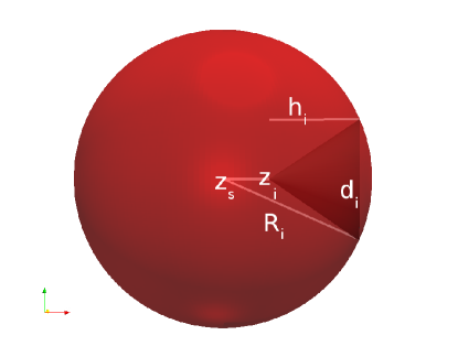
Figure 3: Initial level-set iso-contour.

The numerical simulations have been carried out using an injector with diameter $d_{i}=1.58\cdot 10^{-4}$ $[m]$ crossed by a liquid with velocity $U=27$ $[m/s]$ and density $\rho_{p}=10^{3}$ $[Kg/m^{3}]$. For such flow the Reynolds number is equal to $Re=U\cdot d_{i}/\mu=4.310^{3}$. According to equation 18 the particle diameter should be $d_{p}<<6.9\cdot 10^{-9}$ $[m]$, thus the liquid jet has been discretized using droplets with diameter $d_{p}=10^{-9}$ $[m]$.

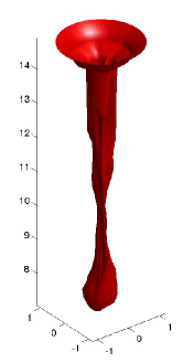
Figure 4: Interface of the liquid jet.

The liquid jet is organized in an elongated structure with inhomogeneous shape modulated by the velocity fluctuations leading the instability at the liquid/gas interface. The degree of complexity of the interface has been measured using the fractal dimension. The fractal dimension is the control parameter in several breakup models since it is the integral measure of the distortion of the liquid jet DeR09 . The fractal dimension can be regarded as the general case of the Eulerian dimension. If we take an object residing in Euclidean dimension $D$ and reduce its linear size by $1/r$ in each spatial direction, its measure (length, area, or volume) would increase to $N=r^{D}$ times the original. This is pictured in the next figure.

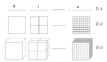
Figure 5: Examples of figures with integer dimension. Lecture notes of Fluid Dynamics by R. Verzicco http://ime115.poliba.it/verzicco/

We consider $N=r^{D}$, take the log of both sides, and get

$$log(N)=Dlog(r)$$ (22)

If we solve for D.

$$D=log(N)/log(r)$$ (23)

In the Eulerian frame $D$ is an integer number. Fractals, which are irregular geometric objects, have a fractional dimension. This theoretical criterion is not straightforward to compute the fractal dimension in numerical computation. For this reason, the computation of the fractal dimension of the liquid jet is based on the box-counting procedure. To calculate the fractal dimension using the box-counting algorithm the liquid/gas interface has been placed on a grid. Then, the number of blocks crossed by the surface has been stored and iteratively computed for resizing grids. The fractal dimension $D$ is the slop of the best fit in a log-log scale plane of the number of boxes $N(s)$ as function of the size $s$ of the resized grids. The box-counting method is widely used since it can measure geometry that are not self-similar.

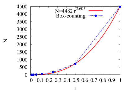
Figure 6: Best fit of the fractal dimension using the box counting method.

The slope of the best fit is equal to $D=2.605$ and it represent the degree of complexity of the liquid jet surface.

VI Summary and conclusions

References

- (1) Wang,Y., Im, k., Fezzaa,k., 2008. Similarity between the Primary and Secondary Air-Assisted Liquid Jet Breakup Mechanisms. Phys. Rev. Lett. 100, 154502.
- (2) De Risi, A., Donateo, T., Sciolti, A., Caló, M., Gaballo, M. R., 2009. A new energy-based model for the prediction of primary atomization of urea-water sprays. SAE International, 2009-01-0902
- (3) Grout, S., Dumouchel, C., Cousin, J., Nuglisch, H. 2007. Fractal analysis of atomizing liquid flows. Int. J. Multiphase Flow. 33, 1023-1044.
- (4) Le Moyne, L., Freire, V., Queiros Conde, D., 2008. Fractal dimension and scale entropy applications in a spray. Chaos Solitons & Fractals. 38, 696-704.
- (5) Weixing, Z., Tiejun, Z., Tao, W., Zunhong, Y., 2000. Application of fractal geometry to atomization process. Chehemical Engineering J., 78, 193-197.
- (6) Unverdi, S.O., Tryggvason, G., 1992. A front-tracking method for viscous, incompressible multi-fluid flows. J. Comput. Phys. 100, 25–37.
- (7) Gueyffier, D., Li, J., Nadim, A., Scardovelli, S., Zaleski, S., 1999. Volume of Fluid interface tracking with smoothed surface stress methods for three-dimensional flows. J. Comput. Phys. 152, 423–456.
- (8) Osher, S., Sethian, J.A., 1988. Fronts propagating with curvature-dependent speed: algorithms based on Hamilton–Jacobi formulations. J. Comput. Phys. 79, 12–49.
- (9) Osher, S., Sethian, J., 1988. Fronts propagation with curvature dependent speed: algorithms based on Hamilton-Jacobi formulations. J. Comput. Phys. 79, 12–49.
- (10) Maxey, M. R., Riley, J. J., 1983. Equation of motion for a small rigid sphere in a nonuniform flow. Phys. Fluids, 26(4)883-889.
- (11) Campolo, M., Salvetti, M. V., Soldati, A., 2004. Mechanisms for microparticle dispersion in a jet in crossflow. AIChE Journal, 51(1)28-43.
- (12) Shiller, L., Naumann, A., 1933. Über die grundlegenden berechungen bei der schwerkreftaufbereitung. Ver Deut. Ing., (77)318.
- (13) Squires, K. D., Eaton, J. K., 1990. Particle response and turbulence modification in isotropic turbulence. Phys. Fluids A, (2)1192-1203.
- (14) Elghobaschi, S., Truesdell, G. C., 1993. On the two-way interaction between homogeneous turbulence and dispersed solid particles. Phys. Fluids A, (5)1790-1810.
- (15) Boivin, M., Simonin, O., Squires, K., 1998. Direct numerical simulation of turbulence modulation by particles in isotropic turbulence. J. Fluid Mech., (375)235-263.
- (16) Elghobaschi, S., Truesdell, G. C., 1992. Direct simulation of particle dispersion in a decaying isotropic turbulence. J. Fluid Mech., (242)655-700.