Evaluation of Israel-Stewart parameters in lattice gauge theory

Abstract:

Navier-Stokes equations are known as hydrodynamic equations which take account of effects of dissipations. There are, however, problems in the relativistic Navier-Stokes equations, i.e. the equations violate causality. Israel-Stewart equations, which evade the problems of Navier-Stokes equations by introducing new parameters, such as the relaxation times, have recently been used in describing the space-time evolution of the quark-gluon plasma produced in high energy heavy ion collisions. The viscosities and the relaxation times are related to each other by imposing entropy constraints on the system. According to Boltzmann-Einstein principle, the probability distribution of the fluctuation in the energy-momentum tensor is related to the entropy of the system. Applying this principle to the entropy in Israel-Stewart theory, one can obtain the ratios of the viscosities to the relaxation times. We evaluate the ratios of the viscosities to the relaxation times in SU(3) lattice gauge theory.

1 Introduction

The new form of matter created at RHIC (Relativistic Heavy Ion Collider) has provided physicists unexpected findings. One of the most impressive results is that the new matter, which is referred to as quark-gluon plasma (QGP), behaves like perfect fluid near critical temperature $T_{\mathrm{c}}$. The space-time evolution of QGP in high energy heavy ion collisions seems to be understood quantitatively by relativistic ideal hydrodynamics. However, relativistic dissipative hydrodynamics is needed for more quantitative description of the real QGP evolution since QGP has small but nonzero viscosities.

The simplest relativistic dissipative hydrodynamics is the first order theory which is a relativistic extension of Navier-Stokes theory [1, 2]. This theory, however, accompanies problems associated with causality violation [3]. Instead of the first order theory, second order dissipative hydrodynamics, especially Israel-Stewart (IS) theory [4], has been recently actively studied. IS theory avoids the problems by introducing second order terms of dissipation, which physically represent relaxation effects to the solution of the first order theory. As an inevitable consequence of introducing the second order terms, however, IS theory includes many phenomenological parameters in addition to the three transport coefficients in the first order theory. These parameters cannot be determined within hydrodynamics. Other approaches based on microscopic theories are needed to determine the parameters.

“Perfect fluid”-like behavior of QGP indicates that quarks and gluons strongly interact with each other in QGP near $T_{\mathrm{c}}$ [5]. The properties of QGP near $T_{\rm c}$ are not within the reach of perturbation theory, since perturbative expansion is poorly converging at large couplings. At present, lattice gauge theory is the only systematic approach which can calculate physical quantities in such a non-perturbative region. There have been done several attempts to measure transport coefficients with numerical simulations on the lattice [6, 7, 8]. These analyses evaluate transport coefficients using Kubo formulae, which relate transport coefficients to the correlation functions of the energy-momentum tensors in Minkowsiki space-time. On the other hand, on the lattice one can calculate correlation functions in Euclidean space-time. An analytic continuation from imaginary-time correlation functions to real-time ones therefore is required in this strategy. In previous studies [6, 7, 8], nontrivial ansätze have been adopted for the form of real-time spectral function in order to perform this analytic continuation. Validity of such ansätze, however, should be carefully examined.

In the present study, we attempt to constrain phenomenological parameters in IS theory on the lattice using a method proposed in Refs. [9, 10]. In this method, ratios between the viscosities and the relaxation times in IS equations are related to static fluctuations of stress tensor in equilibrium through Boltzmann-Einstein principle. Since one does not use temporal correlation functions in this method, one can avoid the difficulty in the analytic continuation. The main objective of this work is to evaluate these ratios in SU(3) gauge theory on the lattice and to reduce the number of phenomenological parameters in IS theory.

2 Israel-Stewart theory

In this section, we overview relativistic dissipative hydrodynamics, especially Israel-Stewart (IS) theory [4, 11]. Basic equations of hydrodynamics are local conservation laws of the energy-momentum and the net charge,

$$\partial_{\mu}T^{\mu\nu}=0,$$ (1)

$$\partial_{\mu}N^{\mu}=0.$$ (2)

Using arbitrary 4-velocity of fluid $u^{\mu}$ normalized as $u^{\mu}u_{\mu}=1$ and the projection onto 3-dimensional space $\Delta^{\mu\nu}=g^{\mu\nu}-u^{\mu}u^{\nu}$, the energy-momentum tensor $T^{\mu\nu}$ and the charge density $N^{\mu}$ are decomposed as

$$T^{\mu\nu} = \epsilon u^{\mu}u^{\nu}-(p+\Pi)\Delta^{\mu\nu}+W^{\mu}u^{\nu}+W^{\nu}u^{\mu}+\pi^{\mu\nu},$$ (3)

$$N^{\mu} = nu^{\mu}+V^{\mu},$$ (4)

where $\epsilon$, $p$, and $n$ are the energy density, pressure, and charge density, respectively. Eckart used the particle flow as 4-velocity $u^{\mu}$,

$$u^{\mu}\equiv\frac{N^{\mu}}{\sqrt{N_{\mu}N^{\mu}}},$$ (5)

which is called Eckart (particle) frame, and $V^{\mu}$ vanishes in this frame. Landau-Lifshitz employed the energy flow for $u^{\mu}$,

$$u^{\mu}\equiv\frac{T^{\mu}_{\nu}u^{\nu}}{\sqrt{u^{\alpha}T_{\alpha}^{\beta}T_{\beta\gamma}u^{\gamma}}}.$$ (6)

This is Landau-Lifshitz (energy) frame, and $W^{\mu\nu}$ vanishes in this frame. While the values of $W^{\mu}$ and $V^{\mu}$ depend on the choice of the frame,

$$q^{\mu}=W^{\mu}-\frac{\epsilon+p}{n}V^{\mu},$$ (7)

i.e. heat flow in the particle frame, is frame independent in first order.

The basic idea of Israel [12] for a phenomenological derivation of second order hydrodynamics is to incorporate the effects of dissipation into the entropy current $s^{\mu}$. Under the hydrodynamic assumption, i.e. that nonequilibrium states are characterized by hydrodynamic variables, $T^{\mu\nu}$ and $N^{\mu}$, the entropy current should be given by $s^{\mu}=s^{\mu}(T^{\rho\sigma},N^{\rho})$. Assuming further that one can expand $s^{\mu}$ for nonequilibrium states by the power series of $\Pi$, $\pi^{\mu\nu}$, and $q^{\mu}$, the most general form of entropy current at second order in dissipative terms, $\Pi$, $\pi^{\mu\nu}$, and $q^{\mu}$, reads,

$$s^{\mu}=\frac{s_{\mathrm{eq}}}{n}N^{\mu}+\frac{q^{\mu}}{T}+Q^{\mu},$$ (8)

where

$$Q^{\mu}=-\frac{u^{\mu}}{2T}\left(\beta_{0}\Pi^{2}-\beta_{1}q_{\nu}q^{\nu}+\beta_{2}\pi_{\nu\lambda}\pi^{\nu\lambda}\right)-\frac{\alpha_{0}\Pi q^{\mu}}{T}+\frac{\alpha_{1}\pi^{\mu\nu}q_{\nu}}{T},$$ (9)

represents the second order contribution to entropy, and $s_{\mathrm{eq}}$ and $T$ are the entropy density in equilibrium and the local temperature of the system, respectively. Here, $\beta_{i}$ and $\alpha_{i}$ are phenomenological coefficients and are not determined by the hydrodynamic assumption.

Requiring the second law of thermodynamics, $\partial_{\mu}s^{\mu}\geq 0$, one can constrain the macroscopic equations that hydrodynamic variables follow. If we neglect the second order term in $s^{\mu}$, the second law and linearity lead to the first order hydrodynamic equations including three transport coefficients, shear and bulk viscosities $\eta$ and $\zeta$, and heat conductivity $\lambda$. Similarly, when one recovers the second order terms, $Q^{\mu}$, in Eq. (8), the second law leads to constraints including second order terms. IS equations are defined so as to satisfy these constraints [4, 12].

IS equations include terms $D\Pi$ and $D\pi$ with $D\equiv u_{\mu}\partial^{\mu}$ being the derivative along $u^{\mu}$. These terms give rise to relaxation effects to the solution of first order equations, and cure the causality problem of the first order theory. Proportional coefficients of these terms are given by

$$\tau_{\Pi}=\beta_{0}\zeta,\qquad\tau_{\pi}=2\beta_{2}\eta,$$ (10)

respectively, which physically represent the time scale of the relaxation in each channel and are called relaxation times. Equation (10) means that the ratios between viscosities and the relaxation times are related to proportional coefficients in the entropy current, $\beta_{0}$ and $\beta_{2}$, as

$$\beta_{0}=\frac{\tau_{\Pi}}{\zeta},\qquad\beta_{2}=\frac{\tau_{\pi}}{2\eta}.$$ (11)

3 Boltzmann-Einstein principle

In what follows, we try to evaluate the ratios in Eq. (11) on the lattice by connecting $\beta_{0}$ and $\beta_{2}$ to fluctuations of stress tensor using Boltzmann-Einstein (BE) principle.

The entropy and the number of microscopic states in equilibrium are related to each other by Boltznmann relation

$$S(\vec{a})=\ln W(\vec{a}),$$ (12)

where $\vec{a}=\left\{a_{1},a_{2},a_{3},...\right\}$ represents the set of state variables of the system, and $S(\vec{a})$ and $W(\vec{a})$ are the entropy and the number of microscopic states, respectively, in the system specified by state variables $\vec{a}$. To put it another way, the number of microscopic states is given by BE principle [9, 10],

$$W(\vec{a})=\exp[S(\vec{a})].$$ (13)

Since the probability that one of the state variables $a_{i}$ takes a certain value, $A$, in equilibrium is given by

$$P(a_{i}=A)=\frac{W(a_{i}=A)}{\sum W(\vec{a})},$$ (14)

BE principle means that the probability distribution of state variables in equilibrium is governed by the entropy, provided that the entropy $S(\vec{a})$ is defined.

¿From Eqs. (8) and (9), the entropy in unit volume $s$ in IS theory at rest frame $u^{\mu}$ is given by

$$s=u_{\mu}s^{\mu}=s_{\rm eq}-\frac{1}{2T}\left(\beta_{0}\Pi^{2}-\beta_{1}q_{\mu}q^{\mu}+\beta_{2}\pi_{\mu\nu}\pi^{\mu\nu}\right).$$ (15)

Notice that with orthogonality relations $u_{\mu}q^{\mu}=u_{\mu}\pi^{\mu\nu}=0$ the terms including $\alpha_{i}$ in Eq. (9) do not appear in Eq. (15). As a metter of course, the entropy in Eq. (15) is the same quantity as that appearing in the BE principle. Substituting Eq. (15) into Eq. (13), the number of microscopic states specified by $\Pi$, $q^{\mu}$, and $\pi^{\mu\nu}$ in a volume $V$ is given by

$$W(\bar{\Pi},\bar{q}^{\mu},\bar{\pi}^{\mu\nu})\propto\exp[-\frac{V}{2T}\left(\beta_{0}\bar{\Pi}^{2}-\beta_{1}\bar{q}_{\mu}\bar{q}^{\mu}+\beta_{2}\bar{\pi}_{\mu\nu}\bar{\pi}^{\mu\nu}\right)],$$ (16)

where $\bar{\Pi}$, $\bar{q}^{\mu}$, and $\bar{\pi}^{\mu\nu}$ are spatial average of each quantity in V,

$$\bar{\Pi}=\frac{1}{V}\int_{V}d^{3}x\Pi(\vec{x}),$$ (17)

and so forth. Equation (16) means that fluctuations of $\bar{\Pi}$, $\bar{q}^{\mu}$, and $\bar{\pi}^{\mu\nu}$ are related to $\beta_{i}$ in entropy current Eq. (8). In particular, distribution of each quantity is of Gaussian form; for example, that of $\pi_{\mu\nu}$ is given by

$$P(\bar{\pi}^{\mu\nu})\propto\exp[-\frac{V}{2T}\beta_{2}\bar{\pi}_{\mu\nu}\bar{\pi}^{\mu\nu}],$$ (18)

and the fluctuation reads

$$\langle(\bar{\pi}^{\mu\nu})^{2}\rangle=\frac{T}{2V\beta_{2}},$$ (19)

where we have used $\langle\bar{\pi}^{\mu\nu}\rangle=0$.

Since $\beta_{i}$ are related to fluctuations of stress tensor through Eq. (19), one can evaluate the $\eta$ to $\tau_{\pi}$ ratio on the lattice by measuring fluctuations $\langle(\bar{\pi}^{\mu\nu})^{2}\rangle$ in a quite straightforward way. Although this analysis cannot determine the values of transport coefficients themselves, the number of free parameters in IS theory can be reduced. Since this method does not refer to correlation functions, one can avoid the procedure of the analytic continuation, which is one of the most nontrivial task in the measurement of viscosities using Kubo formulae.

4 Measurement of fluctuations on the lattice

The basic idea of lattice gauge theory is to discretize the four dimensional Euclid space in a gauge invariant way. The partition function on the lattice in path-integral representation is given by

$$Z=\int dUd\bar{\psi}d\psi\ \mathrm{e}^{-S_{G}(U)-S_{F}(\bar{\psi},\psi,U)}=\int dU\ \mathrm{Det}F[U]\ \mathrm{e}^{-S_{G}(U)}.$$ (20)

Here $S_{G}$ and $S_{F}$ are the Euclidean gauge and fermion actions on the lattice, respectively. $U$, $\bar{\psi}$, and $\psi$ correspond to the gauge, anti-fermion, and fermion fields in the continuum limit, respectively. $\mathrm{Det}F[U]$ represents the fermion determinant. In a general procedure of lattice calculations, the expectation value of a physical quantity $O$ in equilibrium is computed as an average over gauge configurations:

$$\langle O\rangle=\frac{1}{Z}\int dU\ \mathrm{Det}F[U]\ \mathrm{e}^{-S_{G}(U)}O.$$ (21)

In this work we analyze SU(3) pure gauge theory where the fermion part in Eqs. (20) and (21) is neglected;

$$Z=\int dU\ \mathrm{e}^{-S_{G}(U)},\qquad\langle O\rangle=\frac{1}{Z}\int dU\ \mathrm{e}^{-S_{G}(U)}O.$$ (22)

In this theory, conserved current corresponding to $N^{\mu}$ in Eq. (2) does not exist and the hydrodynamic equation is solely given by Eq. (1). Difference between energy and particle flows, $q^{\mu}$, cannot be defined in this theory.

On the lattice, the energy flow does not exist in the rest frame of the lattice. For $\Pi$ and $\pi_{\mu\nu}$ we thus take $\Pi=\frac{1}{3}\sum_{i=1}^{3}T_{ii}$ and $\pi^{ij}=T_{ij}$ with $1\leq i<j\leq 3$. Spatial average in Eq. (17) should be taken for a volume $V$ on a given time slice. To eliminate possible artificial effects arising from periodicity along spatial direction, $V$ should be considerably smaller than the lattice volume in numerical simulations.

5 Numerical Results

	$\beta=6/g^{2}$	$a[\mathrm{fm}]$	Size  ($N_{\sigma}^{3}\times N_{\tau}$)	$T/T_{c}$	$N_{\mathrm{{config}}}$
case 1	$6.499$	$0.049$	$32^{3}\times 6$	$2.5$	10000
case 2	$6.499$	$0.049$	$32^{3}\times 10$	$1.5$	10000
case 3	$6.872$	$0.031$	$48^{3}\times 10$	$2.5$	10000

Table 1: Simulation parameters. $N_{\sigma}$, $N_{\tau}$, and $N_{\mathrm{config}}$ represent the number of lattice sites in spatial and temporal directions, and gauge configurations, respectively. $a$ and $N_{\tau}$ are related to the temperature $T$ as $aN_{\tau}=T^{-1}$. Cases 1 and 2 have the same lattice spacing with the different temperature. Cases 1 and 3 have the same temperature with the different lattice spacing.

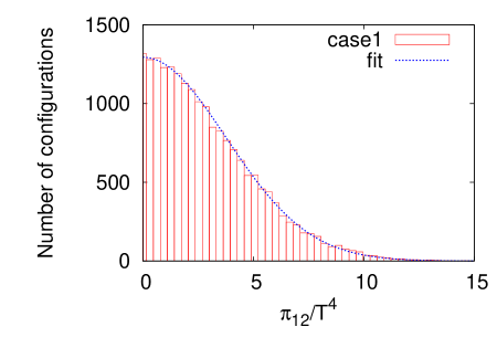
Figure 1: Distribution of fluctuation of $\bar{\pi}_{12}$ obtained from numerical simulations for case1. The horizontal axis is normalized by the temperature. The dotted line denotes the Gaussian fit.

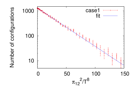
Figure 2: Distribution of ${\pi_{12}}^{2}$ obtained from numerical simulations for case 1. The vertical axis is logarithmic. $\beta_{2}$ can be read from the gradient of fit line.

In this work, we perform the lattice simulation for SU(3) pure gauge theory with the standard Wilson gauge action. Configurations are generated by heatbath and overrelaxation algorithms. In Table 1 we show lattice parameters used in this work. The simulation is performed with three lattice sizes $N_{\sigma}^{3}\times N_{\tau}$ with a periodic boundary condition and different lattice spacing $a$. For each parameter, 10000 configurations have been prepared. The energy momentum tensor is given by $T^{\mu\nu}=2{\rm tr}\left[F^{\mu}_{\rho}F^{\rho\nu}+(1/4)g^{\mu\nu}F^{\rho\sigma}F_{\rho\sigma}\right]$. For the definition of the field strength on the lattice, we have chosen the clover operator.

For the spatial average in Eq. (17), we take the average of $T_{\mu\nu}$ on a cube of size $(N_{\sigma}/2)^{3}$ to remove the effect of periodicity. For each configuration one can take eight such subconfigurations on cubes. We regard two of the cubes aligned in a diagonal direction as statistically independent areas. Furthermore, we adopt two sets of subconfigurations on the two time slices at $N_{\tau}=0$ and $N_{\tau}=1/2aT$ in order to improve statistics. In this way, four subconfigurations are taken from each configuration for analysis.

In Fig. 1, we show the distribution of the spatial average of the shear viscous pressure $\bar{\pi}_{12}=\bar{T}_{12}$ for case 1. The same result is shown in Fig. 2 with different choices of vertical and horizontal axes. These figures show that the distribution of $\bar{\pi}_{12}$ is of Gaussian form, as anticipated. Extracting fluctuations from this distribution and substituting the result to Eq. (19), we obtain

$$\beta_{2}\simeq 0.0036.$$ (23)

This value of $\beta_{2}$ is, however, quite small in the sense that the relaxation time $\tau_{\pi}=2\beta_{2}\eta$ is so small for $\eta\lesssim 1$ that IS theory turns back to the first order theory. In fact, the speed of transverse plane wave, $v_{T}$, with the value of $\beta_{2}$ in Eq. (23) gives [11]

$$\frac{v_{T}}{c}=\sqrt{\frac{1}{2\beta_{2}(\epsilon+p)}}\simeq 6,$$ (24)

where we have used the values of $\epsilon$ and $p$ obtained in the previous work on bulk thermodynamics of SU(3) gauge theory [13]. Eq. (24) means that causality is violated with $\beta_{2}$ obtained in this analysis. Similar results are obtained on cases 2 and 3.

6 Discussions

In this work, we tried to evaluate the ratio between the relaxation time $\tau_{\pi}$ and the shear viscosity $\eta$ in SU(3) gauge theory by lattice simulations. Using BE principle and the form of entropy in IS theory, the ratio is related to statistical fluctuation of stress tensor in equilibrium through Eq. (19). In the numerical simulations, however, we have observed large fluctuations of stress tensor, $\langle\bar{\pi}_{12}^{2}\rangle$, which leads to unacceptably small $\beta_{2}$ violating causality.

It is, however, suspicious to simply apply fluctuations obtained on the lattice to Eq. (19), since $\langle\bar{\pi}_{12}^{2}\rangle$ is actually an ultraviolet divergent quantity and it diverges even in the vacuum. The large fluctuations would have originated from this vacuum fluctuations, which should be subtracted to obtain the physical value of fluctuations. This analysis is in progress. The present numerical results, however, indicate that we need more statistics to separate physical fluctuations from the vacuum one with a good accuracy.

References

- [1] C. Eckart, Phys. Rev. 58 (1940) 919.
- [2] L.D. Landau and E.M. Lifshitz, fluid mechanics (Pergamon, New York, 1959).
- [3] W. A. Hiscock and L. Lindblom, Annals Phys. 151 (1983) 466.
- [4] W. Israel and J. M. Stewart, Annals Phys. 118 (1979) 341.
- [5] P. Arnold, G. D. Moore and L. G. Yaffe, JHEP 0011 (2000) 001 [arXiv:hep-ph/0010177].
- [6] F. Karsch and H. W. Wyld, Phys. Rev. D 35 (1987) 2518.
- [7] A. Nakamura and S. Sakai, Phys. Rev. Lett. 94 (2005) 072305 [arXiv:hep-lat/0406009].
- [8] H. B. Meyer, arXiv:0907.4095 [hep-lat].
- [9] A. Muronga, Eur. Phys. J. ST 155 (2008) 107 [arXiv:0710.3280 [nucl-th]].
- [10] S. Pratt, Phys. Rev. C 77 (2008) 024910 [arXiv:0711.3911 [nucl-th]].
- [11] A. Muronga, Phys. Rev. C 69 (2004) 034903 [arXiv:nucl-th/0309055].
- [12] W. Israel, Annals Phys. 100 (1976) 310.
- [13] G. Boyd, et al., Nucl. Phys. B 469 (1996) 419 [arXiv:hep-lat/9602007]; M. Okamoto, et al. [CP-PACS Collaboration], Phys. Rev. D 60 (1999) 094510 [arXiv:hep-lat/9905005].