Adaptive–Wave Alternative for
the Black–Scholes Option Pricing Model

Abstract

A nonlinear wave alternative for the standard Black–Scholes option–pricing model is presented. The adaptive-wave model, representing controlled Brownian behavior of financial markets, is formally defined by adaptive nonlinear Schrödinger (NLS) equations, defining the option-pricing wave function in terms of the stock price and time. The model includes two parameters: volatility (playing the role of dispersion frequency coefficient), which can be either fixed or stochastic, and adaptive market potential that depends on the interest rate. The wave function represents quantum probability amplitude, whose absolute square is probability density function. Four types of analytical solutions of the NLS equation are provided in terms of Jacobi elliptic functions, all starting from de Broglie’s plane-wave packet associated with the free quantum-mechanical particle. The best agreement with the Black–Scholes model shows the adaptive shock-wave NLS-solution, which can be efficiently combined with adaptive solitary-wave NLS-solution. Adjustable ‘weights’ of the adaptive market-heat potential are estimated using either unsupervised Hebbian learning, or supervised Levenberg–Marquardt algorithm. In the case of stochastic volatility, it is itself represented by the wave function, so we come to the so-called Manakov system of two coupled NLS equations (that admits closed-form solutions), with the common adaptive market potential, which defines a bidirectional spatio-temporal associative memory.

Keywords: Black–Scholes option pricing, adaptive nonlinear Schrödinger equation,
market heat potential, controlled stochastic volatility, adaptive Manakov system,
controlled Brownian behavior

1 Introduction

The celebrated Black–Scholes partial differential equation (PDE) describes the time–evolution of the market value of a stock option [1, 2]. Formally, for a function $u=u(t,s)$ defined on the domain $0\leq s<\infty,~{}0\leq t\leq T$ and describing the market value of a stock option with the stock (asset) price $s$, the Black–Scholes PDE can be written (using the physicist notation: $\partial_{z}u=\partial u/\partial z$) as a diffusion–type equation:

$$\partial_{t}u=-\frac{1}{2}(\sigma s)^{2}\,\partial_{ss}u-rs\,\partial_{s}u+ru,$$ (1)

where $\sigma>0$ is the standard deviation, or volatility of $s$, $r$ is the short–term prevailing continuously–compounded risk–free interest rate, and $T>0$ is the time to maturity of the stock option. In this formulation it is assumed that the underlying (typically the stock) follows a geometric Brownian motion with ‘drift’ $\mu$ and volatility $\sigma$, given by the stochastic differential equation (SDE) [5]

$$ds(t)=\mu s(t)dt+\sigma s(t)dW(t),$$ (2)

where $W$ is the standard Wiener process.

The economic ideas behind the Black–Scholes option pricing theory translated to the stochastic methods and concepts are as follows (see [6]). First, the option price depends on the stock price and this is a random variable evolving with time. Second, the efficient market hypothesis [7, 8], i.e., the market incorporates instantaneously any information concerning future market evolution, implies that the random term in the stochastic equation must be delta–correlated. That is: speculative prices are driven by white noise. It is known that any white noise can be written as a combination of the derivative of the Wiener process [39] and white shot noise (see [9]). In this framework, the Black–Scholes option pricing method was first based on the geometric Brownian motion [1, 2], and it was lately extended to include white shot noise.

The Black-Sholes PDE (1) is usually derived from SDEs describing the geometric Brownian motion (2), with the stock-price solution given by:

$$s(t)=s(0)\mathrm{e}^{(\mu-\frac{1}{2}\sigma^{2})t+\sigma W(t)}.$$

In mathematical finance, derivation is usually performed using Itô lemma [37] (assuming that the underlying asset obeys the Itô SDE), while in physics it is performed using Stratonovich interpretation (assuming that the underlying asset obeys the Stratonovich SDE [38]) [9, 6].

The PDE (1) resembles the backward Fokker–Planck equation (also known as the Kolmogorov forward equation, in which the probabilities diffuse outwards as time moves forwards) describes the time evolution of the probability density function $p=p(t,x)$ for the position $x$ of a particle, and can be generalized to other observables as well [3]. Its first use was statistical description of Brownian motion of a particle in a fluid. Applied to the option–pricing process $p=p(t,s)$ with drift $D_{1}=D_{1}(t,s)$, diffusion $D_{2}=D_{2}(t,s)$ and volatility $\sigma^{2}$, the forward Fokker–Planck equation reads:

$$\partial_{t}p=\frac{1}{2}\partial_{ss}\left(D_{2}\sigma^{2}p\right)-\partial_{s}\left(D_{1}p\right).$$

The corresponding backward Fokker–Planck equation (which is probabilistic diffusion in reverse, i.e., starting at the final forecasts, the probabilities diffuse outwards as time moves backwards) reads:

$$\partial_{t}p=-\frac{1}{2}\sigma^{2}\partial_{ss}\left(D_{2}p\right)-\partial_{s}\left(D_{1}p\right).$$

The solution of the PDE (1) depends on boundary conditions, subject to a number of interpretations, some requiring minor transformations of the basic BS equation or its solution.

The basic equation (1) can be applied to a number of one-dimensional models of interpretations of prices given to $u$, e.g., puts or calls, and to $s$, e.g., stocks or futures, dividends, etc. The most important examples are European call and put options (see Figure 1), defined by:

$$u_{\mathrm{Call}}(s,t)=s\,\mathcal{N}(\mathrm{d_{1}})\,\mathrm{e}^{-T\delta}-k\,\mathcal{N}(\mathrm{d_{2}})\,\mathrm{e}^{-rT},$$ (3)

$$u_{\mathrm{Put}}(s,t)=k\,\mathcal{N}(-\mathrm{d_{2}})\,\mathrm{e}^{-rT}-s\,\mathcal{N}(-\mathrm{d_{1}})\,\mathrm{e}^{-T\delta},$$ (4)

$$\,\mathcal{N}(\lambda)=\frac{1}{2}\left(1+\mathrm{erf}\left(\frac{\lambda}{\sqrt{2}}\right)\right),$$

$$\mathrm{d_{1}}=\frac{\ln\left(\frac{s}{k}\right)+T\left(r-\delta+\frac{\sigma^{2}}{2}\right)}{\sigma\sqrt{T}},\qquad\mathrm{d_{2}}=\frac{\ln\left(\frac{s}{k}\right)+T\left(r-\delta-\frac{\sigma^{2}}{2}\right)}{\sigma\sqrt{T}},$$

where erf$(\lambda)$ is the (real-valued) error function, $k$ denotes the strike price and $\delta$ represents the dividend yield. In addition, for each of the call and put options, there are five Greeks (see, e.g. [22]), or sensitivities of the option-price with respect to the following quantities:

1. The stock price – Delta: $\Delta_{\mathrm{Call}}=\partial_{s}u_{\mathrm{Call}}\$and $\Delta_{\mathrm{Put}}=\partial_{s}u_{\mathrm{Put}};$

2. The interest rate – Rho: $\rho_{\mathrm{Call}}=\partial_{r}u_{\mathrm{Call}}\$and $\rho_{\mathrm{Put}}=\partial_{r}u_{\mathrm{Put}};$

3. The volatility: Vega${}_{\mathrm{Call}}=\partial_{\sigma}u_{\mathrm{Call}}\$and Vega${}_{\mathrm{Put}}=\partial_{\sigma}u_{\mathrm{Put}};$

4. The elapsed time since entering into the option – Theta:
   $\Theta_{\mathrm{Call}}=\partial_{T}u_{\mathrm{Call}}\$and $\Theta_{\mathrm{Put}}=\partial_{T}u_{\mathrm{Put}};$  and

5. The second partial derivative of the option-price with respect to the stock price – Gamma: $\Gamma_{\mathrm{Call}}=\partial_{ss}u_{\mathrm{Call}}\$and $\Gamma_{\mathrm{Put}}=\partial_{ss}u_{\mathrm{Put}}$.

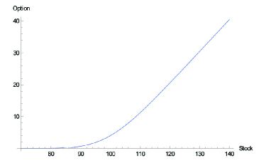
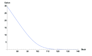
Figure 1: European call (3) and put (4) options, as the solutions of the Black-Sholes PDE (1). Used parameters are: $\sigma=0.3,\,r=0.05,\,k=100,\,\delta=0.04$ [22].

In practice, the volatility $\sigma$ is the least known parameter in (1), and its estimation is generally the most important part of pricing options. Usually, the volatility is given in a yearly basis, baselined to some standard, e.g., 252 trading days per year, or 360 or 365 calendar days. However, and especially after the 1987 crash, the geometric Brownian motion model and the BS formula were unable to reproduce the option price data of real markets.

The Black–Scholes model assumes that the underlying volatility is constant over the life of the derivative, and unaffected by the changes in the price level of the underlying. However, this model cannot explain long-observed features of the implied volatility surface such as volatility smile and skew, which indicate that implied volatility does tend to vary with respect to strike price and expiration. By assuming that the volatility of the underlying price is a stochastic process itself, rather than a constant, it becomes possible to model derivatives more accurately.

As an alternative, models of financial dynamics based on two-dimensional diffusion processes, known as stochastic volatility (SV) models [10], are being widely accepted as a reasonable explanation for many empirical observations collected under the name of ‘stylized facts’ [11]. In such models the volatility, that is, the standard deviation of returns, originally thought to be a constant, is a random process coupled with the return in a SDE of the form similar to (2), so that they both form a two-dimensional diffusion process governed by a pair of Langevin equations [10, 12, 13].

Using the standard Kolmogorov probability approach, instead of the market value of an option given by the Black–Scholes equation (1), we could consider the corresponding probability density function (PDF) given by the backward Fokker–Planck equation (see [9]). Alternatively, we can obtain the same PDF (for the market value of a stock option), using the quantum–probability formalism [44, 45], as a solution to a time–dependent linear Schrödinger equation for the evolution of the complex–valued wave $\psi-$function for which the absolute square, $|\psi|^{2},$ is the PDF (see [48]).

In this paper, I will go a step further and propose a novel general quantum–probability based, option–pricing model, which is both nonlinear (see [16, 17, 18, 20]) and adaptive (see [21, 19, 4, 40]). More precisely, I propose a quantum neural computation [32] approach to option price modelling, based on the nonlinear Schrödinger (NLS) equation with adaptive parameters.

2 Adaptive nonlinear Schrödinger equation model

This new adaptive wave–form approach to financial modelling is motivated by:

1. Modern adaptive markets hypothesis of A. Lo [49, 50];

2. My adaptive path integral approach to human cognition [29, 30, 31];

3. Elliott wave (fractal) market theory [51, 52, 53];  and

4. My recent monograph: ‘Quantum Neural Computation’ [32], as well as papers on entropic crowd modelling based on the concept of controlled Brownian motion [33, 34, 35].

To satisfy both efficient and behavioral markets, as well as their essential nonlinear complexity, I propose an adaptive, wave–form, nonlinear and stochastic option–pricing model with stock price $s,$ volatility $\sigma$ and interest rate $r$. The model is formally defined as a complex-valued, focusing (1+1)–NLS equation, defining the option–price wave function $\psi=\psi(s,t)$, whose absolute square $|\psi(s,t)|^{2}$ represents the probability density function (PDF) for the option price in terms of the stock price and time. In natural quantum units, this NLS equation reads:

$$\mathrm{i}\partial_{t}\psi=-\frac{1}{2}\sigma\partial_{ss}\psi-\beta|\psi|^{2}\psi,\qquad(\mathrm{i}=\sqrt{-1})$$ (5)

where dispersion frequency coefficient $\sigma$ is the volatility (which can be either constant or stochastic process itself), while Landau coefficient $\beta=\beta(r,w)$ represents the adaptive market potential, which is, in the simplest nonadaptive scenario, equal to the interest rate $r$, while in the adaptive case depends on the set of adjustable parameters $\{w_{i}\}$. In this case, $\beta(r,w)$ can be related to the market temperature (which obeys Boltzman distribution [15]). The term $V(\psi)=-\beta|\psi|^{2}$ represents the $\psi-$dependent potential field. Physically, the NLS equation (5) describes a nonlinear wave–packet defined by the complex-valued wave function $\psi(s,t)$ of real space and time parameters. In the present context, the space-like variable $s$ denotes the stock (asset) price.

2.1 Analytical NLS–solution

NLS equation can be exactly solved using the power series expansion method [54, 55] of Jacobi elliptic functions [56].

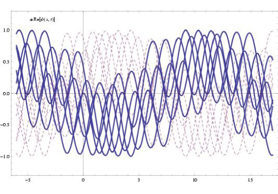
Figure 2: The general Jacobi sine solution (12) of the NLS equation (5) with $k=1.2,\,m=0.5$, $\sigma=\beta=1$, for $t\in(0,5)$ and $s\in(-7,18)$. Thick line represents +Re$[\psi(s,t)]$, while dash line represents –Re$[\psi(s,t)]$.

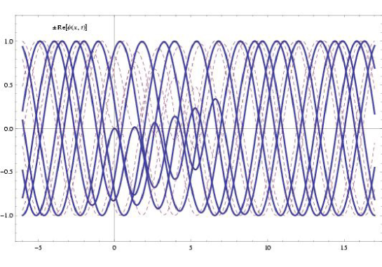
Figure 3: The dark shock-wave solution (13) of the NLS equation (5) with $k=1.2$, $\sigma=\beta=1$, for $t\in(0,5)$ and $s\in(-7,18)$. Thick line represents +Re$[\psi(s,t)]$, while dash line represents –Re$[\psi(s,t)]$.

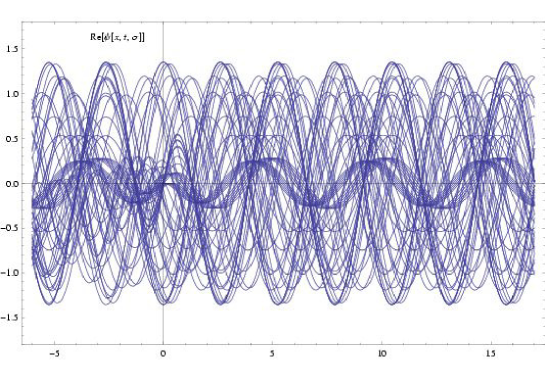
Figure 4: The +tanh solution from Figure 3, with stochastic volatility $\sigma_{t}$ (random walk).

In case of $\beta\ll 1$, $V(\psi)\rightarrow 0$, so equation (5) can be approximated by a linear wave packet, defined by a continuous superposition of de Broglie’s plane waves, associated with a free quantum particle. This linear wave packet is defined by the simple linear Schrödinger equation with zero potential energy (in natural units):

$$\mathrm{i}\partial_{t}\psi=-\frac{1}{2}\partial_{ss}\psi.$$ (6)

Thus, we consider the $\psi-$function describing a single de Broglie’s plane wave, with the wave number (or, momentum) $k$ and circular frequency $\omega$:

$$\psi(s,t)=\phi(\xi)\,\mathrm{e}^{\mathrm{i}(ks-\omega t)},\qquad\text{with \ }\xi=s-\sigma kt\text{ \ and \ }\phi(\xi)\in\mathbb{R}.$$ (7)

Its substitution into the linear Schrödinger equation (6) gives the linear harmonic oscillator ODE, whose eigenvalues are natural frequencies of (6) and the solution is given by a Fourier sine or cosine series (see, e.g. [57, 58]).

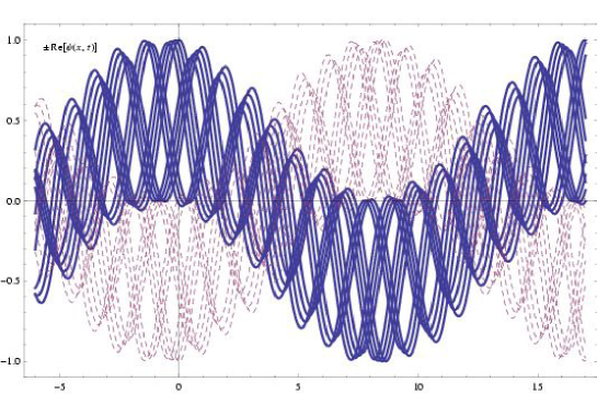
Figure 5: The general Jacobi cosine solution (14) of the NLS equation (5) with $k=1.2,\,m=0.5$, $\sigma=\beta=1$, for $t\in(0,10)$ and $s\in(-7,18)$. Thick line represents +Re$[\psi(s,t)]$, while dash line represents –Re$[\psi(s,t)]$.

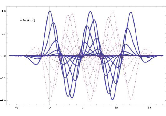
Figure 6: The bright solitary-wave solution (15) of the NLS equation (5) with $k=1.2$, $\sigma=\beta=1$, for $t\in(0,10)$ and $s\in(-7,18)$. Thick line represents +Re$[\psi(s,t)]$, while dash line represents –Re$[\psi(s,t)]$.

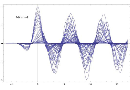
Figure 7: The +sech soliton from Figure 6, with stochastic volatility $\sigma_{t}$ (random walk).

Similarly, substituting (7) into the NLS equation (5), we obtain a nonlinear oscillator ODE:

$$\phi^{\prime\prime}(\xi)+[\omega-\frac{1}{2}\sigma k^{2}]\,\phi(\xi)+\beta\phi^{3}(\xi)=0.$$ (8)

Following [55], I suppose that a solution $\phi(\xi)$ for (8) can be obtained as a linear expansion

$$\phi(\xi)=a_{0}+a_{1}\mathrm{sn}(\xi),$$ (9)

where $\mathrm{sn}(s)=\mathrm{sn}(s,m)$ are Jacobi elliptic sine functions with elliptic modulus $m\in[0,1]$, such that $\mathrm{sn}(s,0)=\sin(s)\$and $\mathrm{sn}(s,1)=\mathrm{\tanh}(s)$. Using standard identities with associated elliptic cosine functions $\mathrm{cn}(\xi)$ and elliptic functions of the third kind $\mathrm{dn}(\xi)$, we have

$$\phi^{\prime}(\xi) = a_{1}\mathrm{cn}(\xi)\,\mathrm{dn}(\xi),$$

$$\phi^{\prime\prime}(\xi) = -a1\{\mathrm{sn}(\xi)[1-m^{2}\mathrm{sn}^{2}(\xi)]+m^{2}\mathrm{sn}(\xi)[1-\mathrm{sn}^{2}(\xi)]\}.$$ (10)

Substituting (9) and (10) into (8), after doing some algebra, we get

$$a_{0}=0,\qquad a_{1}=\pm m\sqrt{\frac{-\sigma}{\beta}},\qquad\omega=\frac{1}{2}(1+m^{2}+k^{2}),$$ (11)

which, substituted into the nonlinear oscillator (8), gives

$$\phi(\xi) = \pm m\sqrt{\frac{-\sigma}{\beta}}\,\mathrm{sn}(\xi),\qquad~{}\text{for~{}~{}}m\in[0,1];~{}~{}\text{and}$$

$$\phi(\xi) = \pm\sqrt{\frac{-\sigma}{\beta}}\,\mathrm{\tanh}(\xi),\qquad\text{for~{}~{}}m=1.$$

Using the substitutions (7) and (11), we now obtain the exact periodic solution of (5) as

$$\psi_{1}(s,t) = \pm m\sqrt{\frac{-\sigma}{\beta(w)}}\,\mathrm{sn}(s-\sigma kt)\,\mathrm{e}^{\mathrm{i}[ks-\frac{1}{2}\sigma t(1+m^{2}+k^{2})]},\qquad~{}~{}\text{for~{}~{}}m\in[0,1);$$ (12)

$$\psi_{2}(s,t) = \pm\sqrt{\frac{-\sigma}{\beta(w)}}\,\mathrm{\tanh}(s-\sigma kt)\,\mathrm{e}^{\mathrm{i}[ks-\frac{1}{2}\sigma t(2+k^{2})]},\qquad\qquad\text{for~{}~{}}m=1,$$ (13)

where (12) defines the general solution (see Figure 2), while (13) defines the envelope shock-wave (or, ‘dark soliton’) solution (Figure 3) of the NLS equation (5). The same shock-wave solution with stochastic volatility $\sigma_{t}$ (defined as a simple random walk) is given in Figure 4.

Alternatively, if we seek a solution $\phi(\xi)$ as a linear expansion of Jacobi elliptic cosine functions, such that $\mathrm{cn}(s,0)=\cos(s)$ and $\mathrm{cn}(s,1)=\mathrm{sech}(s)$, in a linear form:

$$\phi(\xi)=a_{0}+a_{1}\mathrm{cn}(\xi),$$

then we get

$$\psi_{3}(s,t) = \pm m\sqrt{\frac{\sigma}{\beta(w)}}\,\mathrm{cn}(s-\sigma kt)\,\mathrm{e}^{\mathrm{i}[ks-\frac{1}{2}\sigma t(1-2m^{2}+k^{2})]},\qquad\text{for~{}~{}}m\in[0,1);$$ (14)

$$\psi_{4}(s,t) = \pm\sqrt{\frac{\sigma}{\beta(w)}}\,\mathrm{sech}(s-\sigma kt)\,\mathrm{e}^{\mathrm{i}[ks-\frac{1}{2}\sigma t(k^{2}-1)]},\qquad\qquad\text{for~{}~{}}m=1,$$ (15)

where (14) defines the general solution (Figure 5), while (15) defines the envelope solitary-wave (or, ‘bright soliton’) solution (Figure 6) of the NLS equation (5). The same soliton solution with stochastic volatility $\sigma_{t}$ (a simple random walk) is given in Figure 4.

In all four solution expressions (12), (13), (14) and (15), the adaptive potential $\beta(w)$ is yet to be calculated using either unsupervised Hebbian learning, or supervised Levenberg–Marquardt algorithm (see, e.g. [41, 42]). In this way, the NLS equation (5) resembles the ‘quantum stochastic-filtering neural network’ model of [23, 24, 25]. While the authors of the prior quantum neural network performed only numerical (finite-difference) simulations of their model, this paper provides theoretical foundation (of both single NLS network and coupled NLS network) with closed-form analytical solutions. Any kind of numerical analysis can be easily performed using above closed-form solutions $\psi_{i}(s,t),~{}~{}(i=1,...,4)$.

2.2 Fitting the Black–Scholes model using adaptive NLS–PDF

The adaptive NLS–PDFs of the shock-wave type (13) can be used to fit the Black–Scholes call and put options. Specifically, I have used the spatial part of (13),

$$\phi(s)=\left|\sqrt{\frac{\sigma}{\beta}}\tanh(s-kt\sigma)\right|{}^{2},$$ (16)

where the adaptive market–heat potential $\beta(r,w)$ is chosen as:

$$\beta(r,w)=r\sum_{i=1}^{n}w_{1}^{i}\,\text{erf}\left(\frac{w_{2}^{i}s}{w_{3}^{i}}\right)$$ (17)

Figure 8: Fitting the Black–Scholes call option with $\beta(w)$-adaptive PDF of the shock-wave NLS-solution (13).

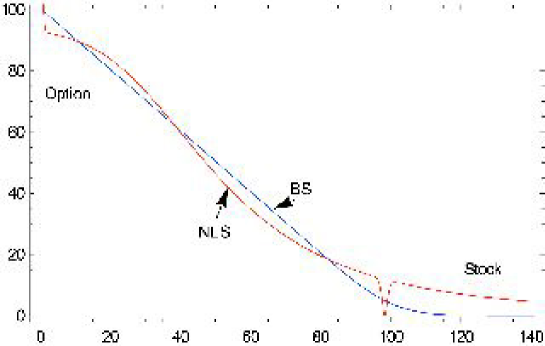
Figure 9: Fitting the Black–Scholes put option with $\beta(w)$ –adaptive PDF of the shock-wave NLS $\psi_{2}(s,t)$ solution (13). Notice the kink near $s=100$.

The following parameter estimates where obtained using 100 iterations of the Levenberg–Marquardt algorithm. In case of the call option fit (see Figure 8), $n=5$,

$w_{1}^{1}=24.8952,~{}w_{2}^{1}=-78112.3,~{}w_{3}^{1}=-48178.3,$

$w_{1}^{2}=24.8951,~{}w_{2}^{2}=-78112.3,~{}w_{3}^{2}=-48178.3,$

$w_{1}^{3}=24.895,~{}w_{2}^{3}=-78112.3,~{}w_{3}^{3}=-48178.3,$

$w_{1}^{4}=-37.3927,~{}w_{2}^{4}=-3108.08,~{}w_{3}^{4}=-1520633,$

$w_{1}^{5}=-37.2757,~{}w_{2}^{5}=-3968.35,~{}w_{3}^{5}=-159782.$

$\sigma^{\mathrm{call}}_{\mathrm{NLS}}=-0.119341\sigma_{\mathrm{BS}}$, $k^{\mathrm{call}}_{\mathrm{NLS}}=0.0156422k_{\mathrm{BS}}$, $T^{\mathrm{call}}_{\mathrm{NLS}}=15.6423T_{\mathrm{BS}}.$

In case of the put option fit (see Figure (9)), $n=3$,

$w_{a}^{1}=0.000222367,~{}w_{b}^{1}=82032.8,~{}w_{c}^{1}=63876.9,$

$w_{a}^{2}=-0.428113,~{}w_{b}^{2}=439.148,~{}w_{c}^{2}=205780.0,$

$w_{a}^{3}=4.70615,~{}w_{b}^{3}=27.1558,~{}w_{c}^{3}=139805.0$

$\sigma^{\mathrm{put}}_{\mathrm{NLS}}=-0.003444\sigma_{\mathrm{BS}}$, $k^{\mathrm{put}}_{\mathrm{NLS}}=-3.10354k_{\mathrm{BS}}$, $T^{\mathrm{put}}_{\mathrm{NLS}}=-3103.54T_{\mathrm{BS}}.$

As can be seen from Figure (9) there is a kink near $s=100$. This kink, which is a natural characteristic of the spatial shock-wave (16), can be smoothed out by taking the sum of the spatial parts of the shock-wave NLS-solution (13) and the soliton NLS-solution (15) as:

$$\phi(s)=\left|\sqrt{\frac{\sigma}{\beta}}\left[d_{1}\tanh(s-kt\sigma)+d_{2}\,\text{sech}(s-kt\sigma)\right]\right|{}^{2}.$$ (18)

In this case, using 100 iterations of the Levenberg–Marquardt algorithm, the following parameter estimates where obtained:

$w_{1}^{1}=-0.00190885,\,w_{2}^{1}=6798.78,\,w_{3}^{1}=5329.46,\,$

$w_{1}^{2}=18.1757,\,w_{2}^{2}=23.5253,\,w_{3}^{2}=18354.9,\,$

$w_{1}^{3}=-71.7315,\,w_{2}^{3}=4.15999,\,w_{3}^{3}=12807.2,\,$

$d_{1}=0.345078,\,d_{2}=-12.3948.$

$\sigma^{\mathrm{put}}_{\mathrm{NLS}}=-0.247932_{\mathrm{BS}},\,k^{\mathrm{put}}_{\mathrm{NLS}}=0.260764k_{\mathrm{BS}},\,T^{\mathrm{put}}_{\mathrm{NLS}}=260.764T_{\mathrm{BS}}.$

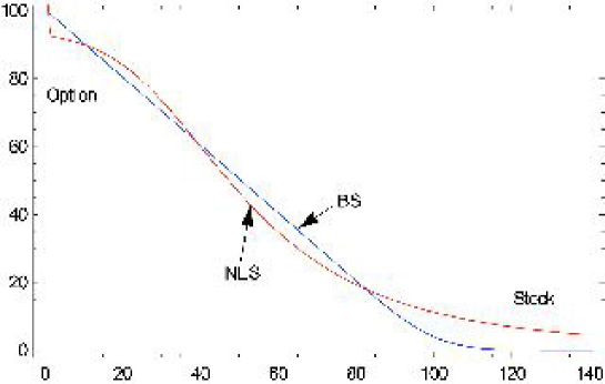
Figure 10: Smoothing out the kink in the put option fit, by combining the shock-wave solution with the soliton solution, as defined by (18).

The adaptive NLS–based Greeks can now be defined, using $\beta=r$ and above modified $(\sigma,\,k,\,t)$ values, by the following partial derivatives of the spatial part of the shock-wave solution (13):

$\mathrm{Delta}=\partial_{s}\phi(s)=2\sqrt{-\frac{\sigma}{r}}\sqrt{\left|\frac{\sigma}{r}\right|}\text{sech}^{2}(s-kt\sigma)|\tanh(s-kt\sigma)|\text{abs}^{\prime}\left(\sqrt{-\frac{\sigma}{r}}\tanh(s-kt\sigma)\right),$

$\mathrm{Gamma}=\partial_{s}s\phi(s)=-\frac{2\text{sech}^{4}(s-kt\sigma)}{r}[\sigma$abs${}^{\prime}\left(\sqrt{-\frac{\sigma}{r}}\tanh(s-kt\sigma)\right)^{2}$

$+~{}\sqrt{\left|\frac{\sigma}{r}\right|}|\tanh(s-kt\sigma)|\{\sigma$abs${}^{\prime\prime}\left(\sqrt{-\frac{\sigma}{r}}\tanh(s-kt\sigma)\right)$

$+~{}r\sqrt{-\frac{\sigma}{r}}\sinh(2s-2kt\sigma)$abs${}^{\prime}\left(\sqrt{-\frac{\sigma}{r}}\tanh(s-kt\sigma)\right)\}],$

$\mathrm{Vega}=\partial_{\sigma}\phi(s)=\frac{\sqrt{-\frac{\sigma}{r}}\sqrt{\left|\frac{\sigma}{r}\right|}|\tanh(s-kt\sigma)|\left(\tanh(s-kt\sigma)-2kt\sigma\text{sech}^{2}(s-kt\sigma)\right)\text{abs}^{\prime}\left(\sqrt{-\frac{\sigma}{r}}\tanh(s-kt\sigma)\right)}{\sigma},$

$\mathrm{Rho}=\partial_{r}\phi(s)=\frac{\left(-\frac{\sigma}{r}\right)^{3/2}\sqrt{\left|\frac{\sigma}{r}\right|}\tanh(s-kt\sigma)|\tanh(s-kt\sigma)|\text{abs}^{\prime}\left(\sqrt{-\frac{\sigma}{r}}\tanh(s-kt\sigma)\right)}{\sigma},$

$\mathrm{Theta}=\partial_{t}\phi(s)=2kr\left(-\frac{\sigma}{r}\right)^{3/2}\sqrt{\left|\frac{\sigma}{r}\right|}\text{sech}^{2}(s-kt\sigma)|\tanh(s-kt\sigma)|\text{abs}^{\prime}\left(\sqrt{-\frac{\sigma}{r}}\tanh(s-kt\sigma)\right),$

where $\text{abs}^{\prime}(z)$ denotes the partial derivative of the absolute value upon the corresponding variable $z$.

2.3 Coupled adaptive NLS–system for volatility + option-price evolution modelling

For the purpose of including a controlled stochastic volatility into the adaptive–wave model (5), the full bidirectional quantum neural computation model for option price forecasting can be represented as a self-organized system of two coupled self-focusing NLS equations: one defining the option–price wave function $\psi=\psi(s,t)$ and the other defining the volatility wave function $\sigma=\sigma(s,t)$. The two NLS equations are coupled so that the volatility $\sigma$ is a parameter in the option–price NLS, while the option–price $\psi$ is a parameter in the volatility NLS. In addition, both processes evolve in a common self–organizing market heat potential, so they effectively represent an adaptively controlled Brownian behavior of a hypothetical financial market.

Formally, I here propose an adaptive, symmetrically coupled, volatility + option–pricing model (with interest rate $r$ and Hebbian learning rate $c$), which represents a bidirectional spatio-temporal associative memory. The model is defined by the following coupled–NLS+Hebb system:

$$\text{Volatility NLS :}\quad\mathrm{i}\partial_{t}\sigma = -\frac{1}{2}\partial_{ss}\mathcal{\sigma}-\beta\left(|\mathcal{\sigma}|^{2}+|\psi|^{2}\right)\mathcal{\sigma},$$ (19)

$$\text{Option price NLS :}\quad\mathrm{i}\partial_{t}\psi = -\frac{1}{2}\partial_{ss}\psi-\beta\left(|\mathcal{\sigma}|^{2}+|\psi|^{2}\right)\psi,$$ (20)

$$\text{with :}~{}~{}\beta(r,w) = r\sum_{i=1}^{N}w_{i}g_{i},\qquad\text{and}$$

$$\text{Adaptation ODE :}\quad\dot{w}_{i} = -w_{i}+c|\sigma|g_{i}|\psi|.$$ (21)

In this coupled model, the $\sigma$–NLS (19) governs the $(s,t)-$evolution of stochastic volatility, which plays the role of a nonlinear coefficient in (20); the $\psi$–NLS (20) defines the $(s,t)-$evolution of option price, which plays the role of a nonlinear coefficient in (19). The purpose of this coupling is to generate a leverage effect, i.e. stock volatility is (negatively) correlated to stock returns (see, e.g. [14]). The $w-$ODE (21) defines the $(\sigma,\psi)-$coupling based continuous Hebbian learning with the learning rate $c.$ The adaptive market–heat potential $\beta(r,w)$, previously defined by (17), is now generalized into a scalar product of the ‘synaptic weight’ vector $w_{i}$ and the Gaussian kernel vector $g_{i}$, yet to be defined.

The bidirectional associative memory model (19)–(20)–(21) effectively performs quantum neural computation [32], by giving a spatio-temporal and quantum generalization of Kosko’s BAM family of neural networks [26, 27]. In addition, the shock-wave and solitary-wave nature of the coupled NLS equations may describe brain-like effects frequently occurring in financial markets: volatility/price propagation, reflection and collision of shock and solitary waves (see [28]).

The coupled NLS-system (19)–(20), without an embedded $w-$learning (i.e., for constant $\beta=r$ – the interest rate), actually defines the well-known Manakov system, which was proven by S. Manakov in 1973 [59] to be completely integrable, by the existence of infinite number of involutive integrals of motion. It admits ‘bright’ and ‘dark’ soliton solutions. Manakov system has been used to describe the interaction between wave packets in dispersive conservative media, and also the interaction between orthogonally polarized components in nonlinear optical fibres (see, e.g. [61, 62] and references therein).

The simplest solution of (19)–(20), the so-called Manakov bright 2–soliton, has the form resembling that of (15) and (Figure 6) (see [63, 64, 65, 66, 67, 68, 69]), defined by:

$$\mathbf{\psi}_{\mathrm{sol}}(s,t)=2b\,\mathbf{c\,}\mathrm{sech}(2b(s+4at))\,\mathrm{e}^{-2\mathrm{i}(2a^{2}t+as-2b^{2}t)},$$ (22)

where $\mathbf{\psi}_{\mathrm{sol}}(s,t)=\left(\begin{array}[]{c}\sigma(s,t)\\ \psi(s,t)\end{array}\right)$, $\mathbf{c}=(c_{1},c_{2})^{T}$ is a unit vector such that $|c_{1}|^{2}+|c_{2}|^{2}=1$. Real-valued parameters $a$ and $b$ are some simple functions of $(\sigma,\beta,k)$, which can be determined by either Hebbian learning of Levenberg–Marquardt algorithm. Also, shock-wave solutions similar to (13) are derived in Appendix. We can argue that in some short-time financial situations, the adaptation effect (21) can be neglected, so our option-pricing model (19)–(20) can be reduced to the Manakov 2–soliton model (22), as depicted and explained in Figure 11.

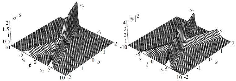
Figure 11: Hypothetical market scenario including sample PDFs for volatility $|\mathcal{\sigma}|^{2}$ and $|\psi|^{2}$ of the Manakov 2–soliton (22). On the left, we observe the $(s,t)-$evolution of stochastic volatility: we have a collision of two volatility component-solitons, $S_{1}(s,t)$ and $S_{2}(s,t)$, which join together into the resulting soliton $S_{2}(s,t)$, annihilating the $S_{1}(s,t)$ component in the process. On the right, we observe the $(s,t)-$evolution of option price: we have a collision of two option component-solitons, $S_{1}(s,t)$ and $S_{2}(s,t)$, which pass through each other without much change, except at the collision point. Due to symmetry of the Manakov system, volatility and option price can exchange their roles.

More complex exact soliton solutions have been derived for the Manakov system (19)–(20) with different procedures (see Appendix, as well as [71, 72, 73]). For example, in [71], using bright one-soliton solutions (of the type of (15)) of the system (19)–(20), many physical phenomena, such as unstable birefringence property, soliton trapping and daughter wave (’shadow’) formation, were studied. Similarly, searching for modulation instabilities and homoclinic orbits was performed in [74, 76, 77]. In particular, local bifurcations of ‘wave and daughter waves’ from single-component waves have been studied in various forms of coupled NLS–systems, including the Manakov system (see [78] and references therein). Let us assume that a small volatility $\sigma-$component bifurcates from a pure option-price $\psi-$pulse. Thus, at the bifurcation point, the volatility component is infinitesimally small, while the option-price component is governed by the equation

$$\partial_{ss}\psi-\psi+\psi^{3}=0,$$

whose homoclinic soliton solution is

$$\psi(s)=\sqrt{2}\,\mbox{sech}\,s.$$ (23)

A necessary condition for a local bifurcation of a homoclinic soliton solution with a small-amplitude volatility component from the option-price pulse (23) is that there is a non-trivial localized solution to the linearized problem of the $\sigma-$component. This takes the form of a linear Schrödinger equation

$$\partial_{ss}\sigma-\omega^{2}\sigma+2\mbox{sech}^{2}s\,\sigma=0,$$ (24)

which can be solved exactly (see [80]), and for local bifurcation we require $\sigma\rightarrow 0~{}~{}\mbox{as}~{}~{}|s|\rightarrow\pm\infty.$

As a final remark, numerical solution of the adaptive Manakov system (19)–(20)–(21), with any possible extensions, is quite straightforward, using the powerful numerical method of lines (see Appendix in [32]). Another possibility is Berger-Oliger adaptive mesh refinement when recursively numerically solving partial differential equations with wave-like solutions, using characteristic (double-null) grids (see [79] and reference therein).

2.4 Hebbian learning dynamics: analytical solution

Regarding the Hebbian learning (21) embedded into the Manakov system (19)–(20), suppose e.g. that we have $N=10$ synaptic weights (in a single neural layer), with the learning rate $c=0.7$. The zero-mean Gaussians are defined as:

$$g_{i}=\mathrm{e}^{-~{}\frac{t^{2}}{2\sigma_{i}}},\qquad(i=1,...,N),$$

where $\{\sigma_{i}\}$ are $(-1,+1)-$random standard deviations. Using random initial conditions, we get (by Mathematica of Maple ODE-solvers) the following analytical solutions of the Hebbian learning ODEs:

$$\begin{array}[]{l}w_{1}(t)=\mathrm{e}^{-t}\left[136485~{}\text{erf}(0.686579(106069~{}t-1))~{}|\psi|^{2}+0.912318~{}|\psi|^{2}-0.00675663\right],\\ w_{2}(t)=\mathrm{e}^{-t}\left[0.932205~{}\text{erf}(0.553239(16336~{}t-1))~{}|\psi|^{2}+0.527646~{}|\psi|^{2}-0.249822\right],\\ w_{3}(t)=\mathrm{e}^{-t}\left[0.471627~{}\text{erfi}(0.477447(2.19341~{}t+1))~{}|\psi|^{2}-0.274787~{}|\psi|^{2}+0.582548\right],\\ w_{4}(t)=\mathrm{e}^{-t}\left[0.52899~{}\text{erfi}(0.6535(117079~{}t+1))~{}|\psi|^{2}-0.453506~{}|\psi|^{2}+0.0773187\right],\\ w_{5}(t)=\mathrm{e}^{-t}\left[0.362728~{}\text{erfi}(0.324902(4.73659~{}t+1))~{}|\psi|^{2}-0.137812~{}|\psi|^{2}+0.798481\right],\\ w_{6}(t)=\mathrm{e}^{-t}\left[0.523292~{}\text{erfi}(0.6177(131043~{}t+1))~{}|\psi|^{2}-0.416953~{}|\psi|^{2}-0.288671\right],\\ w_{7}(t)=\mathrm{e}^{-t}\left[0.692907~{}\text{erf}(0.454319(2.42241~{}t-1))~{}|\psi|^{2}+0.332217~{}|\psi|^{2}+0.761879\right],\\ w_{8}(t)=\mathrm{e}^{-t}\left[0.432141~{}\text{erf}(0.315332(5.02843~{}t-1))~{}|\psi|^{2}+0.148814~{}|\psi|^{2}-0.33264\right],\\ w_{9}(t)=\mathrm{e}^{-t}\left[0.530916~{}\text{erfi}(0.673709(11016~{}t+1))~{}|\psi|^{2}-0.473963~{}|\psi|^{2}-0.17079\right],\\ w_{10}(t)=\mathrm{e}^{-t}\left[0.443395~{}\text{erf}(0.322143(4.81806~{}t-1))~{}|\psi|^{2}+0.155768~{}|\psi|^{2}+0.49451\right],\end{array}$$

where $\text{erf}(s)$ denotes the real-valued error function, while $\text{erfi}(s)$ denotes the imaginary error function defined as: $\text{erf}(\mathrm{i}\,s)/\mathrm{i}$.

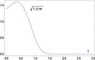
Figure 12: Time plot of the quick adaptive potential term $\sqrt{1/\beta(w)}$ (as it appears in $\psi_{i}(s,t),~{}~{}i=1,...,4$) for the sample value of $\psi(s,t)=0.5$.

In this way, we get the alternative expression for adaptive market–heat potential: $\beta(w)=r\sum_{i=1}^{N}w_{i}g_{i},$ with interest rate $r$ (see Figure 12). Insertion of $\beta(w)$, including the product $|\sigma(s,t)||\psi(s,t)|$ calculated at time $t$ into any Manakov solutions, gives the recursive QNN dynamics $\psi(s,t+1)$ for volatility and option-price forecasting at time $t+1$. For example, an instant snapshot of the adaptive bright sech-soliton $\psi_{4}(s,t)$ is given in Figure 13.

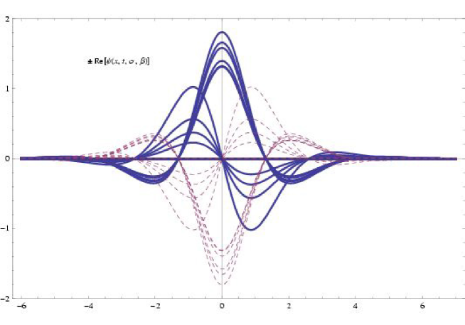
Figure 13: A snapshot of the adaptive $\pm$sech-soliton $\psi_{4}(s,t)$ with stochastic volatility $\sigma_{t}$ and trained potential $\beta(w)$ calculated at a sample fixed time $t_{0}$. We can see that due to quick learning dynamics, the whole solution is now decaying much faster than in Figure 6.

3 Conclusion

I have proposed a nonlinear adaptive–wave alternative to the standard Black-Scholes option pricing model. The new model, philosophically founded on adaptive markets hypothesis [49, 50] and Elliott wave market theory [51, 52], describes adaptively controlled Brownian market behavior, formally defined by adaptive NLS-equation. Four types of analytical solutions of the NLS equation are provided in terms of Jacobi elliptic functions, all starting from de Broglie’s plane waves associated with the free quantum-mechanical particle. The best agreement with the Black-Scholes model shows the adaptive shock-wave NLS-solution, which can be efficiently combined with adaptive solitary-wave NLS-solution. Adjustable ’weights’ of the adaptive market potential are estimated using either unsupervised Hebbian learning, or supervised Levenberg-Marquardt algorithm. For the case of stochastic volatility, it is itself represented by the wave function, so we come to the integrable Manakov system of two coupled NLS equations with the common adaptive potential, defining a bidirectional spatio-temporal associative memory machine.

As depicted in most Figures in this paper, the presented adaptive–wave model, both the single NLS-equation (5) and the coupled NLS-system (19)–(20)–(21), which represents a bidirectional associative memory, is a spatio-temporal dynamical system of great nonlinear complexity (see [40]), much more complex then the Black-Scholes model. This makes the new wave model harder to analyze, but at the same time, its immense variety is potentially much closer to the real financial market complexity, especially at the time of economic crisis abundant in shock-waves.

Finally, close in spirit to the adaptive–wave model is the method of adaptive wavelets in modern signal processing (see [81] and references therein, as well as [32] for an overview), which could be used for various market dimensionality reduction, signals separation and denoising as well as optimization of discriminatory market information.

4 Appendix: Manakov system

Manakov’s own method was based on the Lax pair representation. Alternatively, for normalized value of the market–heat potential, $\beta=r=1$, Manakov system allows solutions of the form:

$$\sigma(s,t)=\varphi(s)\,\mathrm{e}^{\mathrm{i}w_{\sigma}^{2}t},\qquad\psi(s,t)=\phi(s)\,\mathrm{e}^{\mathrm{i}w_{\psi}^{2}t},$$ (34)

where $\varphi$, $\phi$ are real-valued functions and $w_{\sigma},w_{\psi}$ are positive wave parameters for volatility and option-price. Substituting (34) into the Manakov equations we get the ODE-system [62]

$$\varphi^{\prime\prime}(s) = w_{\sigma}^{2}\varphi(s)-[\varphi^{2}(s)+\phi^{2}(s)]\,\varphi(s),$$ (35)

$$\phi^{\prime\prime}(s) = w_{\psi}^{2}\phi(s)-[\phi^{2}(s)+\varphi^{2}(s)]\,\phi(s).$$ (36)

For $w_{\sigma}=w_{\psi}=w$, equations (35)-(36) have a one-parameter family of symmetric single-humped soliton solutions (see the left part of Figure 14) given by

$$\varphi(s)=\pm\phi(s)=w\,\mathrm{sech}(w\,s),$$ (37)

as well as periodic solutions:

$$\varphi(s)=A\cos(Bs)\qquad\text{and}\qquad\phi(s)=A\sin(Bs),$$ (38)

where $A=\sqrt{w^{2}+B^{2}}$ (with $B$ an arbitrary parameter). For $0<w<1$ there is also another, in general asymmetric, one-parameter family of solutions for each fixed $w$ [62]

$$\varphi(s) = {\ }\sqrt{2(1-w^{2})}\cosh{(}ws{)}/{\kappa,}$$ (39)

$$\phi(s) = {\ -}w\sqrt{2(1-w^{2})}\sinh{(}s-s_{0}{)}/{\kappa},\qquad\text{where}$$

$$\kappa = \cosh(s)\cosh(w\,s)-w\sinh(s)\sinh(w\,s),$$

in which $\varphi$ is symmetric and $\phi$ antisymmetric.

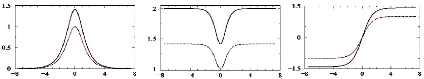
Figure 14: Initial envelopes for volatility $|\sigma_{0}|$ and option-price $|\psi_{0}|$ within the Manakov solitons: (left) bright compound soliton (37), (middle) dark compound soliton (40), and (right) compound kink-shaped soliton (44). These initial envelopes can be used for numerical studies of the Manakov system and its various generalizations (modified and adapted from [75]).

On the other hand, for negative values of the potential $\beta$, the Manakov equations accept dark soliton solutions of the form [75]

$$\sigma(s,t)=\psi(s,t)=k\left[\tanh(ks)-\mathrm{i}\right]\mathrm{e}^{\mathrm{i}(ks-5k^{2}t)},$$ (40)

which are localized dips on a finite-amplitude background wave (see the middle part of Figure 14). In this very interesting case, volatility and option-price fields are coupled together, forming a dark compound soliton. Note that their respective relative amplitudes are controlled by the corresponding nonlinearities and frequency. For $\beta=-1$ the Manakov equations alow also solutions of the form:

$$\sigma(s,t)=\varphi(s)\,\mathrm{e}^{-\mathrm{i}w_{\sigma}^{2}t},\qquad\,\,\psi(s,t)=\phi(s)\,\mathrm{e}^{-\mathrm{i}w_{\psi}^{2}t}.$$ (41)

Introducing (41) into the Manakov equations, we get the ODE-system:

$$\varphi^{\prime\prime}(s) = [\varphi^{2}(s)+\phi^{2}(s)]\,\varphi(s)-w_{\sigma}^{2}\varphi(s),$$ (42)

$$\phi^{\prime\prime}(s) = [\phi^{2}(s)+\varphi^{2}(s)]\,\phi(s)-w_{\psi}^{2}\phi(s),$$ (43)

which, for $w_{\sigma}=w_{\psi}=w$, allow for kink-shaped localized soliton solutions (see the right part of Figure 14) given by [75]

$$\varphi(s)=\pm\phi(s)=({w}/\sqrt{2})\tanh({w}\,s/\sqrt{2}),$$ (44)

as well as periodic solutions (38). Inserting (14) back into (41) gives the double-kink solution for the Manakov system:

$$\sigma(s,t)=\pm({w}/\sqrt{2})\tanh({w}\,s/\sqrt{2})\,\mathrm{e}^{-\mathrm{i}w^{2}t},\qquad\,\,\psi(s,t)=\pm({w}/\sqrt{2})\tanh({w}\,s/\sqrt{2})\mathrm{e}^{-\mathrm{i}w^{2}t}.$$ (45)

References

- [1] F. Black, M. Scholes, The Pricing of Options and Corporate Liabilities, J. Pol. Econ. 81, 637-659, (1973)
- [2] R.C. Merton, Theory of Rational Option Pricing, Bell J. Econ. and Management Sci. 4, 141-183, (1973)
- [3] L.P. Kadanoff, Statistical Physics: statics, dynamics and renormalization. World Scientific, Singapore, (2000)
- [4] V. Ivancevic, T. Ivancevic, Geometrical Dynamics of Complex Systems. Springer, Dordrecht, (2006)
- [5] M.F.M. Osborne, Brownian Motion in the Stock Market, Operations Research 7, 145-173, (1959)
- [6] J. Perello, J. M. Porra, M. Montero, J. Masoliver, Black-Scholes option pricing within Ito and Stratonovich conventions. Physica A 278, 1-2, 260-274, (2000)
- [7] E. Fama, The behavior of stock market prices. J. Business 38, 34-105, (1965)
- [8] M.C. Jensen, Some anomalous evidence regarding market efficiency, an editorial introduction, J. Finan. Econ. 6, 95-101, (1978)
- [9] C.W. Gardiner, Handbook of Stochastic Methods, Springer, Berlin, (1983)
- [10] J.P. Fouque, G. Papanicolau, and K. R. Sircar, Derivatives in Financial Markets with Stochastic Volatility. Cambdrige Univ. Press, Cambridge, (2000)
- [11] R. Cont, Empirical properties of asset returns: stylized facts and statistical issues. Quant. Finance 1, 223–236, (2001).
- [12] J. Perello, R. Sircar, J. Masoliver, Option pricing under stochastic volatility: the exponential Ornstein-Uhlenbeck model. J. Stat. Mech. P06010, (2008)
- [13] J. Masoliver, J. Perello, The escape problem under stochastic volatility: the Heston model. Phys. Rev. E 78, 056104, (2008)
- [14] H.E. Roman, M. Porto, C. Dose, Skewness, long-time memory, and non-stationarity: Application to leverage effect in financial time series. EPL 84, 28001, (5pp), (2008)
- [15] H. Kleinert, H. Kleinert, Path Integrals in Quantum Mechanics, Statistics, Polymer Physics, and Financial Markets (3rd ed), World Scientific, Singapore, (2002)
- [16] R.R. Trippi, Chaos & Nonlinear Dynamics in the Financial Markets. Irwin Prof. Pub. (1995)
- [17] P. Rothman, Nonlinear Time Series Analysis of Economic and Financial Data. Springer, (1999)
- [18] M. Ammann, C. Reich, VaR for nonlinear financial instruments – Linear approximation or full Monte-Carlo? Fin. Mark. Portf. Manag. 15(3), (2001)
- [19] L. Ingber, High-resolution path-integral development of financial options. Physica A 283, 529-558, (2000)
- [20] V. Ivancevic, T. Ivancevic, High-Dimensional Chaotic and Attractor Systems. Springer, Dordrecht, (2007)
- [21] W.M. Tse, Policy implications in an adaptive financial economy. J. Eco. Dyn. Con. 20(8), 1339-1366, 1996.
- [22] M. Kelly, Black-Scholes Option Model & European Option Greeks. The Wolfram Demonstrations Project, http://demonstrations.wolfram.com/EuropeanOptionGreeks, (2009)
- [23] L. Behera, I. Kar, Quantum Stochastic Filtering. In: Proc. IEEE Int. Conf. SMC 3, 2161–2167, (2005)
- [24] L. Behera, I. Kar, A.C. Elitzur, Recurrent Quantum Neural Network Model to Describe Eye Tracking of Moving Target, Found. Phys. Let. 18(4), 357-370, (2005)
- [25] L. Behera, I. Kar, A.C. Elitzur, Recurrent Quantum Neural Network and its Applications, Chapter 9 in The Emerging Physics of Consciousness, J.A. Tuszynski (ed.) Springer, Berlin, (2006)
- [26] B. Kosko, Bidirectional Associative Memory. IEEE Trans. Sys. Man Cyb. 18, 49–60, (1988)
- [27] B. Kosko, Neural Networks, Fuzzy Systems, A Dynamical Systems Approach to Machine Intelligence. Prentice–Hall, New York, (1992)
- [28] S.-H. Hanm, I.G. Koh, Stability of neural networks and solitons of field theory. Phys. Rev. E 60, 7608–7611, (1999)
- [29] V. Ivancevic, E. Aidman, Life-space foam: A medium for motivational and cognitive dynamics. Physica A 382, 616–630, (2007)
- [30] V. Ivancevic, T. Ivancevic, Nonlinear Quantum Neuro-Psycho-Dynamics with Topological Phase Transitions. NeuroQuantology 4, 349-368, (2008)
- [31] V. Ivancevic, E. Aidman, E., L. Yen, Extending Feynman’s Formalisms for Modelling Human Joint Action Coordination. Int. J. Biomath. 2(1), 1-7, (2009)
- [32] V. Ivancevic, T. Ivancevic, Quantum Neural Computation, Springer, (2009)
- [33] V. Ivancevic, D. Reid, Entropic Geometry of Crowd Dynamics. In Nonlinear Dynamics, Intech, Vienna, (in press)
- [34] V. Ivancevic, D. Reid, E. Aidman, Crowd Behavior Dynamics: Entropic Path-Integral Model. Nonlin. Dyn. (Springer, in press)
- [35] V. Ivancevic, D. Reid, Dynamics of Confined Crowds Modelled using Entropic Stochastic Resonance and Quantum Neural Networks. Int. J. Intel. Defence Sup. Sys. (in press)
- [36] F. Black, Studies of Stock Price Volatility Changes Proc. 1976 Meet. Ame. Stat. Assoc. Bus. Econ. Stat. 177—181, (1976)
- [37] K. Itô, On Stochastic Differential Equations, Mem. Am. Math. Soc. 4, 1-51, (1951)
- [38] R.L. Stratonovich, A new representation for stochastic integrals and equations. SIAM J. Control 4, 362-371, (1966)
- [39] N. Wiener, Differential space. J. Math. Phys. 2, 131–174, (1923)
- [40] V. Ivancevic, T. Ivancevic, Complex Nonlinearity: Chaos, Phase Transitions, Topology Change and Path Integrals, Springer, (2008)
- [41] V. Ivancevic, T. Ivancevic, Neuro-Fuzzy Associative Machinery for Comprehensive Brain and Cognition Modelling. Springer, Berlin, (2007)
- [42] V. Ivancevic, T. Ivancevic, Computational Mind: A Complex Dynamics Perspective. Springer, Berlin, (2007)
- [43] H. Spohn, Kinetic equations from Hamiltonian dynamics: Markovian limits. Rev. Mod. Phys. 52, 569–615, (1980)
- [44] V. Ivancevic, T. Ivancevic, Complex Dynamics: Advanced System Dynamics in Complex Variables. Springer, Dordrecht, (2007)
- [45] V. Ivancevic, T. Ivancevic, Quantum Leap: From Dirac and Feynman, Across the Universe, to Human Body and Mind. World Scientific, Singapore, (2008)
- [46] H. Umezawa, Advanced field theory: micro macro and thermal concepts. Am. Inst. Phys. New York, (1993)
- [47] W.J. Freeman, G. Vitiello, Nonlinear brain dynamics as macroscopic manifestation of underlying many–body field dynamics. Phys. Life Rev. 3(2), 93–118, (2006)
- [48] J. Voit, The Statistical Mechanics of Financial Markets. Springer, (2005)
- [49] A.W. Lo, The Adaptive Markets Hypothesis: Market Efficiency from an Evolutionary Perspective, J. Portf. Manag. 30, 15-29, (2004)
- [50] A.W. Lo, Reconciling Efficient Markets with Behavioral Finance: The Adaptive Markets Hypothesis, J. Inves. Consult. 7, 21-44, (2005)
- [51] A.J. Frost, R.R. Prechter, Jr., Elliott Wave Principle: Key to Market Behavior. Wiley, New York, (1978); (10th Edition) Elliott Wave International, (2009)
- [52] P. Steven, Applying Elliott Wave Theory Profitably. Wiley, New York, (2003)
- [53] B. Mandelbrot, A multifractal walk down Wall Street. Sci. Am. February (1999)
- [54] S. Liu, Z. Fu, S. Liu, Q. Zhao, Jacobi elliptic function expansion method and periodic wave solutions of nonlinear wave equations. Phys. Let. A 289, 69–74, (2001)
- [55] G-T. Liu, T-Y. Fan, New applications of developed Jacobi elliptic function expansion methods. Phys. Let. A 345, 161–166, (2005)
- [56] M. Abramowitz, I.A. Stegun, (Eds): Jacobian Elliptic Functions and Theta Functions. Chapter 16 in Handbook of Mathematical Functions with Formulas, Graphs, and Mathematical Tables (9th ed). Dover, New York, 567-581, (1972)
- [57] D.J. Griffiths, Introduction to Quantum Mechanics (2nd ed.), Pearson Educ. Int., (2005)
- [58] B. Thaller, Visual Quantum Mechanics, Springer, New York, (2000)
- [59] S.V. Manakov, On the theory of two-dimensional stationary self-focusing of electromagnetic waves. (in Russian) Zh. Eksp. Teor. Fiz. 65 505?516, (1973); (transleted into English) Sov. Phys. JETP 38, 248–253, (1974)
- [60] M. Lakshmanan, T. Kanna, R. Radhakrishnan, Shape-Changing Collisions of Coupled Bright Solitons in Birefringent Optical Fibers. Rep. Math. Phys. 46(1-2), 143-156, (2000)
- [61] M. Haelterman, A.P. Sheppard, Bifurcation phenomena and multiple soliton bound states in isotropic Kerr media. Phys. Rev. E 49, 3376?3381, (1994)
- [62] J. Yang, Classification of the solitary wave in coupled nonlinear Schrödinger equations. Physica D 108, 92?112, (1997)
- [63] D.J. Benney, A.C. Newell, The propagation of nonlinear wave envelops. J. Math. Phys. 46, 133-139, (1967)
- [64] V.E. Zakharov, S.V. Manakov, S.P. Novikov, L.P. Pitaevskii, Soliton theory: inverse scattering method. Nauka, Moscow, (1980)
- [65] A. Hasegawa, Y. Kodama, Solitons in Optical Communications. Clarendon, Oxford, (1995)
- [66] R. Radhakrishnan, M. Lakshmanan, J. Hietarinta, Inelastic collision and switching of coupled bright solitons in optical fibers. Phys. Rev. E. 56, 2213, (1997)
- [67] G. Agrawal, Nonlinear fiber optics (3rd ed.). Academic Press, San Diego, (2001).
- [68] J. Yang, Interactions of vector solitons. Phys. Rev. E 64, 026607, (2001)
- [69] J. Elgin, V. Enolski, A. Its, Effective integration of the nonlinear vector Schrödinger equation. Physica D 225 (22), 127-152, (2007)
- [70] P. Lax, Integrals of nonlinear equations of evolution and solitary waves. Comm. Pure Applied Math. 21, 467–490, (1968)
- [71] D.J. Kaup, B.A. Malomed, Soliton trapping and daughter waves in the Manakov model. Phys. Rev. A 48, 599-604, (1993)
- [72] R. Radhakrishnan, M. Lakshmanan, Bright and dark soliton solutions to coupled nonlinear Schrödinger equations. J. Phys. A 28, 2683-2692, (1995)
- [73] M.V. Tratnik and J.E. Sipe, Bound solitary waves in a birefringent optical fiber. Phys. Rev. A 38, 2011-2017, (1988)
- [74] M.G. Forest, S.P. Sheu, O.C. Wright, On the construction of orbits homoclinic to plane waves in integrable coupled nonlinear Schrödinger system. Phys. Lett. A 266(1), 24-33, (2000)
- [75] N. Lazarides, G.P. Tsironis, Coupled nonlinear Schroedinger field equations for electromagnetic wave propagation in nonlinear left-handed materials. Phys. Rev. E 71, 036614, (2005)
- [76] M.G. Forest, D.W. McLaughlin, D.J. Muraki, O.C. Wright, Nonfocusing instabilities in coupled, integrable nonlinear Schrödinger PDEs. J. Nonl. Sci. 10, 291-331, (2000)
- [77] O.C. Wright, M.G. Forest, On the Bäcklund-gauge transformation and homoclinic orbits of a coupled nonlinear Schrödinger system. Physica D: Nonl. Phenom. 141(1-2), 104–116, (2000)
- [78] A. Champneys, J. Yang, A scalar nonlocal bifurcation of solitary waves for coupled nonlinear Schrödinger systems. Nonlinearity, 15(6), 2165-2192, (2002)
- [79] F. Pretorius, M.W. Choptuik, Adaptive mesh refinement for coupled elliptic-hyperbolic systems. J. Comp. Phys. 218(1), 246–274, (2006)
- [80] L.D. Landau, E.M. Lifshitz, Quantum Mechanics: non-relativistic theory (3rd ed). Pergamon Press, Oxford, (1977)
- [81] Y. Mallet, D. Coomans, J. Kautsky, O. de Vel., Classification using adaptive wavelets for feature extraction. IEEE Trans. Patt. Anal. Mach. Intel. 19(10), 1058-1066, (1997)