Correlation effects in sequential energy branching: an exact model of the Fano statistics

Abstract

Correlation effects in the fluctuation of the number of particles in the process of energy branching by sequential impact ionizations are studied using an exactly soluble model of random parking on a line. The Fano factor $F$ calculated in an uncorrelated final-state “shot-glass” model does not give an accurate answer even with the exact gap-distribution statistics. Allowing for the nearest-neighbor correlation effects gives a correction to $F$ that brings $F$ very close to its exact value. We discuss the implications of our results for energy resolution of semiconductor gamma detectors, where the value of $F$ is of the essence. We argue that $F$ is controlled by correlations in the cascade energy branching process and hence the widely used final-state model estimates are not reliable — especially in the practically relevant cases when the energy branching is terminated by competition between impact ionization and phonon emission.

I Introduction

Energy resolution of semiconductor gamma detectors relies on the ability to accurately estimate the energy deposited by the gamma photon. The measured quantity is the number of electron-hole (e-h) pairs produced in subsequent ionization processes. This number is estimated either from the charge of electrons and holes separated by the external electric field in diode detectors, or from the number of lower-energy photons generated in recombination of the e-h pairs in scintillators.

The number $N$ of e-h pairs generated by a gamma particle is proportional to its energy, $N=E/\epsilon$, where $\epsilon$ is the average pair excitation energy. The impact ionization cascade leading to multiplication of the pair number is referred to as the sequential energy branching (SEB).

Gamma-ray spectroscopy requires an accurate measurement of $N$. The spread in this measurement is the ultimate origin of the imperfect detector energy resolution. If the efficiency of the detector is very low, $Y\ll 1$ (i.e. when most of the deposited energy is lost before the creation of all e-h pairs), the number of created pairs is a random variable that can be regarded as a sum of independent contributions corresponding to the small-probability events of pair production. The Poisson statistics should apply in this case, so that the average number of pairs $\langle N\rangle$ and the variance of the pair number are related by $\langle\delta N^{2}\rangle=\langle N\rangle$. In the opposite limit of very high efficiency, $Y\approx 1$, the number of created pairs will not fluctuate being strictly fixed by the energy conservation law, $E=\epsilon N$. In this case, the residual loss is essentially constant for all events.

For experimentally relevant efficiencies, the ratio of pair-number variance to that expected for Poisson’s statistics is called the Fano factor,

$$F=\frac{\langle\delta N^{2}\rangle}{\langle N\rangle}~{}.$$ (1)

Experimentally, $F$ can be substantially less than unity. The suppression of fluctuations in the number of ionization processes was first noticed by Ugo Fano in 1947 Fano . He pointed out that the main source of the suppression is correlation in the energy distribution between the resulting particles due to the fixed initial energy.

There have been many attempts to evaluate the Fano factor theoretically. The most popular approaches are based on simplified models that estimate the energy spread in the final energy distribution of secondary e-h pairs DrumMoll ; Bilder ; Spieler ; Klein . We shall generally refer to these approaches as the “final-state models”. These models assume that ($i$) the energies of secondary particles are statistically independent variables described by a single-particle distribution function; and ($ii$) this distribution function is determined by a microscopic model of energy sampling (e.g., the impact ionization model specified by the density of states and the scattering matrix elements) — so that it can be calculated independently DrumMoll or even postulated for a particular branching mechanism Bilder ; Spieler ; Klein .

The values of $F$ calculated in final-state models are often quite close to the experimentally observed values. However, since this calculations were based on widely different underlying physical models, one would be justified to suspect the agreement to be somewhat fortuitous. Thus, for the case of Ge, similar results were obtained by either assuming the dominant role of phonon losses Spieler or by neglecting these losses altogether Bilder . In fact, the more accurate attempts to fit experiment often involve either unrealistic hypotheses on the phonon losses or the necessity to adjust upward the bandgap of the material (which is one of the better known values experimentally and should not be used as an adjustable parameter). Detailed discussion of the published results can be found in a recent review Devhan .

Recently, an attempt was made to justify the final-state model approach theoretically. Assuming uncorrelated energy sampling in every impact ionization event and using the central limit theorem, the authors of Jordan arrived at a formula for $F$ that requires for its evaluation the knowledge of only the one-particle distribution function. Although evaluation of this function was beyond the scope of Jordan , one could presume that the use of the true (exact) one-particle distribution function would give an accurate value of $F$.

This paper inquires into the validity of this presumption on the basis of an exactly soluble model. It had been pointed out earlier Rusb ; Alig that the energy distribution of the secondary particles produced by energy branching may be highly correlated by the very nature of branching itself. However, the relative importance of these correlations in the estimation of $F$ has not been clarified. As a result, their physics has remained rather obscure.

Here we examine the correlation effects in the fluctuation of the number of particles produced by an impact ionization cascade for an exactly soluble energy branching model, called the random parking problem (RPP). As discussed earlier ASSL , the RPP on a line is an accurate model of the energy branching by impact ionization in a semiconductor with narrow valence band and constant conduction-band density of states. In such a hypothetical semiconductor, the impact ionization process produces holes with vanishing kinetic energy and hence the initial energy is shared between two secondary electrons only. This is exactly similar to the way parking of a car in the RPP divides the initial gap into two parts. The assumption of a constant density of states ensures the same probability of all final states, which is similar to the equal a priori probability in random parking.

The advantage of using the RPP is three-fold. Firstly, the exact solution for the Fano factor is known analytically McKen ; Coffman ; Bonn . The numerical value of $F$ in RPP can be calculated precisely (cf. Eq. 44) and is given by

$$F_{exact}=0.0510387...~{}.$$ (2)

Secondly, the gap distribution function is also known analytically (the gaps between cars in RPP are analogous to the kinetic energies of particles in SEB). This enables us to test the final-state model hypothesis with exact one-particle distribution function. We demonstrate that the uncorrelated final-state model gives only a lower-bound estimate to $F$.

Thirdly, the RPP model has an analytical solution for the nearest-neighbor two-particle distribution function Rinto . This enables evaluation of the exact correction to the final-state model due to nearest-neighbor correlations. Inclusion of this correction gives a close upper-bound estimate of the Fano factor.

II Statistical approach

Statistical evaluation of the Fano factor is based on the analysis of the full many-particle distribution function in the final state. Let a particle of initial energy $E$ produce $N$ e-h pairs of energies $E_{i}$ by SEB. The energy balance in the final state is described by

$$E=\sum_{i=1}^{N}E_{i}~{}.$$ (3)

It is convenient to include the bandgap $E_{g}$ as part of the electron energy — both in the final and the initial states; even the initial energy $E$ is assumed to exceed the kinetic energy by $E_{g}$ (cf. Appendix A).

The SEB process is terminated when all $E_{i}\leq E_{th}$, where $E_{th}$ is the impact ionization threshold energy, i.e. the minimal energy required to initiate next impact ionization. This is the final state of SEB and in the RPP model it corresponds to the “jamming limit,” when all remaining gaps are smaller than the car size.

We assume that $N\gg 1$. This allows us to average Eq. (3) over the statistics of SEB. This means the averaging over a particle set in one realization, which can be taken into account by replacing $E_{i}\rightarrow\epsilon$. Next, we average over multiple realizations of the SEB process, obtaining

$$E=\langle N\rangle\epsilon~{}.$$ (4)

The authors of Jordan demonstrated the relation between the secondary particle energy spread in the final state and the Fano factor by using an illustrative model called the “shot-glass” model. In this model, the SEB process is analogous to filling a number of small-volume shot-glasses from a bathtub until the latter is emptied. The individual glass fillings $E_{i}$ vary randomly with some distribution, characterized by a mean $\langle E_{i}\rangle=\epsilon$ and a variance $\langle\delta\epsilon^{2}\rangle=\langle E_{i}^{2}\rangle-\epsilon^{2}$.

Consider first the situation when $E$ is not fixed but $N$ is. After $N$ dippings into the bathtub the amount of water taken from the tub, $E_{N}=\sum_{1}^{N}E_{i}$, is a random variable that – according to the central limit theorem – has a Gaussian distribution,

$$P(E_{N})=C_{N}\exp\left[-\frac{(E_{N}-N\epsilon)^{2}}{2N\langle\delta\epsilon^{2}\rangle}\right]~{},$$ (5)

where $C_{N}$ is a normalization constant.

For the case when the total volume ($E$) is fixed, we can re-interpret Eq. (5) to give the distribution for the number of $N$ of filled glasses. Using Eq. (4) and neglecting in the denominator of Eq. (5) the difference between $N$ and $\langle N\rangle$, which is a higher-order correction, we find

$$P(N)=C\exp\left[-\frac{\epsilon^{2}(N-\langle N\rangle)^{2}}{2\langle N\rangle\langle\delta\epsilon^{2}\rangle}\right]~{},$$ (6)

where $C$ is another normalization constant. Equation (6) yields the Fano factor in the following form

$$F_{unc}=\frac{\langle\delta\epsilon^{2}\rangle}{\epsilon^{2}}~{}.$$ (7)

In the SEB case, Eq. (7) represents the Fano factor for uncorrelated particle energy distribution, where the quantity $\langle\delta\epsilon^{2}\rangle$ is the one-particle energy variance in the final state.

Let us now re-derive an expression for $F$ – including the correlation effects. To calculate the deviation of $N$ from its average for a chosen realization of the SEB process, we rewrite Eq. (4) in the form

$$E-N\epsilon=\epsilon(\langle N\rangle-N)=\sum_{i=1}^{N}(E_{i}-\epsilon)~{}.$$ (8)

Since the total energy is fixed by the initial particle energy, the spread $\delta N=N-\langle N\rangle$ of the final secondary particle number results from fluctuations of the secondary particle energies in the final state. From Eq. (8) we have

$$(\delta N)^{2}\epsilon^{2}=\left[\sum_{i=1}^{N}(E_{i}-\epsilon)\right]^{2}~{},$$ (9)

which is to be averaged over the statistics in one realization. The result can be written in the form

$$\langle(\delta N)^{2}\rangle\epsilon^{2}=\sum_{i=1}^{N}(\langle E_{i}^{2}\rangle-\epsilon^{2})+\hskip 85.35826pt$$

$$2\sum_{i=1}^{N-1}(\langle E_{i}E_{i+1}\rangle-\epsilon^{2})+2\sum_{i=1}^{N-2}(\langle E_{i}E_{i+2}\rangle-\epsilon^{2})+...$$

$$+2\sum_{i=1}^{N-n}(\langle E_{i}E_{i+n}\rangle-\epsilon^{2})+...~{}.\hskip 85.35826pt$$ (10)

Equation (10) takes into account all possible correlations between the energies of different electronic pairs. The right-hand side of (10) includes all $N^{2}$ terms of the squared sum of the particle energies and is exact.

In the averaging over multiple realizations for large $N$ the sum $\sum_{1}^{N}\langle E_{i}^{2}\rangle$ is self-averaging, viz.

$$\sum_{i=1}^{N}\langle E_{i}^{2}\rangle=\langle N\rangle\langle E_{i}^{2}\rangle~{},$$ (11)

and we find

$$\langle(\delta N)^{2}\rangle\epsilon^{2}=\langle N\rangle~{}(\langle E_{i}^{2}\rangle-\epsilon^{2})+\hskip 71.13188pt$$

$$+2(\langle N\rangle-1)(\langle E_{i}E_{i+1}\rangle-\epsilon^{2})+\hskip 71.13188pt$$

$$+2(\langle N\rangle-2)~{}(\langle E_{i}E_{i+2}\rangle-\epsilon^{2})+\ldots\hskip 54.06006pt$$

$$+2(\langle N\rangle-n)~{}(\langle E_{i}E_{i+n}\rangle-\epsilon^{2})+\ldots~{}.\hskip 45.52458pt$$ (12)

Detailed analysis presented in Sects. 3 and 4 below shows that the correlations are rapidly decaying with $n$, so that for large $\langle N\rangle\gg n$ the Fano factor is given by

$$F=\frac{\langle\delta\epsilon^{2}\rangle}{\epsilon^{2}}+\frac{2(\langle E_{i}E_{i+1}\rangle-\epsilon^{2})}{\epsilon^{2}}+\ldots$$

$$+\frac{2(\langle E_{i}E_{i+n}\rangle-\epsilon^{2})}{\epsilon^{2}}+\ldots~{}.$$ (13)

Neglect of all correlations corresponds to retaining only the first term in the right-hand side of Eq. (13). This reduces (13) to Eq. (7).

Note that the use of Eq.(13) requires the knowledge of not only one-particle energy distribution function in the final state, but also the joint energy distributions for the nearest-neighbor pairs (corresponding primarily to states created by one impact ionization), the second neighbors and so on. All of these distributions essentially define the nature of the final state that is controlled by the approach to jamming limit.

It is important to emphasize that the above considerations can be also applied to the intermediate states of the impact ionization cascade, provided there are enough secondaries for statistics to be applicable and provided the state evolution is not too fast (the change in the particle number is smaller than the fluctuations). This is important because in the real energy branching in $\gamma$ detectors the stationary final state may not be achieved because of the competing processes of phonon emission (as well as other particle loss processes, such as recombination and migration to crystal boundaries). To account for such processes, one must deal with the intermediate stages of the SEB cascade and, therefore, one needs to know the time dependence of energy distribution functions.

III Kinetic approach

III.1 Uncorrelated distribution.

The RPP model allows an exact evaluation of the distribution of distances (gaps) between the cars. This can be done by considering the kinetic (rate) equation that describes the sequential parking process RSA ; Gonza . The gap-size distribution function $G(x,t)$ representing the average density of voids of length between $x$ and $x+dx$ at a time $t$ obeys the following equation Widom

$$\frac{\partial G(x,t)}{\partial t}=-k(x)G(x,t)+2\int_{x+1}^{\infty}dyG(y,t)~{},$$ (14)

where

$$k(x)=(x-1)\theta(x-1)~{},$$ (15)

and $\theta(x)$ is the Heaviside step function. The chosen time scale corresponds to the flux of cars with 1 arrival per unit parking length per unit time.

Equation (14) describing the SEB process is a standard kinetic equation for the energy distribution function of a homogeneous free electronic gas Kinetics where only the impact collision term is kept. Therefore, Eq. (14) can be easily further specified to include realistic band structure, phonon scattering, as well as details of the impact ionization process Boltz . The first term in the right-hand side of (14) represents particle loss at energy $x$ due to impact ionization and has a threshold dependence at $x=1$, the ionization threshold. The second term corresponds to particle gain due to impact ionization processes; the factor of 2 reflects the fact that either of the two secondaries can have the final energy $x$.

For an infinite parking lot, Eq. (14) can be solved exactly Viot by first seeking the solution at $x>1$ in the form of a decaying exponent $G(x,t)=f(t)\exp(-xt)$. This yields

$$G(x,t)=t^{2}\exp\left[-(x-1)t-2\beta(t)\right]~{},\hskip 14.22636ptx>1\hskip 5.69046pt$$ (16)

where

$$\beta(v)=\int_{0}^{v}du\frac{1-e^{-u}}{u}~{}.$$ (17)

Solution for $x>1$ is then extended to small $x<1$ by using Eq. (14), viz.

$$G(x,t)=2\int_{0}^{t}dvv\exp\left[-xv-2\beta(v)\right]~{}.\hskip 11.38092ptx<1$$ (18)

Figure 1 shows the evolution of a normalized distribution $\rho^{-1}G(x,t)$. One observes that the initial distribution, smooth over a wide range of $x$, evolves into a narrow distribution within $0<x<1$ interval. The $t\rightarrow\infty$ distribution is dominated by a peak at small $x$ so that the average gap size is $\approx 0.33$. Temporal evolutions of both the fill factor and the Fano factor presented in the inset, show very slow variation from $t=10$ to the jamming state (note the log scale on the abscissa). Hence the states of main interest are those immediately preceding the jamming state.

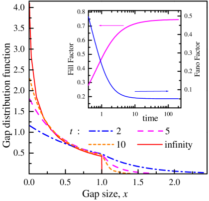
Figure 1: (Color online) Evolution with time of the averaged (over realizations) gap distribution function in the standard random parking problem; the inset show time variations of both the fill factor (Eq. 21) and the Fano factor (Eq. 52).

After reaching the jamming limit ($t\rightarrow\infty$), the gap distribution function becomes

$$G_{\infty}(x)=G(x,t)|_{t\rightarrow\infty}=\hskip 88.2037pt$$

$$=2\int_{0}^{\infty}dvv\exp\left[-xv-2\beta(v)\right]~{}.\hskip 28.45274ptx<1~{}.$$ (19)

Note a logarithmic divergence of (19) at small gap values

$$G_{\infty}(x\rightarrow 0)=2e^{-2\gamma}\ln\left(\frac{1}{x}\right),$$ (20)

where $\gamma=0.5772...$ is Euler’s constant. The average density of cars (and of gaps between them) at the time $t$ is given by

$$\rho(t)=\int_{0}^{t}dt^{\prime}e^{-2\beta(t^{\prime})}~{}.$$ (21)

It can also be written in terms of a rapidly converging integral, convenient for numerical evaluation

$$\rho(t)=-te^{-2\beta(t)}+2\int_{0}^{t}dt^{\prime}e^{-2\beta(t^{\prime})}e^{-t^{\prime}}~{}.$$ (22)

The growth of $\rho(t)$ saturates at the so-called jamming limit, when all gaps do not exceed the unit car size. The jamming state fill factor,

$$\rho_{\infty}=\int_{0}^{\infty}dt^{\prime}e^{-2\beta(t^{\prime})}=0.7475987...~{},$$ (23)

is known as the Renyi number.

Next, we use $G(x,t)$ to calculate the uncorrelated Fano factor, Eq. (7). In terms of the average gap size $\langle x\rangle$ the average density of cars $\rho(t)=(1+\langle x\rangle)^{-1}$ and

$$F_{unc}(t)=\rho(t)^{2}\langle x^{2}\rangle-[1-\rho(t)]^{2}~{}.$$ (24)

Integrating over the gap distribution in Eq. (24) and using Eq. (22) gives

$$F_{unc}(t)=2\rho(t)[1-\rho(t)]-1+\hskip 42.67912pt$$

$$2(1+t)\frac{\rho(t)}{t}e^{-2\beta(t)}+4\rho(t)I_{\beta}(t)~{},$$ (25)

where

$$I_{\beta}(t)=\int_{0}^{t}due^{-2\beta(u)}\left[\frac{1-(1+u)\exp(-u)}{u^{2}}\right]~{}.$$ (26)

Numerical evaluation of the integrals in the jamming state at $t\rightarrow\infty$ gives $F_{unc}\equiv F_{unc}(\infty)=0.0439766...$, which is smaller than the exact value, Eq. (2). The difference is not that large (about 14%) but still important so long as the contributions to the Fano factor from the correlation terms in the right-hand side of Eq. (13) are not estimated. In the next section we consider the contribution of these terms and show that in the jamming limit the nearest-neighbor correlation corrections are dominant.

Results obtained in this section are strictly valid for parking on the infinite line. However, we are obviously interested in finite parking lot lengths, corresponding to SEB of finite initial energy. The gap distribution function $G_{L}(x,t)$ suitable for the formulation of sequential parking on a line of finite length $L$ is discussed in Appendix A. In the limit $L\rightarrow\infty$, due to the self-averaging property, the function $G_{L}(x,t)\rightarrow G(x,t)$. Numerical experiments show that the two functions are identical within 1% already for $L\approx 6$. Therefore, the results obtained with Eq. (14) can be readily used for finite initial energies.

III.2 Evaluation of correlation effects

In the random parking model, evaluation of the correlation contributions to the Fano factor (Eq. 13) requires the knowledge of the pair distribution functions for the nearest-neighbor gaps, the gaps separated by two cars, three cars and so on. These are many-particle distribution functions and their evaluation is not an easy task.

To calculate the first correlation term, one needs the nearest-neighbor gap distribution function $G_{\infty}(x,x^{\prime})$. Fortunately, this function is known Rinto . It can be obtained as the long-time limit of the time-dependent function $G(x,x^{\prime},t)$ for which the kinetic equation is of the form

$$\frac{\partial G(x,x^{\prime},t)}{\partial t}=-[k(x)+k(x^{\prime})]G(x,x^{\prime},t)\hskip 28.45274pt$$

$$+\int_{x+1}^{\infty}dyG(y,x^{\prime},t)+\int_{x^{\prime}+1}^{\infty}dy^{\prime}G(x,y^{\prime},t)\hskip 28.45274pt$$ (27)

$$+~{}G(x+x^{\prime}+1,t)~{}.\hskip 71.13188pt$$

The source of correlation in Eq. (III.2) is seen to be contained in the last term on the right-hand side, which describes the appearance of two gaps $x$ and $x^{\prime}$ upon parking of a car in a gap of initial length $x+x^{\prime}+1$. We use the solution of Eq. (III.2) obtained in Rinto to write down the gap pair distribution function in the final state,

$$G_{\infty}(x,x^{\prime})=\lim|_{t\rightarrow\infty}G(x,x^{\prime},t)~{},$$ (28)

which is the nearest-neighbor distribution function in the jamming limit,

$$G_{\infty}(x,x^{\prime})=\int_{0}^{\infty}dt~{}t^{2}e^{-2\beta(t)}e^{-(x+x^{\prime})t}$$ (29)

$$+\frac{1}{2}\int_{0}^{\infty}dt_{1}e^{-\beta(t_{1})}e^{-xt_{1}}\int_{0}^{t_{1}}dt_{2}e^{-\beta(t_{2})}e^{-x^{\prime}t_{2}}J(t_{2})$$

$$+\frac{1}{2}\int_{0}^{\infty}dt_{1}e^{-\beta(t_{1})}e^{-x^{\prime}t_{1}}\int_{0}^{t_{1}}dt_{2}e^{-\beta(t_{2})}e^{-xt_{2}}J(t_{2})~{},$$

where

$$J(t)=1-e^{-2t}+2te^{-t}~{}.$$ (30)

Similarly to $G_{\infty}(x)$ in Eq. (19), the distribution function $G_{\infty}(x,x^{\prime})$ in Eq. (29) gives the number of pairs per unit length – but not the pair probability – and it must be properly normalized. By the definition of $G_{\infty}(x,x^{\prime})$, the integration over $x$ and $x^{\prime}$ gives

$$G_{\infty}(x)=\int_{0}^{\infty}dx^{\prime}G_{\infty}(x,x^{\prime}),\hskip 62.59596pt$$

$$\rho_{\infty}=\int_{0}^{\infty}dx\int_{0}^{\infty}dx^{\prime}G_{\infty}(x,x^{\prime})~{}.\hskip 59.75095pt$$ (31)

Hence, the normalizing factor is $(\rho_{\infty})^{-1}$.

The average two-gap product calculated with the distribution function $G_{\infty}(x,x^{\prime})$ can be written in the form

$$\int_{0}^{\infty}dx\int_{0}^{\infty}dx^{\prime}xx^{\prime}G_{\infty}(x,x^{\prime})=K_{1}+K_{2}+K_{3}~{},$$ (32)

where

$$K_{1}=\int_{0}^{\infty}dt~{}t^{2}e^{-2\beta(t)}I(t)^{2}~{},$$ (33)

$$K_{2}=\frac{1}{2}\left(\int_{0}^{\infty}dt_{1}e^{-\beta(t_{1})}I(t_{1})\right)^{2}~{}.$$ (34)

and

$$K_{3}=\int_{0}^{\infty}dt_{1}e^{-\beta(t_{1})}I(t_{1})\times\hskip 56.9055pt$$

$$\int_{0}^{t_{1}}dt_{2}e^{-\beta(t_{2})}I(t_{2})e^{-t_{2}}(2t_{2}-e^{-t_{2}}).$$ (35)

Here

$$I(t)=\int_{0}^{1}dx~{}x~{}e^{-tx}\equiv-\frac{d}{dt}\left(\frac{1-e^{-t}}{t}\right).$$ (36)

Note that both $K_{1}$ and $K_{2}$ are positive quantities. Numerical evaluations of the integrals gives:

$$K_{1}= 0.027982,$$

$$K_{2}= 0.072887,$$ (37)

$$K_{3}= -0.010512,$$

whence we find that the additional contribution to $F$ due to nearest-neighbor pair correlation is given by

$$\delta F_{nnp}=2\left[\rho_{\infty}(K_{1}+K_{2}+K_{3})-(1-\rho_{\infty})^{2}\right]$$

$$=0.007685~{}.$$ (38)

We see that the corrected value of the Fano factor including nearest-neighbor correlations only, $F_{nnp}=F_{unc}+\delta F_{nnp}=0.05208$, is above the exact value by only 0.001. One can anticipate that in a large parking lot gaps separated by two or more cars should be only slightly correlated. Indeed, due to the random nature of parking, only two nearest-neighbor gaps can be created in a single branching event, while gaps separated by two cars are created in two random events, which suggests that their sizes are not correlated. If that were the case for RPP, then the expansion (13) could be restricted to the nearest-neighbor correlation correction only, so that the approximation $F=F_{nnp}$ would be exact.

Temporal variation of the Fano factor including nearest-neighbor correlations only can be found similarly — with the help of $G(x,x^{\prime},t)$ — but the calculations become rather tedious. As an example, the values of $\delta F_{nnp}(t)$ for $t=8$ and $t=100$ are, respectively, $\delta F_{nnp}(8)=0.0052649004$ and $\delta F_{nnp}(100)=0.0074316483$. The calculated results are presented and discussed below, see Fig. 4.

In fact, all additional terms due to correlations in the positions of the 2nd, 3rd, …, neighbors are small but still non-vanishing, since every division of the parking length imposes restrictions on the further gap distribution. The next correction $\delta F_{2}$ due to the 2nd neighbors only is given by an equation similar to Eqs. (32, III.2), viz.

$$\delta F_{2}=2\rho_{\infty}\int_{0}^{1}\int_{0}^{1}dxdx^{\prime}xx^{\prime}G_{2}(x,x^{\prime})$$

$$\hskip 56.9055pt-2(1-\rho_{\infty})^{2}~{}.$$ (39)

Equation (III.2) is exact but the pair distribution function $G_{2}(x,x^{\prime})$ is exceedingly difficult to calculate because one needs to average an exact three-particle distribution function over the third particle position. Similar calculation for more distant pairs would require exact multi-particle joint distribution functions and averaging over all intermediate particle positions.

One can still make some progress by taking the factorization Ansatz for the multi-particle distributions, expressing them in terms of nearest-neighbor pair distributions. For the 2nd neighbor pair distribution function, this results in the following approximation

$$G_{2}(x,x^{\prime})=\int_{0}^{1}G_{\infty}(x,x^{\prime\prime})\frac{G_{\infty}(x^{\prime\prime},x^{\prime})}{G_{\infty}(x^{\prime\prime})}dx^{\prime\prime}~{},$$ (40)

where $G_{\infty}(x^{\prime\prime})^{-1}G_{\infty}(x^{\prime\prime},x^{\prime})\equiv G_{c}(x^{\prime\prime},x^{\prime})$ is the conditional probability of finding the second gap equal to $x^{\prime}$ for the case when the intermediate gap equals $x^{\prime\prime}$.

With the help of Eqs. (40, 31), it is convenient to rewrite Eq. (III.2) in the form

$$\delta F_{2}=2(1-\rho_{\infty})\int_{0}^{1}\int_{0}^{1}dxdx^{\prime}x^{\prime}G_{\infty}(x,x^{\prime})[r(x)-1],$$ (41)

where $r(x)$ is defined in terms of the ratio of the distributions

$$r(x)=\rho_{\infty}\frac{\int_{0}^{1}dx^{\prime}x^{\prime}G_{c}(x,x^{\prime})}{\int_{0}^{1}dx^{\prime}x^{\prime}G_{\infty}(x^{\prime})}~{}.$$ (42)

Function $r(x)$ reflects the conditional probability averaged with weight $x^{\prime}$ and it approaches unity when correlations are negligible (for $r=1$ all correlation corrections vanish).

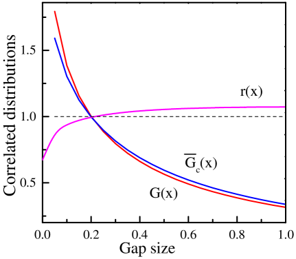
Figure 2: (Color online) Distribution ratio $r(x)$ and the conditional probability functions calculated under the factorization Ansatz (40).

With the factorization Ansatz, the correlation corrections for more distant pairs can be similarly expressed through integrals of $r(x)$ over conditional probabilities. Let us see how far we can get with this Ansatz.

The 2nd neighbor pair correlations described by Eqs. (40, 41, 42) are illustrated in Fig. 2, which shows the function $r(x)$ and also compares the functions $G_{\infty}(x)$ and

$$\overline{G}_{c}(x)=\rho_{\infty}\frac{\int_{0}^{1}dx^{\prime}x^{\prime}G_{\infty}(x,x^{\prime})}{\int_{0}^{1}dx^{\prime}x^{\prime}G_{\infty}(x^{\prime})}~{}.$$ (43)

needed for direct calculation of the first term in the right-hand side of Eq. (41). We see that both $G_{\infty}(x)$ and $\overline{G}_{c}(x)$ have a logarithmic singularity at $x\rightarrow 0$. Ratio $r(x)$ is on average close to unity and deviates from unity most noticeably at small $x$ where it approaches the value 0.504. Numerical calculations give for $\delta F_{2}=0.0011$ indicating that the Ansatz series converges. However, it does not converge to the exact value of $F$. Indeed, the positive sign of $\delta F_{2}$ excludes the possibility of reaching the exact value based on an accurate inclusion of only nearest-neighbor pair correlations. Evidently, rare multi-particle correlated configurations become important at this level of accuracy. The nature of these configurations is discussed in the next Section.

IV Discussion

Analytical expressions for the Fano factor in the jamming state of the RPP model have been obtained by several authors McKen ; Coffman ; Bonn . Since these authors used different techniques (a lattice model was used in McKen , a recursive approach was used in Coffman , and a kinetic approach was used in Bonn , whereby $F$ was obtained as a zero-wave-vector component of the structure factor), their final results were written in widely different forms, so much so that the equivalence of these results could be open to question. As shown in Appendix B, the results of McKen ; Coffman ; Bonn are indeed equivalent and can be cast in the following rather compact form:

$$F=2\rho_{\infty}-1-\frac{2}{\rho_{\infty}}\int_{0}^{\infty}\tilde{\rho}^{2}(t)e^{2\beta(t)}A(t)dt~{},$$ (44)

where $\tilde{\rho}(t)=\rho_{\infty}-\rho(t)$ and

$$A(t)=e^{-t}\left(\frac{e^{-t}+t-1}{t^{2}}\right).$$ (45)

Equation (44) yields the numerical value of the Fano factor, $F=0.0510387...$, that can be calculated with any required precision.

Numerical evaluation of the Fano factor with account of only the nearest-neighbor correlation somewhat differs (by 0.0021 or about 4%) from the exact value. This indicates that, contrary to the first intuition, distant gap correlations also give a contribution to $F$. This conclusion is supported by a more refined analysis of the correlations. The situation can be clarified by calculating the variance of $N$ recursively in parking lots of progressively increasing length. The procedure is described in Rusb ; ASSL and here we present (Fig. 3) only the results of calculations of the Fano factor as a function of the parking lot length $L$ (avoiding spurious edge effects, as described in Appendix A). One can clearly see very large variations of the Fano factor for short parking lot lengths, in the range of up to 5 cars. Such small gaps appear at an intermediate stage of the parking. These special correlations are completely smeared out only at $L>5$.

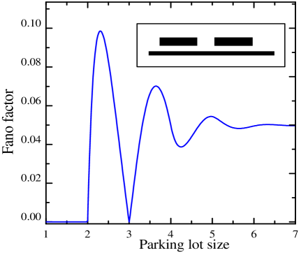
Figure 3: (Color online) The Fano factor for the random parking model calculated as a function of the parking lot length for small lots. Inset illustrates parking on a lot of length $L=3$. Even though the spacing between cars is chosen randomly, there are no fluctuations of the number of cars.

Consider a special case of random parking on a lot whose length is triple the size of a single car, as shown in the inset of Fig. 3. One can readily see that two cars will always park in this lot, with no fluctuation of this number (the unique case of three tightly parked cars with no gaps has zero probability). Clearly, the intermediate states of this type were not included in the preceding consideration and their contribution should reduce the resulting value of $F$ bringing it to the exact value.

Note that in the jamming state (where the fill factor is close to 3/4) three cars occupy an average length of $L\approx 4$. The typical space left for 2 cars equals 3 and the above configuration appears quite common. However, due to the nature of random parking, these configurations have different pre-histories and most of them result not from divisions of $L\approx 3$ lots. The overall contribution to $F$ of two-car lots remains positive. The negative contribution results mainly from the those configurations that have $L\approx 3$ lots in their history. In terms of sequential energy branching these configurations correspond to an intermediate state comprising a particle of energy $\approx 3E_{th}$. If such a particle is created in the course of SEB, the next energy branching will produce exactly 2 particles with no fluctuation, irrespectively of the fluctuating kinetic energies of these particles. Inclusion of this effect is the main residual correction contained in the distant pair correlation terms. For large initial energies, the overall contribution of these rare configurations at the jamming state should be $\delta F_{3}\approx-0.0021$.

It would be extremely interesting to realize a situation when configurations comprising a particle of energy $\approx 3E_{th}$ are not rare. For such configurations, the final state will be dominated by 2-particle contributions. Correlations of this type will suppress the fluctuations of the final number of particles in all cases when one of the secondaries produced at an intermediate stage regularly has a small energy. One possibility would be to look for these effects in the dependence of noise in semiconductor X-ray detectors on the frequency $\nu$ of incident X-ray flux of constant intensity. For $h\nu$ producing an initial electron of energy near $3E_{th}$ one can expect suppression of the noise component associated with the branching of energy of the photoabsorbed quanta.

There is also a tantalizing possibility to employ these correlations in practical $\gamma$-detectors, where the energy is, of course, much larger than $3E_{th}$. This possibility relies on the established fact that in semiconductors the dominant energy loss mechanism at high electron energies is plasmon emission rather than impact ionization Bichsel ; Gao . Plasmon emission can establish the dominant intermediate configuration — immediately preceding the final stage of SEB via impact ionization — that is populated with particles of energy close to the plasmon energy, which is $\approx 16$ eV in all common semiconductors. In the RPP language, the long parking lot, corresponding to the initial energy, would be divided at the intermediate stage into small 16 eV lots, where — as we have seen — the small-lot correlations can be very important.

As was noted in Sect. II, the kinetic approach allows to calculate both the filling factor and the Fano factor at any intermediate state — by using time-dependent distribution functions. Figure 4 compares the computed values of $F$ for the shot-glass model, where $F_{unc}(t)$ is given by Eq. (25), with exact results (Eq. 52) for the RPP model, both as functions of the line filling. The figure also shows the results obtained including the nearest neighbor correlations. Allowance for these correlations gives a very close upper estimate for $F$ for all stages of the random parking.

Inclusion of the correlation corrections obviously requires a computational effort. We believe it should be quite manageable because the only important correlations are those preceding the final state. Nevertheless, the shot-glass model remains attractive for its simplicity — as a 0-th order approximation — even though its use requires assumptions about the single-particle distribution that go beyond the model itself. In this vein, however, there is another statistical model that is, perhaps, even more attractive.

This model corresponds to a car distribution along the parking lot in which the probabilities of all allowable states are the same (as if all cars parked randomly at the same moment). This distribution is statistically equivalent to the model of a one-dimensional hard-rod (1D HR) gas, i.e. it can be viewed as an equilibrium spatial distribution of hard rods of unit length along a segment of a large total length with a given rod density $\rho$. For the 1D HR gas model one can calculate all multi-particle distribution functions exactly Sals . It was found that the gaps in the 1D HR model are distributed in accordance with Poisson statistics and that $F$ can be exactly expressed in terms of the filling factor $\rho(t)$, viz. $F=(1-\rho)^{2}$, see Appendix 3. In the 1D HR model, there is no jamming limit and the filling factor can take any value up to $\rho=1$. The choice of $\rho$, therefore, requires an assumption that goes beyond the model itself. The 1D HR model gives a simple way to estimate $F$ — whenever the filling factor is known. In a practical application of this model, it is natural to take the filling factor equal to the branching yield, $\rho=Y$, and estimate the latter consistently with the average pair excitation energy $\epsilon$. The 1D HR model gives an upper bound estimate that is fairly crude compared to the uncorrelated (shot glass) model, where the exact variance $\langle\delta\epsilon^{2}\rangle$ is plugged in.

Both the shot glass and the 1D HR model require assumptions external to the model itself: the 1D HR model needs the filling factor $\rho$, while the shot glass model needs the variance $\langle\delta\epsilon^{2}\rangle$ (derived here from the exact single-particle distribution).

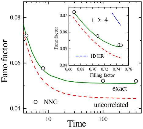
Figure 4: (Color online) Fano factor as a function of time for the RPP problem. The exact result is compared with the shot-glass model approximation (dashed line) with the exact variance $\langle\delta\epsilon^{2}\rangle$ plugged in. Open circles show the results obtained by allowing only the nearest neighbor correlations. The inset show the Fano factor as a function of the line filling factor in the region approaching the jamming state. It also shows the predictions of the 1D hard-rod gas model (dash-dotted line in the top right-hand corner).

At small values of $\rho$ all models give $F\approx 1-2\rho(t)$. For intermediate coverage, $\rho\leq 0.7$ and near the jamming state, the uncorrelated model gives a lower bound, while the 1D HR model an upper bound to the exact $F(t)$. We had already noted (at the end of Sect. 2) that in a real particle detector, the true jamming state is hardly achievable because the SEB slows down and is preempted by phonon emission and other energy loss mechanisms. Owing to the termination of the branching process at intermediate values of the filling time, the uncorrelated approximation becomes substantially less reliable.

A subtle conceptual problem with the uncorrelated approximation can be illustrated by a mock shot-glass model. Imagine that the man with the shot-glass watches what he is doing and compensates for an underfilled shot by following it with a shot with more than average filling, so that two successive glasses together scoop similar amount of water. Evidently, the fluctuations should be strongly reduced in this case, compared to predictions of Eq. (7). Moreover, it is precisely these types of correlations that are typical for the energy branching process. This is easiest seen in the parking model, where the division of any initial gap naturally pairs a small gap with a large neighbor gap. We shall refer to this effect as the “division correlations”. One could expect that the uncorrelated model — which ignores the division correlations — would give an overestimate of the Fano factor… but an inspection of Fig. 4 reveals that the opposite is true and the correlation correction to $F$ is positive. What is wrong with the above argument?

The answer lies in the fact that division correlations are not the only and not necessarily dominant correlation corrections. Consider the structure of the terms (33–35). Their physical meaning is revealed by the corresponding contributions to $G_{\infty}(x,x^{\prime})$ of Eq. (29). From the exponential dependences on $x$ and $x^{\prime}$ one can see that the term $K_{1}$ [originating from the 1st term in $G_{\infty}(x,x^{\prime})$] depends on the sum $x+x^{\prime}$ and thus is manifestly insensitive to division correlations. Term $K_{2}$ results from a combination of the 2nd and the 3rd terms in Eq. (29) with only unity retained from the $J$ of Eq. (30). This combination can be factorized and hence so can be $K_{2}=\langle x\rangle_{p}^{2}$, where the subscript $p$ indicates the “pair averaging” as in Eq. (34). The factorizable term does not represent division correlations either. The effect of division correlations resides apparently in the term $K_{3}$, which results from the remaining parts of $G_{\infty}(x,x^{\prime})$. It is indeed negative but its value is relatively small. As seen from Eq. (III.2), the term $K_{2}$ is dominant. Due to the nearest-neighbor correlations, the pair averaging gives a larger mean value than the single-particle averaging, $\langle x\rangle_{p}>\langle x\rangle$. This is undoubtedly related to the shape of the single-particle distribution function that peaks at low $x$.

V Conclusions

We have studied correlation effects in the fluctuation of the number of particles produced in semiconductor radiation detectors by impact ionization cascade that leads to sequential energy branching. Our analysis is based on an exactly soluble random parking model. First, we show that, in contrast to the so-called “final state” models, the accurate expression for Fano factor includes additional terms arising from the correlation between energies of the secondary particles created in the SEB process. Final state models, such as the “shot-glass” model, are widely used for estimation of the Fano factor in semiconductors, but they entirely neglect these correlations. We have considered the best (using an exact gap distribution function) predictions of the shot-glass model for the random parking model. We have found that the uncorrelated model — even with the exact distribution function — is not quite accurate and gives a lower bound to $F$.

Next, we considered the corrections arising from correlations between nearest-neighbor gaps, next nearest gaps and so on. Based on the exactly calculated pair distribution function, we found that nearest-neighbor pair correlations provide the dominant corrections and their inclusion brings $F$ very close to the exact value. The residual difference cannot be accounted for by a factorization Ansatz that expresses distant-neighbor pair distribution functions in terms of the nearest-neighbor distributions. Instead, one needs to take into account genuine multi-particle correlations.

The most important example of the correlated configuration that cannot be factorized into nearest-neighbor correlations is the intermediate state with the kinetic energy equal 3$E_{th}$ that will always branch into two particles, with no fluctuation of that number — irrespective of the fluctuating energies of these particles. We have discussed the possibility that this effect may produce an additional reduction of the Fano factor in semiconductors where the dominant energy-loss mechanism at high energies is plasmon emission.

More realistic models of energy branching in semiconductor gamma detectors comprise additional factors (such as non-random branching at the intermediate stages, energy-loss mechanisms and finite-width of the valence band) that make the correlation effects different from those calculated in the random parking model. However, their importance can be evaluated by the approach developed in this work.

A relatively crude upper estimate for the Fano factor can be obtained in the equilibrium statistical model of a one-dimensional hard-rod gas. The correlations in the 1D HR gas model are somewhat different from those of sequential energy branching and the model produces an upper bound to the exact result, provided the filling factor $\rho$ is known correctly. In this model, the Fano factor has a simple close-form expression in terms of $\rho$, but the latter is not limited by jamming and must be determined by considerations external to the model.

Appendix A Kinetics for a finite-size parking lot

Equation (14) for RPP and its extensions have been discussed in a number of papers (see Viot for the review) but only for the case of parking on an infinite line. The reason for this restriction has been that only on the infinite line the number of voids equals that of the cars and parking of a new car does not change this property. In a parking lot of finite length the number of voids exceeds the number of cars by unity, which seemingly makes the distribution function of voids not suitable for describing the current number of cars. However, one can consider an initial finite parking lot of length $L+1$ with one car fixed at the end. Then one can easily see that the numbers of cars and voids remain equal. The initial condition to the Eq. (14), corresponding to an empty lot, in this case takes the form

$$G_{L}(x,t)=\frac{1}{L+1}\delta(x-L)~{},\hskip 28.45274ptt=0~{}.$$ (46)

One can easily check that Eq. (46) satisfies the total length conservation condition,

$$\int_{0}^{\infty}dxG_{L}(x,t)+\int_{0}^{\infty}dxG_{L}(x,t)x=1~{}.$$ (47)

The time dependent filling factor $\rho(t)$ can either be calculated as the average number of cars per unit length,

$$\rho_{L}(t)=\int_{0}^{\infty}dxG_{L}(x,t)~{},$$ (48)

or, using Eq. (47), it can be expressed through the average size of the gaps.

In the limit $L\rightarrow\infty$, due to the self-averaging property, the function $G_{L}(x,t)\rightarrow G(x,t)$.

Appendix B Comparison of expressions for the Fano factor

An exact expression for the Fano factor in the RPP model was first derived by McKenzie McKen . In the form due to Coffman et al. Coffman , this result can be written as follows

$$F_{C}=\frac{4}{\rho_{\infty}}\int_{0}^{\infty}\tilde{\rho}(t)e^{-t}\left(\frac{1-e^{-t}}{t}\right)dt\hskip 28.45274pt$$

$$-\frac{4}{\rho_{\infty}}\int_{0}^{\infty}\tilde{\rho}^{2}(t)e^{2\beta(t)}e^{-t}A(t)dt-1~{},$$ (49)

where $A(t)$ is given by Eq. (45). The formula of Bonnier et al. Bonn in the same notations is given by

$$F_{B}=2\rho_{\infty}-1-\frac{4}{\rho_{\infty}}\int_{0}^{\infty}dte^{-2\beta(t)}\int_{0}^{t}dt^{\prime}e^{-2\beta(t^{\prime})}$$

$$\times\int_{0}^{t^{\prime}}dt^{\prime\prime}e^{2\beta(t^{\prime\prime})}A(t^{\prime\prime})~{}.\hskip 28.45274pt$$ (50)

To prove their identity, one can use in Eq.(B) the substitution (cf. Eq. 21)

$$\frac{d\tilde{\rho}(t)}{dt}=-e^{-2\beta(t)}$$ (51)

and then perform integrations by parts. This brings the integral of Eq. (B) into the form of the second integral in the right-hand side of Eq. (44). Similar simplification is achieved in the second term of the right-hand side of Eq. (49) by writing $\exp(-t)=\exp(-t)-1+1$ and then simplifying the term proportional to $2\exp[2\beta(t)][\exp(-t)-1]/t=d(\exp[2\beta(t)])/dt$ by integration by parts. The final result of the algebra is again of the form of Eq. (44). Therefore, both Eqs. (49) and (B) give identical results.

Evaluation of the Fano factor in the kinetic approach can be extended Bonn to include the temporal evolution of $F$. The exact $F(t)$ for the RPP model can be written in the form (simplified in the same way as Eq. B):

$$F_{B}(t)=2\rho(t)-1+2e^{-2\beta(t)}-\hskip 56.9055pt$$

$$-\frac{2}{\rho(t)}\int_{0}^{t}dt_{1}\tilde{\rho}(t,t_{1})^{2}e^{2\beta(t_{1})}A(t_{1})~{},$$ (52)

where $\tilde{\rho}(t,t_{1})=\rho(t)-\rho(t_{1})$. The temporal evolution of $F_{B}(t)$ is presented in the inset to Fig. 1.

Appendix C Fano factor for a one-dimensional gas of hard rods

In this ideal-gas model, the distances between neighboring particles are distributed according to the Poisson statistics Ziman , i.e.

$$G(x)dx=\overline{x}^{-1}e^{-x/\overline{x}}~{}dx~{}.$$ (53)

Moreover, in this model there is no correlation between the gaps separating different particles Sals and the pairwise gap distribution functions can be factored into products of single-particle functions (53). Therefore, only the first term survives in Eq. (13). The distribution (53) gives $\overline{x}^{2}-(\overline{x})^{2}=(\overline{x})^{2}$ and for a given line filling $\rho$ one has $\overline{x}=(1-\rho)/\rho$, so that in the notations of Eq. (13) $\langle\delta\epsilon^{2}\rangle=(1-\rho)^{2}/\rho^{2}$ and $\epsilon^{2}=(1+\overline{x})^{2}=\rho^{-2}$, resulting in

$$F_{hr}=(1-\rho)^{2}~{}.$$ (54)

This result was previously obtained by a much more complicated calculation. It involves finding the exact pair distribution function for the rods Sals and then calculating its Fourier transform (the structure factor), see e.g. Coll . The Fano factor is then given by the zero-momentum component of the structure factor. We were able to avoid these complexities by employing Eq. (13) and using the pair distribution function for gaps separating different particles rather than for particles themselves.

An alternative way of deriving the Fano factor in the hard-rod gas model is to use a general expression for the fluctuation of the number of particles in a given volume LL , valid for any thermodynamic system in equilibrium:

$$\langle(\Delta N)^{2}\rangle=-\frac{TN^{2}}{V^{2}}\left(\frac{\partial V}{\partial P}\right)_{T,N}~{}.$$ (55)

For the hard-rod gas, the equation of state is known exactly (see, e.g., Coll ), viz.

$$P(V-V_{0})=NT~{},$$ (56)

giving

$$\left(\frac{\partial V}{\partial P}\right)_{T,N}=-\frac{(V-V_{0})^{2}}{NT}~{}.$$ (57)

Substituting (57) into Eq. (55) and taking $\rho=V_{0}/V$, we again recover Eq. (54).

References

- (1) U. Fano, “Ionization Yield of Radiations. II, The fluctuations of the Number of Ions,” Phys. Rev. 72, 26 (1947).
- (2) W.E. Drummond and J.L. Moll, “Hot carriers in Si and Ge Detectors,” J. Appl. Phys. 42, 5556 (1971).
- (3) H. Bigler, “Fano Factor in Ge at 77 K,” Phys. Rev. 163, 238 (1967).
- (4) H. Spieler, Semiconductor Detector Systems, Oxford Univ. Press, 2005.
- (5) C. Klein, “Bandgap dependence and related features of radiation ionization energies in semiconductors,” J. Appl. Phys. 39, 2029 (1968).
- (6) R. Devanathan, L. R. Corrales, F. Gao, and W. J. Weber, “Signal variance in -ray detectors - a review,” Nucl. Instr. Meth. Phys. Res. A 565, 637 (2006).
- (7) D.V. Jordan, A. S. Reinolds, J.E. Jaffe, K.K. Anderson, L.R. Corralesa, and A. J. Peurrung, “Simple classical model for Fano statistics in radiation detectors,” Nucl. Instr. Meth. Phys. Res. A 385, 146 (2008).
- (8) W. van Roosbroeck, “Theory of the Yield and Fano Factor of Electron-Hole Pairs Generated in Semiconductors by High-Energy Particles,” Phys. Rev. A 139, 1702 (1965).
- (9) R.C. Alig, S. Bloom, and C.W. Struck, “Scattering by ionization and phonon emission in semiconductors,” Phys. Rev. B 22, 5565 (1980).
- (10) A.V. Subashiev and S. Luryi, “Fluctuations of the partial filling factors in competitive random sequential adsorption from binary mixtures,” Phys. Rev. E 76, 011128 (2007).
- (11) J.K. McKenzie, “Sequential Filling of a Line by Intervals Placed at Random and Its Application to Linear Adsorption,” J. Chem. Phys. 37, 723 (1993).
- (12) B. Bonnier, D. Boyer, and P. Viot, “Pair correlation in random sequential adsorbtion process,” J. Phys. A: Math. Gen. 27, 3671 (1994).
- (13) E. G. Coffman, Jr., L. Flatto, P. Jelenkovich, and B. Poonen, “Packing random intervals on-line,” Algorithmica 22, 448 (1998).
- (14) M. D. Rintoul, S. Torquato, and G. Tarjus, “Nearest-neighbor statistics in a one-dimensional sequential absorption,” Phys. Rev. E 53, 450 (1996).
- (15) The random parking problem considered here can be viewed as a one-dimensional example of a more general class of problems known as the irreversible random sequential absorption (RSA). For a thorough review of RSA models that include both 1D lattice models and various non-1D models, see e.g. J.W. Evans, “Random and cooperative sequential adsorption,” Rev. Mod. Phys. 65, 1281 (1993); more recent results are reviewed in Viot .
- (16) Similar models also arise in polymer chemical reactions. Thus, González et al. [J. J. González, P.C. Hemmer, and J. S. Høye, “Cooperative Effects in Random Sequential Polymer Reactions,” Chem. Phys. 3, 228 (1974)] have used an analogous model to study the kinetics of random sequential reactions (e.g. oxidation) for an infinite 1D polymer system when a reacted unit protects a certain number of its neighbors against the reaction.
- (17) B. Widom, “Random sequential addition of hard spheres to a volume,” J. Chem. Phys. 44, 3888 (1966).
- (18) E. M. Lifshitz and L. P. Pitaevsky, Physical Kinetics, (L. D. Landau and E. M. Lifshitz, Course of Theoretical Physics, Vol. 10), Oxford, U.K.: Pergamon, 1981.
- (19) The 1-d kinetic equation (14) can be obtained from the Boltzmann equation for a particle distribution function in the phase space by integrating it over the surface of constant energy, see V. N. Abakumov, V. I. Perel and I. N. Yassievich, Non-radiative Recombination in Semiconductors, North-Holland, Amsterdam (1991), Appendix 7.
- (20) H. Bichsel, “Straggling in thin silicon detectors,” Reviews of Mod. Phys. 60, 663 (1988).
- (21) F. Gao, L. W. Campbell, R. Devanathan, Y. L. Xie, Y. Zang, A. J. Peurrung, and W. J. Weber, “Gamma-ray interaction in Ge: A Monte-Carlo simulation,” Nucl. Instr. Meth. Phys. Res. B 255, 286 (2007).
- (22) J. Talbot, G. Tarjus, P. R. Van Tassel, and P. Viot, “From car parking to protein adsorption: an overview of sequential adsorption process,” Colloids and Surfaces. A 165 287 (2000).
- (23) Z. W. Salsburg, R. W. Zwanzig, and J. G. Kirkwood, “Molecular Distribution Functions in a One-Dimensional Fluid”, J. Chem. Phys. 21, 1098 (1953).
- (24) J. Ziman, Models of Disorder, Cambridge University, Cambridge, 1979, Chap. 6, p. 211.
- (25) B. Lin, D. Valley, M. Meron, B. Cui, H. My Ho, and S. A. Rice, “The Quasi-One-Dimensional Colloid Fluid Revisited”, J. Phys. Chem. B 113, 13742 (2009).
- (26) L. D. Landau and E. M. Lifshitz, Statistical Physics, 3rd Edition, Part 1, Oxford, U.K.: Pergamon, 1980, Sect. 112, p. 342.