Bohmian mechanics to high-order harmonic generation

Abstract

This paper introduces Bohmian mechanics (BM) into the intense laser-atom physics to study high-order harmonic generation. In BM, the trajectories of atomic electrons in intense laser field can be obtained with the Bohm-Newton equation. The power spectrum with the trajectory of an atomic electron is calculated, which is found to be irregular. Next, the power spectrum associated with an atom ensemble from BM is considered, where the power spectrum becomes regular and consistent with that from quantum mechanics. Finally, the reason of the generation of the irregular spectrum is discussed.

I Introduction

Atom interacting with the intense laser field (ILF) can absorb more than one photon and then emits photons at harmonics of the laser frequency, which is well known as high-order harmonic generation (HHG) Burnett1 ; ma ; Ferray . The harmonic spectrum has the following characteristics as a function of increasing frequency: a rapid decrease in harmonic intensity at first, followed by a plateau region with the harmonics having similar intensities; and then a rapid drop in harmonic strength beyond the plateau region. Recently, lots of theoretical works have studied this multiphoton phenomenon, including solving the time-dependent Schrödinger equation Burnett1 ; Zhou ; Qiao ; bian ; zzy ; zzy2 , the semiclassical trajectory methods, such as the three-step model Corkum and the Feynman’s path-integral approach in the strong field approximation Salieres ; Salieres2 ; eden , and even the classical trajectory method gb .

Bohmian mechanics (BM) Holland ; bohm ; Nikolic , or called quantum trajectory method rew , is another alternative formalism of quantum mechanics. In the early years, BM has been used to study some fundamental quantum phenomena such as the scattering by a square potential barrier joh ; cd and the diffraction through two slits cp . Recently, it has been applied to study and analyze many different processes and phenomena in physics and chemistry, such as atom-surface scattering ass3 ; ass , electron transport in mesoscopic systems xo , photodissociation of NOCl and NO₂ bkd , and the chemical reactions rew2 . Also, BM in terms of quantum trajectory has been considered to study chaos dd ; us ; mhp ; ce . Recently, it has been successfully applied to the intense laser-atom physics to study the dynamics of the above-threshold ionization (ATI) photoelectron by authors lcz .

In this paper, BM is introduced to the intense laser-atom physics to study HHG, which allows us to follow the time evolution of individual electron trajectory in atomic system first. We then calculate the power spectrum with the electron trajectory and find the corresponding spectrum is irregular. Next, we consider the power spectrum associated with an atom ensemble. In the atom ensemble, harmonic generation is determined by the Maxwell equation, where the electronic polarization of the atom ensemble plays a key role for the harmonic generation. We will show the electronic polarization of the atom ensemble gained from BM is equivalent to that obtained from quantum mechanics. On this condition, the power spectrum from BM is regular and consistent with that obtained from quantum mechanics. Finally, we will briefly discuss the reason why an individual electron trajectory generates the irregular spectrum.

This paper is organized as follow: We will briefly introduce quantum trajectory method first. Then we show the Hamiltonian for the hydrogen atom in ILF. In Sec. IV, we calculate the harmonic spectrum from a single electron trajectory, following by harmonic generation associated with an ensemble of atoms interacting with the ILF in Sec. V. Finally, we briefly discuss the reason of the generation of the irregular spectrum with an individual electron trajectory and then conclude.

II Quantum trajectory formalism of Bohmian mechanics

Quantum trajectory method comes from the following transformation of the time-dependent Schrödinger equation Holland ; bohm . Firstly a wave function can be written in the polar form $\psi(\mathbf{r},t)=R(\mathbf{r},t)\exp(iS(\mathbf{r},t)/\hbar)$. Secondly $\psi(\mathbf{r},t)$ is substituted into the time-dependent Schrödinger equation. Then the real part of the resulting equation is

$$\frac{\partial S}{\partial t}+\frac{\left(\nabla S\right)^{2}}{2m}+V+Q=0$$ (1)

and the imaginary part has the form

$$\frac{\partial\rho}{\partial t}+\nabla(\rho\mathbf{v})=0,$$ (2)

where $\rho(\mathbf{r},t)=R^{2}(\mathbf{r},t)$, $\mathbf{v}=\nabla S(\mathbf{r},t)/m$, and $Q(\mathbf{r},t)=-\frac{\hbar^{2}}{2m}\frac{\nabla^{2}R}{R}$. These two equations look like the classical Hamilton-Jacobi equation and the equation of continuity, respectively, except Eq. (1) has an extra term $Q$ which is usually called quantum potential in BM. Thus Eq. (1) is called the quantum Hamilton-Jacobi equation governed by an external potential $V$ and the quantum potential $Q$. The motion of particle is guided by the Bohm-Newton equation of motion, $md^{2}\mathbf{r}/dt^{2}=-\nabla(V+Q)$, or, equivalently, by

$$d\mathbf{r}/dt=\nabla S(\mathbf{r},t)/m.$$ (3)

In practice, we solve the time-dependent Schrödinger equation to obtain $\psi(\mathbf{r},t)$, and then $S(\mathbf{r},t)$. In this way, the quantum trajectory of the particle can be gained by integrating Eq. (3).

III Numerical solution of the time-dependent Schrödinger equation

The Schrödinger equation for Hydrogen atom in ILF can be written as (atomic units are used throughout)

$$i\frac{\partial\psi(\mathbf{r},t)}{\partial t}=[\widehat{H}_{0}(\mathbf{r})+\widehat{V}(\mathbf{r},t)]\psi(\mathbf{r},t).$$

Here $\widehat{H}_{0}(\mathbf{r})$ is the field-free Hydrogen atom Hamiltonian and $\widehat{V}(\mathbf{r},t)$ is the intense laser-atom interaction: $\widehat{H}_{0}(\mathbf{r})=-\frac{1}{2}\frac{d^{2}}{dr^{2}}+\frac{\widehat{L}^{2}}{2r^{2}}-\frac{1}{r},$ $\widehat{V}(\mathbf{r},t)=-\mathbf{r\cdot E}(t)=-zE(t),$ where the laser field is the linearly polarized field ($\mathbf{E}||\mathbf{z}$) and $E(t)$ is the laser field profile. Due to the linearly polarized laser field, magnetic quantum number $m$ of Hydrogen atom is a good quantum number, so that the problem of solving the time-dependent Schrödinger here can be simplified into a two-dimensional problem (see the inset in Fig. 1). In this work the solution of the time-dependent Schrödinger equation $\psi(\mathbf{r},t)$ is obtained by the grid method and the second-order split-operator method, which has been detailedly introduced by Tong et al xmt . The laser field profile is $E(t)=\left\{\begin{array}[]{ll}E_{0}\sin^{2}(\frac{\pi t}{20T})\sin(\omega_{0}t),&{0\leq t\leq 10T;}\\ E_{0}\sin(\omega_{0}t),&{t>10T,}\end{array}\right.$ where $T=2\pi/\omega_{0}$, and $E_{0}$ and $\omega_{0}$ are the electric field amplitude and angular frequency, respectively. We choose $E_{0}=0.0292$ a.u. (i.e., $I=3.0\times 10^{13}$W/cm²), and $\omega_{0}=0.0587$ a.u. (i.e., $\lambda=775$nm). The initial wave function $\psi(\mathbf{r},0)$ of the system is in the ground state of the field-free Hydrogen atom.

Figure 1: Power spectrum of the electron with the initial position $\mathbf{r}_{0}=(1.0$ a.u., $\pi/4)$. The inset shows the direction of the laser beam and the electron coordinate of atomic system.

IV Harmonic spectrum associated with a single electron trajectory

After obtaining the wavefunction $\psi(\mathbf{r},t)$, we can follow the time evolution of electron trajectory $\mathbf{r}(t)$ by integrating Eq. (3) with the electron initial position $\mathbf{r}_{0}$. According to BM Holland ; bohm ; Nikolic , the initial electron distribution is $|\psi(\mathbf{r},0)|^{2}$. In this work, $\psi(\mathbf{r},0)$ is the ground state of the field-free Hydrogen atom. Thus we can obtain an ensemble of electron trajectories with the corresponding electron initial positions. For an individual electron trajectory, the atomic dipole moment $\mu_{z}(t)$ along the laser polarization direction is $\mathbf{\hat{z}}\cdot\mathbf{r}(t)$. The corresponding power spectrum is gained by the Fourier transformation of the dipole moment gb ; kck :

$$P(\omega)=\left|\frac{1}{t_{f}-t_{i}}\int_{t_{i}}^{t_{f}}\mu_{z}(t)e^{-i\omega t}\right|^{2},$$ (4)

where $t_{i}=0$ and the propagation time $t_{f}$ is $35T$ in this work.

Explicitly, we take one atomic electron as an example with the initial position $\mathbf{r}_{0}=(1.0$ a.u., $\pi/4)$ in polar coordinates. The electron trajectory $\mathbf{r}(t)$ is calculated by integrating Eq. (3). The corresponding power spectrum is shown in Fig. 1 from Eq. (4). The spectrum has even harmonics, which is dominated by a Rayleigh scattering component at the laser frequency $\omega=\omega_{0}$. We have obtained lots of electron trajectories with different initial position $\mathbf{r}_{0}$ according to the initial electron distribution $|\psi(\mathbf{r},0)|^{2}$. The corresponding power spectra have the similar character described above. In the following, however, we will show the even harmonics of the power spectrum are coherently removed in an ensemble of atoms and the corresponding power spectrum is consistent with that obtained from quantum mechanics.

V Harmonic generation from an ensemble of atoms interacting with the intense laser field

The harmonic generation of an atom ensemble can be gained with the Maxwell equation al1 ; al2 ; al3 ; ya :

$$\nabla^{2}\mathscr{E}-\frac{1}{c^{2}}\frac{\partial^{2}\mathscr{E}}{\partial t^{2}}=\frac{4\pi}{c^{2}}\frac{\partial^{2}\mathscr{P}}{\partial t^{2}},$$

where $\mathscr{P}(\mathbf{r}^{\prime},t)$ is the electronic polarization of the atom ensemble at the point $\mathbf{r}^{\prime}$ and $\mathscr{E}(\mathbf{r}^{\prime},t)$ describes the electromagnetic field (involving the fundamental and the harmonic fields). Obviously, the electronic polarization $\mathscr{P}(\mathbf{r}^{\prime},t)$ plays a key role for the harmonic generation from the ensemble of atoms. We will show that the electronic polarization $\mathscr{P}(\mathbf{r}^{\prime},t)$ gained from BM is, approximately, equivalent to that obtained from quantum mechanics, i.e., both of their harmonic spectra from the atom ensemble are consistent.

We first assume the number of atoms is $N$ in a small volume $\Delta V$ near the point $\mathbf{r}^{\prime}$ in the atom ensemble ( $\Delta V\ll d^{3}$, where $d$ is the focal spot size of laser). The electronic polarization $\mathscr{P}(\mathbf{r}^{\prime})$ is defined as the atomic dipole moment per unit volume: $\mathscr{P}(\mathbf{r}^{\prime})=\sum\limits_{i}^{N}\mathbf{p}_{i}\mathbf{/}\Delta V$, where $\mathbf{p}_{i}$ is the atomic dipole moment of each atom in the small volume $\Delta V$. From the view point of quantum mechanics, the dipole moment of each atom is $p(t)=\left\langle\psi(\mathbf{r},t)|z|\psi(\mathbf{r},t)\right\rangle$ in the $\mathbf{\hat{z}}$ direction, where $\mathbf{r}$ is the electron coordinate of atomic system and $\psi(\mathbf{r},t)$ is the electron wavefunction. Thus the electronic polarization of the atom ensemble obtained from quantum mechanics is

$$\mathscr{P}(\mathbf{r}^{\prime},t)=Np(t)/\Delta V$$ (5)

in the $\mathbf{\hat{z}}$ direction.

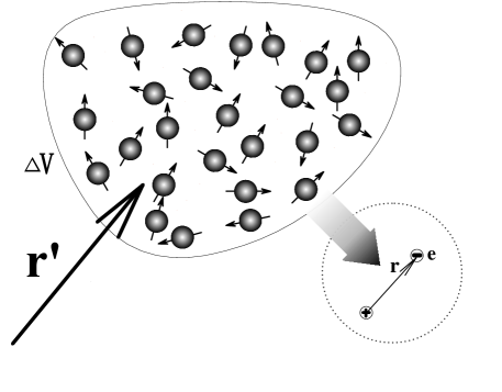
Figure 2: A small volume $\Delta V$ near the point $\mathbf{r}^{\prime}$ in the atom ensemble, which includes lots of atoms with the different dipole moments from the view of BM. The inset shows the electron coordinate of atomic system.

On the other hand, we calculate the electronic polarization of the atom ensemble from BM. According to BM Holland ; bohm ; Nikolic , the probability that an electron lies between $\mathbf{r}$ and $\mathbf{r}+\mathbf{dr}$ in the atomic system at the time $t$ is given by $|\psi(\mathbf{r},t)|^{2}\mathbf{dr}$, where the corresponding atomic dipole moment is $\mathbf{r}$ (in atomic units). Then in the small volume $\Delta V$ of the atom ensemble, the number of atoms with atomic dipole moment $\mathbf{r}$ is $(N|\psi(\mathbf{r},t)|^{2}\mathbf{dr})$. The sum of all kinds of atomic dipole moments in the volume $\Delta V$ is $\sum\limits_{j}N|\psi(\mathbf{r}_{j},t)|^{2}\mathbf{dr}_{j}\mathbf{r}_{j}$. Thus the electronic polarization $\mathscr{P}(\mathbf{r}^{\prime},t)$ at the point $\mathbf{r}^{\prime}$ in the atom ensemble is $\sum\limits_{j}N|\psi(\mathbf{r}_{j},t)|^{2}\mathbf{dr}_{j}\mathbf{r}_{j}/\Delta V$ (see Fig. 2). For an atom ensemble, we can replace the sum by an integral,

$$\sum\limits_{j}\frac{N|\psi(\mathbf{r}_{j},t)|^{2}\mathbf{dr}_{j}\mathbf{r}_{j}}{\Delta V}\rightarrow\frac{N}{\Delta V}\int|\psi(\mathbf{r},t)|^{2}\mathbf{r}d\mathbf{r}.$$ (6)

Further, because the laser field is the linearly polarized field ($\mathbf{E}||\mathbf{z}$), the time-dependent wavefunction $\psi(\mathbf{r},t)$ is symmetrical along $\mathbf{\hat{z}}$ axis. Thus in the $\mathbf{\hat{z}}$ direction,

$$\frac{N}{\Delta V}\int|\psi(\mathbf{r},t)|^{2}\mathbf{r}d\mathbf{r} =\frac{N}{\Delta V}\int|\psi(\mathbf{r},t)|^{2}r\cos\theta d\mathbf{r}$$

$$=\frac{N}{\Delta V}\int|\psi(\mathbf{r},t)|^{2}zd\mathbf{r},$$ (7)

where the last term equals Eq. (5). In this way, the electronic polarization $\mathscr{P}(\mathbf{r}^{\prime},t)$ gained from BM is, approximately, equivalent to that obtained from quantum mechanics, i.e., both of their harmonic spectra from the atom ensemble are the same. Figure 3 shows the harmonic spectrum from an ensemble of Hydrogen atoms interacting with ILF (laser confocal parameter $b=5.0$ mm, gas density $10^{17}$ atoms/cm³ described by a truncated Lorentzian in the $\mathbf{\hat{x}}$ direction with $L=0.5$ mm al1 ), which has a clear plateau region and cutoff at the $11$th order.

Figure 3: Harmonic spectrum associated with an ensemble of Hydrogen atoms at the laser field $I=3.0\times 10^{13}$W/cm² and $\lambda=775$nm.

VI Discussion

In BM, harmonic spectrum from a single electron trajectory has even harmonics (see Fig. 1), but they are removed in the spectrum associated with an ensemble of atoms (see Fig. 3). The reason is that an individual electron trajectory does not possess an inversion center gb , but the electron trajectories of the atom ensemble have such centre. Here we will numerically show that two electron trajectories are enough to get rid of the unphysical even harmonics if the initial positions $\mathbf{r}_{0}$ of the two electrons are centrally symmetric. Let’s take two electrons as an example with the initial positions $\mathbf{r}_{0}^{1}=(1.0$ a.u., $\pi/4)$ and $\mathbf{r}_{0}^{2}=(1.0$ a.u., $5\pi/4)$, respectively. The corresponding atomic dipole moment $\mu_{z}(t)$ along the laser polarization direction is $\mathbf{\hat{z}}\cdot[\mathbf{r}^{1}(t)+\mathbf{r}^{2}(t)]$ and the power spectrum gained from Eq. (4) is shown in Fig. 4 (solid curve), which has only odd-order harmonics. In addition, we calculate the HHG power spectrum in the length form from the time-dependent Schrödinger equation (dotted curve in Fig. 4) xmt . Note that these two curves can basically overlap if the value of the power spectrum from BM is multiplied by a factor of 0.4, i.e., both of them have the same relative intensity. This is an interesting result, but the reason why HHG power spectra from BM and the time-dependent Schrödinger equation have the same relative intensity should be studied in the future.

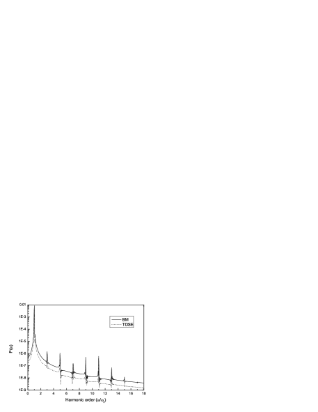
Figure 4: The solid curve corresponds to power spectrum of two Bohmian electrons with the centrally symmetric initial positions: $\mathbf{r}_{0}^{1}=(1.0$ a.u., $\pi/4)$ and $\mathbf{r}_{0}^{2}=(1.0$ a.u., $5\pi/4)$. The dot is the HHG power spectrum in the length form from the time-dependent Schrödinger equation (TDSE).

VII Summary

In summary, we introduce BM into the intense laser-atom physics to discuss HHG. It allows us to follow the time evolution of each electron trajectory in an atomic system. We find that the power spectrum from an individual electron trajectory has the even unphysical harmonics. But the even harmonics are coherently removed in the ensemble of atoms and the power spectrum is consistent with that obtained from quantum mechanics. The reason of the appearance of the even harmonics is an individual electron trajectory does not possess an inversion center, but the electron trajectories of the atom ensemble have such centre.

References

- (1) Burnett K, Reed V C and Knight P L 1993 J. Phys. B 26 561
- (2) McPherson A, Gibson G, Jara H, Johann U, McIntyre I A, Boyer K and Rhodes C K 1987 J. Opt. Soc. Am. B 4 595
- (3) Ferray M, L’Huillier A, Li X F, Lompr L A, Mainfray G and Manus C 1988 J. Phys. B 21 L31
- (4) Zhou X X and Lin C D 2000 Phys. Rev. A 61 053411
- (5) Qiao H X, Cai Q Y, Rao J G and Li B W 2002 Phys. Rev. A 65 063403
- (6) Bian X B, Qiao H X and Shi T Y 2007 Chin. Phys. 16 1822
- (7) Zhou Z Y and Yuan J M 2008 Chin. Phys. B 17 4523
- (8) Zhou Z Y and Yuan J M 2007 Chin. Phys. 15 2623
- (9) Corkum P B 1993 Phys. Rev. Lett. 71 1994
- (10) Salieres P, Carre B, Le Deroff L, Grasbon F, Paulus G G, Walther H, Kopold R, Becker W, Miloevi D B, Sanpera A and Lewenstein M 2001 Science 292 902
- (11) Salieres P, L’Huillier A, Antoine Ph and Lewenstein M 1999 Adv. At., Mol., Opt. Phys. 41 83
- (12) Eden J G 2004 Prog. Quantum Electron. 28 197
- (13) Bandarage G, Maquet A and Cooper J 1990 Phys. Rev. A 41 1744
- (14) Holland P R 1993 The Quantum Theory of Motion (England: Cambridge University Press)
- (15) Bohm D 1952 Phys. Rev. 85 166; Phys. Rev. 85 180
- (16) Nikolic H 2008 Am. J. Phys. 76 143
- (17) Wyatt R E 2005 Quantum Dynamics with Trajectories: Introduction to Quantum Hydrodynamic (New York: Springer); Lopreore C L and Wyatt R E 1999 Phys. Rev. Lett. 82 5190
- (18) Hirschfelder J O, Christoph A C and Palke W E 1975 J. Chem. Phys. 61 5435
- (19) Dewdney C and Hiley B J 1982 Found. Phys. 12 27
- (20) Philippidis C, Dewdney C and Hiley B 1979 Nuovo Cimento 52B 15; Philippidis C, Bohm D and Kaye R D 1982 Nuovo Cimento 71B 75
- (21) Sanz A S, Borondo F and Miret-Artés S 2004 Phys. Rev. B 69 115413; 2004 J. Chem. Phys. 120 8794; 2002 J. Phys.: Condens. Matter 14 6109; 2001 Europhys. Lett. 55 303; 2000 Phys. Rev. B 61 7743
- (22) Sanz A S and Miret-Artés S 2005 J. Chem. Phys. 122 014702
- (23) Oriols X 2007 Phys. Rev. Lett. 98 066803; Albareda G, Suñé J and Oriols X 2009 Phys. Rev. B 79 075315; Oriols X, Trois A and Blouin G 2004 Appl. Phys. Lett. 85 3596
- (24) Dey B K, Askar A and Rabitz H 1998 J. Chem. Phys. 109 8770
- (25) Wyatt R E 1999 J. Chem. Phys. 111 4406; 1999 Chemical Physics Letters 313 189; Pettey L R and Wyatt R E 2008 J. Phys. Chem. A 112 13335
- (26) Dürr D, Goldstein S and Zanghi N 1992 J. Stat. Phys. 68 259
- (27) Schwengelbeck U and Faisal F H M 1995 Phys. Lett. A 199 281; 1995 Phys. Lett. A 207 31
- (28) Partovi M H 2002 Phys. Rev. Lett. 89 144101
- (29) Efthymiopoulos C and Contopoulos G 2006 J. Phys. A 39 1819
- (30) Lai X Y, Cai Q Y and Zhan M S 2009 Eur. Phys. J. D 53 393
- (31) Tong X M and Chu S I 1997 Chem. Phys. 217 119
- (32) Kulander K C and Shore B W 1989 Phys. Rev. Lett. 62 524
- (33) L’Huillier A, Schafer K J and Kulander K C 1991 J. Phys. B 24 3315
- (34) L’Huillier A, Balcou P, Candel S, Schafer K J and Kulander K C 1992 Phys. Rev. A 46 2778
- (35) L’Huillier A, Li X F and Lompre L A 1990 J. Opt. Soc. Am. B 7 527
- (36) Akiyama Y, Midorikawa K, Matsunawa Y, Nagata Y, Obara M, Tashiro H and Toyoda K 1992 Phys. Rev. Lett. 69 2176