On Improving the Representation of a Region
Achieved by a Sensor Network

Abstract

This report considers the class of applications of sensor networks in which each sensor node makes measurements, such as temperature or humidity, at the precise location of the node. Such spot-sensing applications approximate the physical condition of the entire region of interest by the measurements made at only the points where the sensor nodes are located. Given a certain density of nodes in a region, a more spatially uniform distribution of the nodes leads to a better approximation of the physical condition of the region. This report considers the error in this approximation and seeks to improve the quality of representation of the physical condition of the points in the region in the data collected by the sensor network. We develop two essential metrics which together allow a rigorous quantitative assessment of the quality of representation achieved: the average representation error and the unevenness of representation error, the latter based on a well-accepted measure of inequality used in economics. We present the rationale behind the use of these metrics and derive relevant theoretical bounds on them in the common scenario of a planar region of arbitrary shape covered by a sensor network deployment. A simple new heuristic algorithm is presented for each node to determine if and when it should sense or sleep to conserve energy while also preserving the quality of representation. Simulation results show that it achieves a significant improvement in the quality of representation compared to other related distributed algorithms. Interestingly, our results also show that improved spatial uniformity has the welcome side-effect of a significant increase in the network lifetime.

I Introduction

Networks of inexpensive low-power sensor nodes may be deployed to sense, gather and process information in a region of interest for a variety of purposes including surveillance, target tracking, wildlife monitoring and pollution studies [1]. Based on the expected behavior of individual nodes, these applications of sensor networks may be broadly categorized into two types: area-sensing applications and spot-sensing applications. Examples of area-sensing applications include enemy surveillance, target tracking, intrusion detection and wildlife monitoring through audio/image/video recording; in these applications, sensor nodes make relevant observations within a local sensing area using vision, sound, seismic-acoustic energy, infrared energy, or magnetic field changes. On the other hand, in spot-sensing applications, each sensor node makes measurements of physical phenomena such as temperature, humidity and environmental pollution at precisely the spot where it is located, and there is no concept of a sensing area. The physical condition of each point in the region of interest is represented in the data collected from nearby active sensor nodes. The farther the nearest active nodes are from a point, the poorer is the representation of the physical condition at the point in the data collected by the sensor network. For example, if most of the active sensor nodes are clustered together in one corner of a region, the quality of representation of the region is likely to be poor. A more spatially uniform distribution, however, will lead to an improved quality of representation. In this report, we consider spot-sensing applications and introduce the problem of improving this quality of representation in the data collected by the sensor network.

The problem of improving the quality of representation is related but different from the coverage problems typically considered for area-sensing applications [2, 3, 4, 5, 6, 7, 8]. In most of these coverage problems, a region is considered $k$-covered if all points in it are within the sensing area of at least $k$ active nodes. Such a notion of coverage, while appropriate for area-sensing applications, is not relevant for spot-sensing applications where there is no concept of a sensing area. In spot-sensing applications, the quality of representation enjoyed by a point in the region depends on the desired spatial granularity with which the physical condition needs to be sampled and on some function of the distances to the nearest set of active sensor nodes around the point. This report introduces new metrics that help evaluate the quality of representation achieved by a sensor network deployed in a region.

Energy being a key constraint in most sensor networks, this work assumes that a sensor node can be programmed to make a choice at specific intervals of time on whether it should be in the sense mode (also referred in this report interchangeably as the active mode) or the sleep mode (in which its sensing module is turned off). An additional goal in spot-sensing applications becomes one of developing a distributed algorithm to determine sleep/sense times with the specific goals of (i) conserving energy, (ii) achieving the desired spatial granularity with which the physical condition in the region is sampled by achieving the appropriate spatial density of active nodes, and (iii) finally, achieving a high quality of representation of the region at all times by the network of active nodes.

The metrics for the quality of representation and the above goals of a distributed algorithm are also relevant in the context of sensor networks with transducer heterogeneity. It is becoming increasingly common in real world sensor network applications to integrate data from several different types of transducers [9, 10]. Microsensors, especially those using microelectromechanical systems (MEMS), permit the sensing of a variety of physical phenomena on a single sensor node [11]. Sensor nodes such as the Berkeley MICA Mote typically integrate several transducer types, such as for acceleration, temperature, light and sound, on a single board [12]. Each sensor node typically has dynamic control over which transducers are active. Since different physical phenomena generally require sensing at different spatial granularities, one can avoid unnecessary energy consumption by activating only a subset of transducers at each of the sensor nodes. This calls for distributed algorithms executed by all the sensor nodes to automate the process of determining which transducers should be activated on which nodes based on the desired density of each transducer type while also ensuring that all points in the region are well-represented by measurements made by each transducer type.

I-A Problem Statement

Consider $N$ sensor nodes distributed within a certain region of interest, denoted by $R$. Let $G^{\prime}=(V^{\prime},E^{\prime})$ denote the graph of these sensor nodes where each node $u\in V^{\prime}$ represents a sensor node and each edge $(u,v)\in E^{\prime}$ represents the fact that nodes $u$ and $v$ are neighbors and can communicate directly with each other. Let $d(u,v)$ denote the Euclidean distance between sensor nodes represented by vertices $u$ and $v$. The Euclidean distances between nodes are computable if the nodes are all fitted with low-power GPS receivers, or through location estimation techniques if only a subset of nodes are equipped with GPS receivers [13], or by estimating distances based on exchanging transmission and reception powers [14].

Let $z$ denote the desired spatial density, in number of active nodes per unit area, determined based on the spatial granularity with which the physical phenomenon of interest should be sensed. Let $G=(V,E)$ denote the subgraph of $G^{\prime}$ such that $v\in V$ iff vertex $v$ represents an active node (as opposed to one in sleep mode). In this report, we do not require that $G$ be a connected graph (because, in many applications, retrieval of data from sensor nodes may be accomplished through mobile gateways [15]). The problem now is one of determining $G$ in a distributed manner so that every point in the region is well-represented by the active sensor nodes.

There are two key aspects to this problem:

1. What are the metrics that one should use to measure the quality of representation achieved by $G$?

2. Given the metrics for quality of representation, what is a distributed algorithm that one should employ to determine $G$ (i.e., to determine which nodes should sense and which nodes should sleep) while achieving a high quality of representation?

I-B Contributions and Organization

We propose a new problem described in the previous subsection specifically for spot-sensing applications in sensor networks. We develop a pair of metrics that together allow a quantitative assessment of the quality of representation: the average representation error of the points in the region and the unevenness of representation error across the points in the region. Section II presents these metrics along with the rationale behind them. Based on the average representation error of the points in the region, Section II-A develops a metric normalized by the desired spatial density to allow for comparative evaluations of the quality of representation achieved by a network across different desired spatial densities. Section II-B borrows from the field of economics and uses the Gini index, a well-accepted measure of inequality, to develop a new metric for the unevenness of representation error among the points in the region. Section II-C discusses the need for both of these complementary metrics. Lower bounds on both metrics are derived in Section II-D. Upper bounds on these lower bounds for the common scenario of a continuous two-dimensional region covered by a sensor network are derived in Appendix A. Section III discusses work in sensor networks as well as in other fields which seek to solve similar or related underlying mathematical problems.

Section IV develops a generalized, distributed algorithm, called EvenRep($\cal{F}$, $L$), to achieve a better quality of representation for points in the region of interest. The algorithm, a simple heuristic, is parametrized by two quantities: $\cal{F}$, a target distance function which specifies the desired distance between an active node and its $k$-th nearest active neighbor and $L$, the maximum number of active neighbors that a node should consider in making its decision to sense or sleep. The algorithm seeks to achieve the target distance function for all active nodes. The target distance function, $\cal{F}$, can depend on whether the region of interest is 2-dimensional or 3-dimensional, the type of application, or any spatial constraints specific to the region. Section IV-A describes the pseudo-code of the algorithm and the rationale behind it. We find that the ideal target distance function is one based on the region of interest being tessellated by congruent hexagonal cells with an active sensor node at the center of each cell. We denote this target distance function by $H$ and Section IV-C describes EvenRep($H,L$), used in our simulation results.

Section V presents several simulation results on the performance of EvenRep($H,L$) and some other representative algorithms. The results show that the EvenRep($H,L$) algorithm achieves a significant improvement in the quality of representation in comparison to other algorithms. We show that achieving an improved quality of representation has a welcome side-effect of significantly improving the network lifetime. In fact, we show that EvenRep($H,L$) achieves almost a $50\%$ increase in the network lifetime in comparison to other related distributed algorithms. Section VI concludes the report.

II The Metrics

In this section, we develop metrics to quantify the quality of representation achieved in a sensor network deployment for spot-sensing applications. Past research that discusses related metrics has largely assumed a system model that is more appropriate for coverage problems in area-sensing applications [2, 3, 4, 5, 6, 7, 8]. In these problems, each sensor node has a pre-defined sensing range and the goal is to ensure that each point in the region of interest is $k$-covered, i.e., lies within the sensing area of at least $k$ active sensor nodes. As opposed to coverage at a point in an area-sensing application, the quality of representation of a point in a spot-sensing application is not easily captured in an either-or binary manner, an implication of the fact that there is no concept of a sensing area in spot-sensing applications. Even modified coverage problems for area-sensing applications, such as when a point is considered either covered or uncovered with a probability that is a function of the distance to the nearest sensor node [16], do end up imposing a binary either-or assessment that is not useful to assessing the quality of representation of the point. Also, metrics based on the distances between active nodes (e.g., [17]) used in solving different problems do not capture the quality of representation for spot-sensing applications, a quantity that is more about the points in the region of interest than the distances between neighboring active nodes.

The quality of representation of a point depends on the error in the representation of the point in the data collected by the sensor nodes. As mentioned in Section I, this error depends on some function of the distances between the point and the nearest active nodes. This function may be different for different physical conditions and is sometimes known (as discussed in [18]) but, most often, is unknown before network deployment. For clarity of presentation, we describe our work using the case in which the error in the representation of a point may be assumed to be directly proportional to the distance between the point and its nearest active sensor node (the error is zero if there is an active sensor node exactly at that point). However, the metrics of quality of representation that we develop can be readily adapted to other cases with different relationships between representation error at a point and the distances to the nearby active nodes. Further, the heuristic algorithm we present later in this report is also independent of this assumption. Also for clarity, we present this work assuming that the region covered by the sensor network is a $2$-dimensional plane. The metrics presented here and the algorithm can be readily adapted to the $3$-dimensional case.

Thus, the average of representation errors at all points in the region, normalized by the desired spatial granularity of active nodes for the physical condition being sampled, is one aspect of the quality of representation of the region. However, as we will show later in this section, a low average representation error alone does not tell the whole story and that an even spread of these values is also an essential aspect of the quality of representation. In the following, we formalize and develop a rigorous definition of two metrics: the average representation error based on the normalized average of the distances of the points to their respective nearest active nodes, and the unevenness of representation error based on the distribution of these distances.

II-A Average Representation Error

Let $d_{p}(v)$ denote the distance of node $v$ from point $p$. Let $n_{p}(G)$ denote the nearest node in $G$ (the set of active nodes) from point $p$. Let $\overline{d_{R}(G)}$ denote the average value of $d_{p}(n_{p}(G))$ over all points $p$ in region $R$. $\overline{d_{R}(G)}$ may also be thought of as the expected value of $d_{p}(n_{p}(G))$ for a random point $p$ in the region. Intuitively, given the same area of the region of interest and the same number of active sensor nodes, the smaller the value of $\overline{d_{R}(G)}$ the lower the representation error. However, as mentioned in Section I, the representation error should also depend on the desired spatial density of active nodes required for sampling of the physical phenomenon at the point (for example, particulate pollution may have to be sampled at a higher spatial granularity than temperature and so, the same average distances may not imply the same representation error). Different applications can tolerate different average distances between points and the nearest active nodes for the same quality of representation; therefore, without knowledge of the desired spatial density, $z$, the value of $\overline{d_{R}(G)}$ reveals little about the quality of representation achieved for an application. Therefore, an appropriate metric is one that uses the average distance, $\overline{d_{R}(G)}$, normalized by the average distance in the best-case scenario at the desired spatial density.

(a) One active node at the center of a unit square area.

(b) An active node placed at the center of each of the four quarters of a unit square area.

Figure 1: An example to illustrate the average representation error as a metric; $D(G,R)$ is the same in the two cases when the desired spatial density in (a) is 1 but in (b) is 4.

The best-case scenario occurs when the region of interest can be covered in a space-filling fashion by non-overlapping circular areas with an active sensor node at the center of each circular area. Note that such a scenario is not realistic and is used here only as a means to derive a normalization factor in the metric. Given a desired spatial density of $z$, the radius of these circular areas in the best-case scenario is given by $r=1/\sqrt{z\pi}$ (recall that $z$ denotes the desired number of active nodes per unit area, the size of each circular area is $\pi r^{2}$, and therefore, $z=1/\pi r^{2}$). The expected distance from points in the region to the nearest sensor node in this case is given by:

$$\int_{0}^{r}\frac{2\pi x}{\pi r^{2}}xdx=\frac{2r}{3}=\frac{2}{3\sqrt{z\pi}}$$

Thus, the normalized expected distance of points to their respective nearest nodes is given by:

$$\overline{d_{R}(G)}\left({\displaystyle\frac{3\sqrt{z\pi}}{2}}\right)$$

Dispensing with the constant, $3\sqrt{\pi}/2$, we define the average representation error, denoted by $D(G,R)$, as:

$$D(G,R)=\overline{d_{R}(G)}\,\sqrt{z}$$ (1)

Fig.  1 is illustrative of the average representation error as a metric. Consider a square region of interest of unit area. The average representation error in Fig.  1a when the desired spatial density is 1 is the same as the average representation error when the desired spatial density is 4.

II-B Unevenness of Representation Error

The field of economics has a long history of measuring inequality and a vast body of literature on the topic [19, 20]. For measuring the unevenness of representation error, we use a popular and well-accepted metric in economics, the Gini index, based on the relative mean difference between the quantities being compared (in our case, the quantities are distances of points to their respective nearest active sensor nodes). Consider $m$ quantities, $g_{1}\leq g_{2}\leq\dots\leq g_{m}$. The mean difference between these quantities is:

$$\Delta=\frac{1}{m^{2}}\sum_{i=1}^{m}\sum_{j=1}^{m}|g_{i}-g_{j}|$$

The relative mean difference is the mean difference divided by the mean, $\overline{g}$. The Gini index is defined as one-half of the relative mean difference, i.e.,

$${\rm Gini~{}index}=\frac{\Delta}{2\overline{g}}=\frac{1}{2\overline{g}m^{2}}\sum_{i=1}^{m}\sum_{j=1}^{m}|g_{i}-g_{j}|$$

Adapting the Gini index to the context of our problem poses one issue: the number of quantities we have is infinite because of the infinite number of points in any region of interest. Therefore, instead of using summations, we consider expected values in defining unevenness. Let $p$ and $q$ denote two arbitrary random points in the region of interest $R$. We define the unevenness of representation error, $U(G,R)$, of graph $G$ in the region $R$ as:

$$U(G,R)=\frac{E[|d_{p}(n_{p}(G))-d_{q}(n_{q}(G))|]}{2\overline{d_{R}(G)}}$$ (2)

where $p,q\in R$. The smaller the value of the above quantity, the better the spatial uniformity.

II-C One Metric or Two?

Figure 2: An example illustrating that improving $U(G,R)$ does not necessarily improve $D(G,R)$.

For both metrics, $D(G,R)$ and $U(G,R)$, a smaller value of the metric implies better quality of representation. A legitimate question at this point is whether minimizing one also minimizes the other, i.e., whether we need both of the above two metrics or if one of the metrics above can serve as the sole metric for measuring the quality of representation. We answer this using two simple examples: one in which $U(G,R)$ is minimized but $D(G,R)$ is not; another in which the $D(G,R)$ is minimized but $U(G,R)$ is not.

Does improving the evenness also improve the average? Fig.  2 considers two regions, each of unit square area but with different sensor node deployments for a desired spatial density of 1 (i.e., we wish to place exactly one sensor node in the region). In the first of the two regions, a sensor node is placed at the centroid of the area while in the other region, the node is placed at one of the corners of the square region. Note that both $D(G,R)$ and $U(G,R)$ are minimized in the former case for the desired spatial density of 1. Also note that $D(G,R)$ is maximized in the latter case. We now claim that the unevenness of representation is equal in the two cases and also the best achievable. The unevenness of representation error depends on the normalized distribution of the distances from the points in the region to the one active sensor node. Dividing the square region of interest into four quarters as shown in the region on the left-hand side in Fig.  2, we note that this distribution for points within each of the quarters is identical to each other. Since the overall distribution of these distances in the full square region of unit area is composed of the identical distributions within each of the quarters, the unevenness of representation in the region of unit square area in the left-hand side region is the same as that within each of the quarters. Now, the sensor node deployment shown in the region on the right-hand side of Fig.  2 can be thought of as an enlargement of one of the quarters in the region on the left-hand side, and therefore, achieving the same degree of evenness. This example shows that $U(G,R)$ can be the minimum possible when $D(G,R)$ is the minimum or the maximum possible. This shows that achieving the lowest possible unevenness of representation error does not necessarily achieve the best average representation error; in fact, sometimes it can even lead to the worst possible average representation error.

(a) A placement in which $U(G,R)$ is minimized but $D(G,R)$ is not.

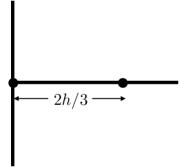
(b) A placement in which $D(G,R)$ is minimized but $U(G,R)$ is not.

Figure 3: An example illustrating that improving $D(G,R)$ does not necessarily improve $U(G,R)$.

Does improving the average also improve the evenness? Consider a toy example of a region composed of two one-dimensional regions arranged in the form of a sideways ‘T’ as shown in Fig.  3. Assume that the desired spatial density corresponds to placing two active sensor nodes in the region. Fig.  3a illustrates a placement in which $U(G,R)$ is minimized. Fig.  3b shows another placement of the two sensor nodes in which $D(G,R)$ is minimized but $U(G,R)$ is not minimized.

The two examples above show that improving the evenness does not necessarily improve the average representation error and that improving the average does not necessarily improve the evenness of representation error. Therefore, both metrics are essential to gaining insight into the quality of representation (though different metrics may rank differently in their importance to different applications).

II-D Lower Bounds on $D(G,R)$ and $U(G,R)$

For all of our subsequent analysis, it is insightful to have values of the lowest possible average representation error and the lowest possible unevenness of representation error. The following theorem proves these bounds.

Theorem II.1

The lower bound on $D(G,R)$ is $2/(3\sqrt{\pi})\approx 0.376$ and the lower bound on $U(G,R)$ is 0.2.

Proof:

The lower bounds of both $D(G,R)$ and $U(G,R)$ are achieved when the sensing nodes are perfectly evenly distributed such that the region of interest is completely covered by non-overlapping circular areas of radius $r$ with a sensing node at the center of each circle. Since each circle is identical to all others as far as the distances of all points to their nearest active nodes are concerned, $D(G,R)$ and $U(G,R)$ for each circular region are the same as $D(G,R)$ and $U(G,R)$ for the entire region.

The lower bound on $D(G,R)$ is the average distance between the center of a unit circle and the points within the circle. This is an easily-derived geometric result [21].

Focusing now on $U(G,R)$, note that the average distance between a point and the center of the circle is given by:

$$\overline{d}=\int_{0}^{r}\frac{2\pi x}{\pi r^{2}}xdx=\frac{2r}{3}$$ (3)

Consider two random points within such a circle at distances $x$ and $y$ from the center of the circle.

$$E[|x-y|]=\int_{0}^{r}\frac{2\pi x}{\pi r^{2}}\int_{0}^{r}\frac{2\pi y}{\pi r^{2}}|x-y|dydx=\frac{4r}{15}$$ (4)

Using Eqns.  (2) and (3):

$$U(G,R)=\left(\frac{1}{2}\right)\left(\frac{4r/15}{2r/3}\right)=\frac{1}{5}$$

∎

The bounds derived above are achieved in a scenario where the region of interest can be perfectly covered by non-overlapping circles. The simplest case would be a circular area with one sensor node placed at the center. While possible, this is an unlikely scenario for regions covered by a sensor network and therefore, in Appendix A, we consider regions of interest of arbitrary shape and prove upper bounds on the lower bounds of $D(G,R)$ and $U(G,R)$. Theorem A.1 in Appendix A shows that the lower bounds for regions of arbitrary shape are only slightly higher than those for the ideal case proved above.

III Related Work

The problem of designating the mode of a sensor node as either active or sleeping is related (though not identical) to the 2-color instance of some versions of the distributed graph coloring problem [22, 23], in which each node takes on one of two colors with the goal to minimize the number of neighbors of the same color as itself. While the algorithms in this body of work will generally improve the spatial uniformity of active nodes, they do not consider the distances between the nodes in their computations and therefore, are limited in their application to the problem under consideration. We show this later in Section V by simulating the Flip algorithm, an adaptation of the algorithm in [24], in which each node begins with randomly assigning itself one of two modes, and then, at random intervals of time, switches to the mode that best approximates the active node ratio in its neighborhood.

Spatially uniform distribution based on distances is more explicitly considered in another body of work related to the problem of facility location [25, 26]. The problem involves determination of the locations of facilities in an environment (such as emergency services in a city) given some constraints and an objective function. In the field of networking, related problems have been solved in the context of content distribution networks where one has to replicate resources in multiple locations (servers on a network) to boost performance by minimizing delay from users to the nearest resource or by achieving load balancing on the network [27, 28, 29, 30]. A variety of techniques, including graph-theoretic approaches, heuristic algorithms and dynamic programming, have been employed in these works to arrive at a solution. Ko and Rubenstein developed the first distributed algorithm for the placement of replicated resources, best described as a solution to the distributed graph coloring problem, by having each node continually change its color in a greedy manner to maximize its own distance to a node of the same color [31]. This work, which considers the distance between two nodes as that along the communication path and not as the geographical distance, cannot be directly applied to the problem considered in this report. A further reason this body of work does not directly apply here is that they only consider the relationships between nodes and not between the nodes and the points in the region of interest. Another set of works consider a set of points in the region of interest as the targets, where the goal is to cover and monitor each target point, as is discussed in [32]. This set of work also does not serve the purpose of achieving good quality of representation because, in our case, all points in the region are equally significant targets.

Points in the region of interest are most explicitly considered in the set of works that propose coverage algorithms for sensor networks based on assuming a sensing area for each node in area-sensing applications [2, 3, 4, 5, 6, 7, 8]. The goal is usually to ensure that each point in the region of interest is within the sensing area of at least $k$ active sensor nodes. Distributed algorithms to achieve $k$-coverage do not much improve the quality of representation although they do not specifically attempt it either. In Section V, we will compare the quality of sensor node representation and the lifetime of a representative member of this class of algorithms with the one proposed in this report.

IV The EvenRep($\cal{F}$, $L$) Algorithm

The design of a distributed algorithm for the problem stated in Section I-A requires that a node make an estimate of the quality of representation in its local area in comparison to the desired spatial density to reliably determine if it should sleep or go active. Note that even though the quality of representation is about the distances of points in the region to the nodes, only nodes and not the points can participate in this distributed algorithm and so, we have to use heuristics based on distances between nodes to achieve an improved quality of representation for the points. A node, therefore, needs to know the expected distances to the nearest active neighbors in a target distance function and compare these against the actual distances. Let $\cal{F}$ denote a target distance function which specifies a mapping between $k\geq 1$ and the target distance between an active node and its $k$-th nearest active neighbor. The origin of a target distance function, say $\cal{F}$, may be the expected distances between neighboring nodes in a given spatial distribution $\cal{S}$, but targeting $\cal{F}$ in the algorithm is not necessarily the same as targeting $\cal{S}$. For the same reason, $\cal{F}$ is not necessarily a mapping between $k$ and the expected distance between a node and its $k$-th nearest active neighbor in the spatial distribution $\cal{S}$.

Figure 4: The ideal sensor node layout which yields the target distance function, $H$.

The target distance function, $\cal{F}$, may depend on the environment and on the application. In our preliminary work, the EvenCover algorithm [33], we used a 2-dimensional plane with a non-ideal target distance function derived from a Poisson point process. In this work, we recognize that the Poisson distribution does not offer an ideal target distance function for improving the quality of representation. Given a 2-dimensional planar region of interest, it is known that the best representation is achieved when the region is tessellated in a space-filling manner by hexagonal cells with a sensor node placed at the centroid of each cell [34, 35]. This ideal layout is shown in Fig.  4 and we denote by $H$ the target distance function based on this layout. For a 3-dimensional region of interest, the ideal layout will be different and likely based on one of the space-filling tessellations of 3-dimensional space discussed in [36]. We propose a new algorithm which accepts any arbitrary target distance function, $\cal{F}$. Further, the algorithm presented here, EvenRep($\cal{F}$, $L$), allows a limit, $L$, on the number of active neighbors that a node will consider in its decision making process. The choice of $L$ in our implementation of the algorithm is discussed in Section IV-C.

IV-A Rationale and pseudo-code

 01: Initialization:  02: Turn on sense mode with probability $C_{z}$.  03: EvenRep($\cal{F}$, $L$) Algorithm (executes in a loop):  04: do:  05: if node is active:  06: $Q\leftarrow 1$  07: else:  08: $Q\leftarrow 0$  09: Wait for a random length of time between $0$ and $T$  10: $K\leftarrow\min$( number of active neighbors, $L$ )  11: Compile list of $K$ nearest active neighbors  12: for $1\leq k\leq K$:  13: $X_{k}\leftarrow$ distance to $k$-th nearest active neighbor  14: $Q\leftarrow Q+~{}T_{k}(\cal{F})$$/X_{k}$  15: if $(Q\geq z\pi X_{K}^{2})$:  16: if $(Q-z\pi X_{K}^{2}\geq 0.5)$:  17: Set node to sleep mode  18: else:  19: Set node to sleep mode with probability $(Q-z\pi X_{K}^{2})$  20: else:  21: if $(z\pi X_{K}^{2}-Q\geq 0.5)$:  22: Set node to active mode  23: else:  24: Set node to active mode with probability $(z\pi X_{K}^{2}-Q)$  25: while true

Figure 5: The EvenRep($\cal{F}$, $L$) algorithm executed at each node.

As before, let $N$ denote the total number of nodes in the region, $A$ the area of the region and $z$ the desired spatial density. Let $C$ denote the active node ratio, the fraction of nodes in the region of interest that are active. Note that $z$ is a property of the application and not of the sensor network used by the application, while $C$ describes the state of the sensor network. Let $C_{z}=zA/N$ denote the desired active node ratio. Denote by $T_{k}(\cal{F})$ the distance between the current node to its $k$-th nearest active node in the target distance function $\cal{F}$.

The pseudo-code for the algorithm executed at each node is shown in Fig.  5. Each node can compute a quantity $Q$ at the point where it is located based on a comparison between the actual distances to its nearest neighbors and their target values. Let $K$ denote the minimum of $L$ and the number of active neighbors within the node’s communication radius. Let $X_{k}$ denote the distance between the node and its $k$-th nearest active neighbor. Then, in the case in which the target distances are exactly achieved, $Q$ should equal the actual number of active neighbors within a radius of $X_{K}$. The expected number of nodes within radius $X_{K}$ at the desired active node ratio is $z\pi X_{K}^{2}$. A node should stay in its current mode or switch to a different mode depending on whether or not the action taken helps bring the $Q$ computed by it closer to $z\pi X_{K}^{2}$. For example, if the $Q$ computed is lower than that implied in the active node ratio, the node should go into the sense mode if not already in the sense mode.

Let $Q_{i}$ denote the $Q$ computed by node $i$. The algorithm computes $Q_{i}$ as:

$$Q_{i}=\delta_{i}+\sum_{k=1}^{K_{i}}\frac{T_{k}(\cal{F})}{X_{k,i}}$$ (5)

where $X_{k,i}$ is the distance from node $i$ to its $k$-th nearest neighbor, $K_{i}$ is the minimum of $L$ and the number of active neighbors of node $i$, and $\delta_{i}$ is given by:

$$\delta_{i} = \left\{\begin{array}[]{ll}1,&\mbox{if node}~{}i~{}\mbox{is in sense (active) mode},\\ 0,&\mbox{if node}~{}i~{}\mbox{is in sleep mode.}\end{array}\right.$$ (8)

Let $r_{i}$ denote the distance $X_{K,i}$. If $Q_{i}$ computed as above exceeds $z\pi r_{i}^{2}$ by $0.5$ or more and the node is in active mode, turning it to the sleep mode will bring the local active node ratio closer to that corresponding to the desired spatial density. Note that when a node goes from active to sleep mode, the number of active nodes in the local region of radius $r_{i}$ reduces by $1$ and, therefore, comparing the difference between $Q_{i}$ and $z\pi r_{i}^{2}$ against $0.5$ allows the node to best decide if it should sense or sleep so that $Q_{i}$ is as close to $z\pi r_{i}^{2}$ as possible after it makes the decision. Similarly, if $z\pi r_{i}^{2}$ exceeds $Q_{i}$ by $0.5$ or more and node $i$ is in sleep mode, turning it to the active mode will also bring the local active node ratio closer to that corresponding to the desired spatial density. If $Q_{i}$ exceeds $z\pi r_{i}^{2}$ by less than $0.5$, the algorithm sets the node to sleep mode with probability equal to $Q_{i}-z\pi r_{i}^{2}$ (this does not necessarily bring the local spatial density closer to the desired value but is an attempt to bring the overall active node ratio of the network closer to that corresponding to the desired spatial density). Similarly, if $z\pi r_{i}^{2}$ exceeds $Q_{i}$ by less than $0.5$, the node is set to active mode with probability $z\pi r_{i}^{2}-Q_{i}$.

IV-B Complexity analysis

We now examine the computational, communication and memory complexity of the EvenRep($\cal{F}$, $L$) algorithm separated from any topology control algorithm running at each node and entrusted with maintaining a list of active neighbors within the node’s communication radius. Note that the execution of line 11 has computational complexity $O(1)$ because each sensor node has to compile $K\leq L$ active neighbors where $L$ is a small constant. During the execution of lines 12-14, the node updates $Q$ based on the distances between itself and up to $K$ neighbors, each of which takes $O(1)$ time. Again, since $K\leq L$, a small constant, this too adds a complexity of only $O(1)$. The rest of the algorithm is also $O(1)$ and therefore, the computational complexity of the algorithm at each node is $O(1)$. The communication complexity of EvenRep($\cal{F}$, $L$) is also $O(1)$, assuming again that a separate and independent topology control algorithm maintains a list of active neighbors. The memory usage of the algorithm is in the order of $O(1)$.

Note that the topology control algorithm, running independently of EvenRep($\cal{F}$, $L$), may have its own communication complexity associated with each node having to broadcast its active state to its neighbors, receiving an acknowledgement for it from each of its active neighbors and also receiving such state from each of its active neighbors. This communication complexity depends on the topology control algorithm used (which can vary greatly depending on the algorithm [37, 38, 39]) and also on method used to estimate the distance to each active neighbor (such as whether it is based on assuming GPS devices in the sensor nodes [13] or on exchanging transmission and reception powers [14]).

IV-C EvenRep($H,L$)

In the following, we focus on $\cal{F}$ $=H$ as the target distance function and compute $T_{k}(H)$ for use in the EvenRep($H,L$) algorithm. In the perfect layout (shown in Fig.  4), upon which the target distance function $H$ is based, each active node has six equidistant active neighbors. Assuming an arbitrary distribution of sensor nodes in a region with a given node density $z$, the expected radius of a circular region that contains seven active nodes is $r=\sqrt{7/(\pi z)}$. To achieve a correspondence to a perfectly uniform distribution such as in Fig.  4, the heuristic EvenRep($H,L$) uses a target distance of $\sqrt{7/(\pi z)}$ from an active node to each of its six active neighbors.

Coincidentally and conveniently, for most topology control algorithms, the number of active neighbors is typically $6$ or smaller [37, 38, 39]. Therefore, we provide here the target distance function only for $k\leq 6$:

$$T_{k}(H)=\sqrt{\frac{7}{\pi z}},\ \mbox{if}~{}k\leq 6\\$$ (9)

The EvenRep($H,L$) algorithm analyzed in this report uses the above expression for the target distance function $H$, and with $L$ set equal to 3. This choice of $L$ is based on our finding that the fourth neighbor and beyond (i) have a diminishing influence on the quality of representation within the local region of the node, and (ii) are better and more effectively considered at other nodes for which they are one of the three closest neighbors.

V Simulation Results

Our simulation experiments use $1000$ sensor nodes located in a square region of unit area with a spatial distribution given by a Poisson point process (each point in the region is equally likely to have a node). In our implementation of EvenRep($H,3$), we choose $T$ as equal to 10 units of time (recall from line 9 of the pseudo-code in Fig.  5 that each node waits a random length of time between $0$ and $T$ between making the sense/sleep decisions). The desired spatial density, the corresponding active node ratio and the communication radius used in the experiments are described as we discuss each of the simulation experiments in the following subsections.

Each data point reported in the figures in this section represents an average of $200$ different simulation experiments (each using a different initial layout of the nodes). Based on the method of batch means to estimate confidence intervals, we have determined that the 95% confidence interval is within $\pm 1$% for each of the data points reported in the graphs.

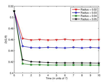
(a) Average representation error, $D(G,R)$, achieved by EvenRep($H,3$) plotted against time from $0$ to $10T$ for different values of the communication radius.

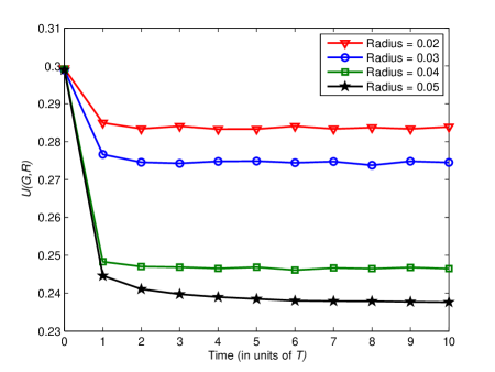
(b) Unevenness of representation error, $U(G,R)$, achieved by EvenRep($H,3$) plotted against time from $0$ to $10T$ for different values of the communication radius.

Figure 6: Plots showing the convergence of EvenRep($H,3$) as the algorithm executes and improves the quality of representation. In these experiments, the desired spatial density used corresponds to an active node ratio of $0.35$.

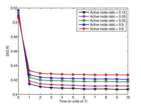
(a) Average representation error, $D(G,R)$, achieved by EvenRep($H,3$) plotted against time from $0$ to $10T$ for different values of the desired active node ratio.

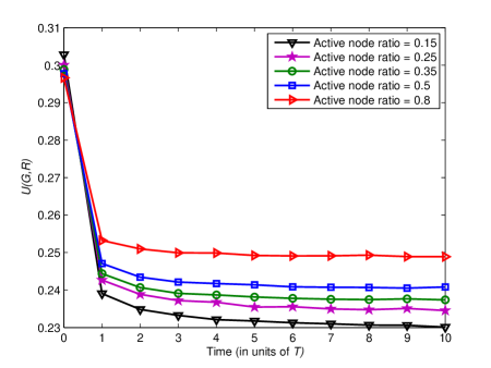
(b) Unevenness of representation error, $U(G,R)$, achieved by EvenRep($H,3$) plotted against time from $0$ to $10T$ for different values of the desired active node ratio.

Figure 7: Plots showing the convergence of EvenRep($H,3$) as the algorithm executes and improves the quality of representation. In these experiments, the communication radius used is 0.08.

Our algorithm begins with each node randomly setting itself to active mode with probability equal to $C_{z}$, the expected active node ratio when the desired spatial density is $z$. Thus, the spatial distribution of active nodes at the beginning of the simulation is given by a finite Poisson point process. To understand the reference point at which the simulation begins, we prove an additional set of results in Appendix B on the two metrics. Theorem B.1 in Appendix B proves that when the active nodes are located in the region with a spatial distribution given by a Poisson point process, the expected value of the average representation error, $D(G,R)$, is $0.5$ and the expected value of the unevenness of representation error, $U(G,R)$, is $1-1/\sqrt{2}\approx 0.293$. Due to the use of a finite Poisson point process for the initial layout of the nodes in the unit area in our simulation experiments, border effects cause the initial values of $D(G,R)$ and $U(G,R)$ to be slightly larger than $0.5$ and $1-1/\sqrt{2}$, respectively. Recall from Theorem II.1 that a lower bound on $D(G,R)$ is $2/(3\sqrt{\pi})\approx 0.376$ and a lower bound on $U(G,R)$ is $0.2$. Therefore, in our simulation experiments, one should expect that $D(G,R)$ reduces to something between $0.5$ and $0.376$ and that $U(G,R)$ reduces to something between $0.293$ and $0.2$ after a certain length of time since the beginning of algorithm execution.

V-A Convergence

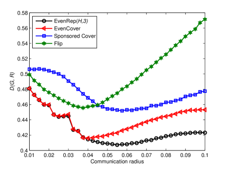
(a) Average representation error, $D(G,R)$, achieved after time $5T$ by different algorithms plotted against the communication radius.

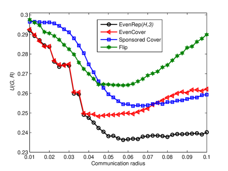
(b) Unevenness of representation error, $U(G,R)$, achieved after time $5T$ by different algorithms plotted against the communication radius.

Figure 8: Plots comparing the quality of representation achieved by different algorithms.

Fig.  6 shows the convergence of the EvenRep($H,3$) algorithm on the quality of representation metrics, $D(G,R)$ and $U(G,R)$, for different values of the communication radius while the desired spatial density corresponds to an active node ratio equal to $0.35$ (i.e., given $1000$ nodes in the unit area in our simulations, the desired spatial density, $z$, corresponds to $350$ active nodes). Almost all topology control algorithms achieve an average communication radius at each node corresponding to six or fewer neighbors [38, 39]. Therefore, the largest communication radius we use is $0.08$ units, which corresponds to approximately $6$ active neighbors within a node’s communication radius.

Fig.  6a plots the average representation error as the algorithm continues to execute for a length of time equal to $10T$. Fig.  6b shows the corresponding convergence of the EvenRep($H,3$) algorithm on the unevenness of representation error metric using the same set of parameters. Note that both the average and the unevenness of representation error reduce rapidly as early as $T$ (about $2$ iterations of the loop between lines 04–25 in Fig.  5 because the expected length of time between two iterations is $T/2$). It is not necessarily true that as the communication radius increases, the average representation error, $D(G,R)$, will reduce. This is because, when the communication radius is small, in order to achieve the desired active node density more nodes than necessary will determine that they should be active since they have limited information about the status of other nodes in the region. This reduces the average distance between active nodes, thus reducing $D(G,R)$, but does not necessarily improve $U(G,R)$. As one might expect, as the communication radius increases, each sensor node has more neighbors and is able to collect significantly more relevant information about the quality of representation in its neighborhood, thus reducing the unevenness of representation error.

In our second set of experiments on the convergence properties of EvenRep($H,3$), we keep the communication radius constant and vary the desired active node ratio from 0.15 to 0.8. We use a communication radius of 0.08 units corresponding to an average of about six active neighbors within the radius when the active node ratio is 0.35 (the density used in the previous set of experiments). The result is plotted in Fig.  7a and Fig.  7b for an interval of time up to $10T$. Once again, the algorithm appears to converge rapidly within time $T$, which corresponds to approximately $2$ executions of the algorithm for each sensor node. Note that the algorithm’s performance does not increase with the increase of the active node ratio. In this set of experiments, the algorithm achieves its best performance when the active node ratio is 0.15, the smallest ratio used in the experiments. This is expected because, when the active node ratio is high, the algorithm has fewer choices in determining the active node layout and becomes more confined to the original Poisson distribution of the nodes; on the other hand, when the active node ratio is low, the algorithm has more choices in determining which nodes should sense and which should sleep, leading to an improved quality of representation. A theoretical proof of the convergence of the algorithm remains an open problem.

It should be noted that, while fast convergence to low values of these metrics is desirable, convergence to one particular layout of the active nodes is not desirable. This is because the lifetime of a network suffers if nodes, once chosen to be active, remain active forever.

V-B Comparative analysis

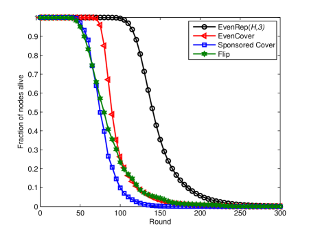
(a) The fraction of nodes alive as the execution of an algorithm proceeds.

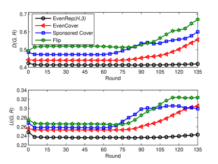
(b) The quality of representation as the execution of an algorithm proceeds.

Figure 9: Plots showing the network lifetime (the fraction of nodes alive is used as in indication of network lifetime) and the degradation in the quality of representation as nodes die. The communication radius used is $0.08$ units.

We report results for the following distributed algorithms:

• The EvenRep($H,3$) algorithm: The EvenRep($\cal{F}$, $L$) algorithm using a target distance function $\cal{F}$ $=H$ (based on a node placement in which the region is covered by non-overlapping hexagonal cells with each sensor node covering one cell) and $L=3$. The value of $T_{k}(H)$ used in the algorithm implementation is discussed in Section IV-C (see Eqn.  (9)).

• The EvenCover algorithm: This is our preliminary work [33] that employs a target distance function derived from a distribution of sensor nodes given by a Poisson point process.

• Sponsored Cover: For a representative coverage protocol that assumes an area-sensing application, we choose the well-cited coverage-preserving node-scheduling scheme based on sponsored coverage calculations [40]. In this protocol, a node decides to go into the sleep mode if its entire designated sensing area is also covered by its neighbors. To avoid situations in which each of two neighbors expects a certain spot to be covered by the other, the protocol implements a random time for which each node delays its decision.

• Flip: In this protocol, each node counts the fraction of its neighbors (including itself) that are active and sets itself into either the sleep mode or the active mode depending on whether or not this fraction is larger or smaller than the desired active node ratio. We use this algorithm as representative of coverage strategies based on distributed algorithms for graph coloring that do not use the distance between the nodes in their computations [23].

Figs.  8a and 8b plot the performance of these algorithms against the communication radius after the algorithms execute for a period of time $5T$. The Sponsored Cover algorithm takes the communication radius as the sole input while the other three also require the desired active node ratio as an input (chosen as $0.35$ in these figures). The figures show that EvenRep($H,3$) achieves the best quality of representation among the algorithms studied. Given that the target distance function $H$ is based on a more spatially uniform distribution of nodes than a Poisson point process (upon which the EvenCover algorithm is based), one expects the EvenRep($H,3$) algorithm to perform better than EvenCover (as is also observed in these results). The Sponsored Cover algorithm seeks full, but not necessarily even, coverage of points in the region. As a result, in parts of the region with a denser cluster of nodes, the Sponsored Cover algorithm will unnecessarily turn on larger numbers of nodes resulting in poorer spatial uniformity. The Flip algorithm, on the other hand, does not consider distances between nodes and therefore, is far from being able to achieve a good quality of representation.

V-C Network Lifetime

In this section, we compare the network lifetime of EvenRep($H,3$) with other algorithms. In our simulation experiments, we begin with each node allocated a certain amount of energy which is expended in the following two ways:

• On/off broadcast transmission, used to broadcast the node’s new status (on/off) to its neighbors.

• Reception, for receiving data and control information from neighbors.

The power consumption model is adapted from [40], with the assumption that each node is allocated 0.05J of energy and the data signal is a 2000-bit report message. The transmission energy consumption and the reception energy consumption is calculated as follows:

$$E_{T_{x}}(d) = E_{elec}\times k+\varepsilon_{friss\mbox{-}amp}\times k\times d^{2}$$ (10)

$$E_{R_{x}} = E_{elec}\times k$$ (11)

where $E_{T_{x}}(d)$ is the energy consumed in transmitting the signal to an area of radius $d$, $E_{elec}$ is the energy consumed for the radio electronics, $\varepsilon_{friss\mbox{-}amp}$ is for the power amplifier and $E_{R_{x}}$ is the energy consumed in receiving the signal. Radio parameters are set as $E_{elec}=50nJ/$bit and $\varepsilon_{friss\mbox{-}amp}=10pJ/$bit$/m^{2}$. The energy consumed in sensing is not considered in this set of simulations, exactly as in the model used in [40].

The EvenRep($\cal{F}$, $L$) algorithm does not use the concept of rounds while Sponsored Cover and Flip do. In order to present a fair comparison, therefore, we use a slightly modified version of our algorithm so that each node is scheduled to work in rounds. At the beginning of each round, each node randomly picks a start time, $t$, between $0$ and $T$, and makes its decision based on the information received so far. At time $t$ after the start of the round, it switches its state according to the decision made. If the node chooses to turn on, then it will broadcast its decision to its neighbors. Each of its neighbors will receive the decision and remember it for its own reference. If the node chooses to turn off, it will not make any broadcast attempts. A node is considered dead if it has consumed all the power allocated and alive, otherwise. Once a node is dead, it cannot be turned on again nor can it broadcast or receive signals.

A fair lifetime comparison can only be achieved when both the communication radius and the active node ratio are the same for each of the four listed algorithms. Recall that the Sponsored Cover algorithm does not require the active node ratio as an input. However, since the active node ratio achieved by the Sponsored Cover algorithm is a function of the communication radius employed, it strictly limits the choice of the desired active node ratio we can use in our comparisons. In these experiments, we use a communication radius of $0.08$ units for all four algorithms. Using this communication radius, we first note the active node ratio achieved by the Sponsored Cover algorithm and then use this ratio as the input active node ratio for the other three algorithms.

Fig.  9a reports the fraction of nodes alive as time progresses to indicate the network lifetime (for example, one may define network lifetime as the time until 50% of the nodes are dead). Figs.  9a and 9b demonstrate that the EvenRep($H,3$) algorithm significantly improves the lifetime of the network while also achieving a better quality of representation even as nodes die. Since the Sponsored Cover algorithm seeks area-sensing coverage of points in the region, some sensor nodes may have to constantly stay active while its neighbors are constantly in sleep mode. The goal of full coverage, therefore, contributes to a reduced lifetime while the goal of spatial uniformity, appropriate for spot-sensing applications, results in an improved lifetime. The combination of striving for spatial uniformity and the use of random chance to place nodes in specific modes (as in lines 19 and 24 in Fig.  5) leads to the difference between the lifetime achieved by EvenRep($H,3$) and that achieved by other algorithms. In addition to improved lifetime, Fig.  9b shows that the EvenRep($H,3$) algorithm better preserves the average and the evenness of representation error as nodes in the network die, in comparison to other algorithms. This indicates that EvenRep($H,3$) achieves a more graceful degradation of the sensor network as the battery power in the nodes are exhausted. The EvenCover algorithm, on the other hand, does not achieve as good a lifetime. As can be observed from Figs.  8a and 8b, the EvenCover algorithm performs as well as EvenRep($H,3$) when the communication radius is small (corresponding to 4 or fewer active neighbors). However, a communication radius corresponding to an average of 6 active neighbors is a more realistic scenario generated by topology control algorithms and EvenRep($H,3$) performs significantly better in this range of the communication radius.

VI Conclusion

Recent research literature has largely focused on area-sensing applications where the goal is to get each point in the region $k$-covered. In this report, we turn our attention to spot-sensing applications and introduce a new problem with the goal of achieving a good quality of representation by activating the sensor nodes in such a way that active nodes are spatially uniformly distributed. To the best of the knowledge of the authors, this is the first work that specifically targets quality of representation of the points in the region for spot-sensing applications in sensor networks. A better quality of representation indicates a shorter normalized average distance between the points in the region of interest to their nearest active nodes, and an even distribution of these distances. We have developed two complementary metrics to capture the quality of representation achieved by a sensor node deployment and used these in our evaluations of different algorithms.

We have developed a generalized distributed algorithm called EvenRep($\cal{F}$, $L$), which accepts two parameters: $\cal{F}$, a target distance function that maps $k\geq 1$ to the desired distance from a node to the $k$-th nearest active neighbor and $L$, the maximum number of active neighbors that a node will consider in its decision making. We implement an instance of this algorithm using a target distance function, $H$, based on a spatial distribution in which the 2-dimensional region is covered by non-overlapping hexagonal cells with a sensor at the centroid of each cell. The results show that EvenRep($H,3$) achieves a better quality of representation and, very importantly, a longer network lifetime than other related distributed algorithms.

Algorithms designed for area-sensing applications use the sensing radius as the only input parameter to determine the sense/sleep status of nodes. A given sensing radius implies a specific target spatial density, and vice versa. If the target density is low, it implies a large sensing radius and therefore, for most coverage algorithms, a large communication radius and high energy costs. Coverage algorithms designed for area-sensing applications, therefore, cannot be adapted for spot-sensing applications, especially at lower values of the desired density of active nodes. The EvenRep($H,3$) algorithm, however, works well for spot-sensing applications at all active node densities while also achieving a longer lifetime. As a result, the EvenRep($H,3$) algorithm also allows a graceful degradation of the network as nodes die because it preserves the quality of representation at all active node densities. Admittedly, EvenRep($H,3$) is a heuristic. Future work in this direction should seek a strong theoretical foundation upon which distributed algorithms for improved quality of representation may be based.

Appendix A

Given a region of interest, $R$, of arbitrary shape covered by a graph of active sensor nodes, $G$, let $\mathrm{LB}(D)$ denote the lower bound on $D(G,R)$ and let $\mathrm{LB}(U)$ denote the lower bound on $U(G,R)$. The following theorem derives an upper bound on these lower bounds.

Theorem A.1

Given a region of interest of arbitrary shape covered by active sensor nodes,

$$\mathrm{LB}(D) \leq \left(\frac{1}{9}+\frac{\ln 3}{12}\right)\sqrt{2\sqrt{3}}\approx 0.3772$$ (12)

$$\mathrm{LB}(U) \leq 0.2038$$ (13)

Proof:

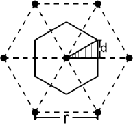
(a) A closer look at the neighborhood of a sensor node in a spatial distribution upon which the target distance function $H$ is based.

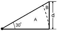
(b) A closer look at the shaded triangle in (a).

Figure 10: Geometric illustrations supporting the proof of Theorem A.1.

Given a 2-dimensional region of arbitrary shape, we know that perfectly circular regions covered by each sensor node (as assumed in the proof of Theorem II.1) will not achieve a space-filling tessellation of the area. Thus, the lower bounds on the quality of representation metrics will be higher for regions of arbitrary shape than those in Theorem  II.1. A 2-dimensional plane can achieve a regular symmetric tessellation with only three types of tiles: equilateral triangles, squares, or hexagons [41]. When an active sensor node is placed at the centroid of each tile, hexagonal tiles, being closer to a circular shape, achieve better quality of representation than triangles or squares. A region of interest of any arbitrary shape can achieve a space-filling tessellation with an infinite number of hexagonal tiles, each of infinitesimal size. Therefore, the quality of representation achieved by infinite space-filling hexagonal tiles, as shown in Fig.  4, is the best coverage that can be guaranteed for regions with an unknown arbitrary shape. The metrics $D(G,R)$ and $U(G,R)$ for this scenario represents, respectively, the upper bounds on the lower bounds of $D(G,R)$ and $U(G,R)$ for regions of arbitrary shape.

Let $r$ denote the distance between each pair of neighboring active sensor nodes (placed at the centroid of each hexagonal tile). Consider each of the innermost triangles (made up of dashed lines in Fig.  4) with sensor nodes as vertices. Consider the nodes near the center of the region (i.e., not at the boundary); each node belongs to six triangles and therefore, each triangle can be said to hold $3\times(1/6)=0.5$ nodes. Thus, given $z$ nodes per unit area, the number of these triangles that can cover a unit area is $z/0.5=2z$. Note that the area of each triangle is $\sqrt{3}r^{2}/4$. Since the area covered by $2z$ of these triangles is 1, we have $2z(\sqrt{3}r^{2}/4)=1$. Thus,

$$r=\sqrt{\frac{2}{\sqrt{3}z}}$$ (14)

For any point within each hexagonal tile, the closest sensor node is the one at the centroid of the tile. Since all the hexagonal tiles are congruent and identical with respect to the sensor node within them, $D(G,R)$ and $U(G,R)$ for the region of interest is the same as the $D(G,R)$ and $U(G,R)$ for any one hexagonal tile. Consider one such hexagonal tile, shown by solid lines in Fig.  10a. The hexagonal tile can be divided into twelve non-overlapping congruent right-angled triangles, one of which is shown shaded in Fig.  10a. Since the triangles are all congruent and also identical with respect to the placement of the nearest sensor node, $D(G,R)$ and $U(G,R)$ for the hexagonal cell is the same as the $D(G,R)$ and $U(G,R)$ for each triangle. Consider one such triangle, shown in Fig.  10b.

Denote by $d$ the length of the shortest edge of the triangle in Fig.  10b. Using elementary geometry, $d=\sqrt{3}r/6$. The triangular area can be divided into two parts:

• Area A: the area in which the distance between any point in the region to the sensor node is no larger than $\sqrt{3}d$.

• Area B: the area in which the distance between any point in the region to the sensor node is larger than $\sqrt{3}d$.

The two parts of the triangular region are shown in Fig.  10b. Thus, the expected distance between a point in the triangular area to the sensor node can be computed based on the expected distances from points within each of these two parts:

$$\overline{d} = \frac{\pi}{6}\int_{0}^{\sqrt{3}d}\frac{x^{2}dx}{\frac{\sqrt{3}}{2}d^{2}}+\int_{0}^{\frac{\pi}{6}}\int_{\sqrt{3}d}^{\frac{\sqrt{3}d}{sin(\theta+\frac{\pi}{3})}}\frac{x^{2}dxd\theta}{\frac{\sqrt{3}}{2}d^{2}}$$ (15)

$$= \left(\frac{2}{3}+\frac{1}{2}\ln 3\right)d$$

Given $d=\sqrt{3}r/6$ and Eqns.  (1) and  (14), we have:

$$D(G,R) = \overline{d}\sqrt{z}=\left(\frac{2}{3}+\frac{1}{2}\ln 3\right)d\sqrt{z}$$ (16)

$$= \left(\frac{1}{9}+\frac{1}{12}\ln 3\right)\sqrt{2\sqrt{3}}$$

$$\approx 0.3772$$

We now proceed to derive $U(G,R)$. Consider two random points whose distances to the sensor node are $x$ and $y$. There are three cases where the locations of the two points may fall.

• Case 1: Both points fall within Area A.

• Case 2: One of the points falls within Area A and the other within Area B.

• Case 3: Both points fall within Area B.

We now consider each of the three cases. In the following, $E_{w}[|x-y|]_{i}$ denotes the expected value of $|x-y|$ weighted by the probability of Case $i$.

Case 1:

$$E_{w}[|x-y|]_{1} = \int_{0}^{\sqrt{3}d}\int_{0}^{y}(y-x)\frac{\frac{\pi}{6}xdx}{\frac{\sqrt{3}}{2}d^{2}}\frac{\frac{\pi}{6}ydy}{\frac{\sqrt{3}}{2}d^{2}}$$ (17)

$$+ \int_{0}^{\sqrt{3}d}\int_{0}^{x}(x-y)\frac{\frac{\pi}{6}ydy}{\frac{\sqrt{3}}{2}d^{2}}\frac{\frac{\pi}{6}xdx}{\frac{\sqrt{3}}{2}d^{2}}$$

$$= \frac{\sqrt{3}{\pi}^{2}d}{45}$$

Case 2:

The probability that a point falls in Area A is

$$\int_{0}^{\sqrt{3}d}\frac{\frac{\pi}{6}xdx}{\frac{\sqrt{3}}{2}d^{2}}$$

and the probability that a point falls in area B is:

$$\int_{0}^{\frac{\pi}{6}}\int_{\sqrt{3}d}^{\frac{\sqrt{3}d}{\sin(\theta+\frac{\pi}{3})}}\frac{ydyd\theta}{\frac{\sqrt{3}}{2}d^{2}}$$

Define $k_{\theta}$ as:

$$k_{\theta}={\frac{\sqrt{3}d}{\sin(\theta+\frac{\pi}{3})}}$$

Therefore,

$$E_{w}[|x-y|]_{2} = 2\int_{0}^{\frac{\pi}{6}}\int_{\sqrt{3}d}^{k_{\theta}}\int_{0}^{\sqrt{3}d}(y-x)\frac{{\frac{\pi}{6}xdx}}{{\frac{\sqrt{3}}{2}d^{2}}}\frac{ydyd\theta}{\frac{\sqrt{3}}{2}d^{2}}$$ (18)

$$= \pi d(-\frac{2}{3}+\frac{2}{9}\sqrt{3}+\frac{1}{6}\sqrt{3}\ln 3)~{}~{}~{}~{}~{}~{}$$

Case 3:

The probability that both points fall in Area B is:

$$\left(\int_{0}^{\frac{\pi}{6}}\int_{\sqrt{3}d}^{\frac{\sqrt{3}d}{\sin(\theta+\frac{\pi}{3})}}\frac{ydyd\theta}{\frac{\sqrt{3}}{2}d^{2}}\right)^{2}$$

Define $k_{\eta}$ as:

$$k_{\eta}=\frac{\sqrt{3}d}{\sin(\eta+\frac{\pi}{3})}$$

Therefore,

$$E_{w}[|x-y|]_{3}=\int_{0}^{\frac{\pi}{6}}\int_{\sqrt{3}d}^{k_{\theta}}\int_{0}^{\frac{\pi}{6}}\int_{\sqrt{3}d}^{k_{\eta}}|x-y|\frac{dyd\eta}{\frac{\sqrt{3}}{2}d^{2}}\frac{dxd\theta}{\frac{\sqrt{3}}{2}d^{2}}$$ (19)

Since $E_{w}[|x-y|]_{3}$ is bounded above as follows:

$$E_{w}[|x-y|]_{3} < 2(\int_{0}^{\frac{\pi}{6}}\int_{\sqrt{3}d}^{k_{\theta}}\frac{ydyd\theta}{\frac{\sqrt{3}}{2}d^{2}})^{2}(2-\sqrt{3})$$

$$= 2(1-\frac{\sqrt{3}\pi}{6})^{2}(2-\sqrt{3})d$$

Thus, the overall expected difference between distances to the sensor node is:

$$E[|x-y|] = {E_{w}[|x-y|]}_{1}+{E_{w}[|x-y|]}_{2}+{E_{w}[|x-y|]}_{3}$$

$$< \frac{\sqrt{3}{\pi}^{2}d}{45}+\pi d(-\frac{2}{3}+\frac{2}{9}\sqrt{3}+\frac{1}{6}\sqrt{3}\ln 3)$$

$$+ 2(1-\frac{\sqrt{3}\pi}{6})^{2}(2-\sqrt{3})d$$

Using the above inequality with Eqns.  (1) and (15),

$$U(G,R)<0.2038$$

∎

Appendix B

In this section of the appendix, we consider $D(G,R)$ and $U(G,R)$ when the spatial distribution of active nodes is given by a Poisson point process.

Theorem B.1

If the spatial distribution of active nodes is given by a Poisson point process, the expected values of $D(G,R)$ and $U(G,R)$ are $0.5$ and $1-1/\sqrt{2}$, respectively.

Proof:

Consider active sensor nodes randomly distributed in the region of interest, $R$, given by a Poisson process of rate $z$ active nodes per unit area. Therefore, the probability that we will have $k$ nodes within some area $S$ is given by:

$$P(k,S)=\frac{(zS)^{k}e^{-zS}}{k!}$$ (20)

In the following, we assume that the region of interest is large enough to ignore boundary issues.

From Eqn.  (20), the probability that there are $0$ active nodes within a radius of $r$ is given by:

$$P(0,\pi r^{2})=\frac{(z\pi r^{2})^{0}e^{-z\pi r^{2}}}{(0)!}=e^{-z\pi r^{2}}$$ (21)

Consider a ring of radius $r$ of infinitesimal area equal to $2\pi rdr$. Using Eqn.  (20) again and noting that $2\pi rzdr\rightarrow 0$ implies $e^{-2\pi rzdr}\rightarrow 1-2\pi rzdr$, the probability that there is exactly one active node on this ring is given by:

$$P(1,2\pi rdr)=\frac{(2\pi rzdr)^{1}e^{-2\pi rz\,dr}}{1!}\approx 2\pi rz\,dr$$ (22)

Thus, the expected distance, $E[X_{1}]$, between the node and its nearest neighbor is given by:

$$E[X_{1}] = \int_{0}^{\infty}rP(0,\pi r^{2})P(1,2\pi rdr)$$ (23)

$$\approx \int_{0}^{\infty}re^{-z\pi r^{2}}2\pi rzdr$$

$$= \frac{1}{2\sqrt{z}}$$

Using Eqn.  (1), we get:

$$D(G,R)=\frac{1}{2}$$

We now derive the expected value of $U(G,R)$. Let $W$ denote a random variable indicating the distance of a random point from its nearest node. The probability density function of $W$ is given by:

$$p_{W}(r)=2\pi re^{-\pi r^{2}z}$$

Consider any two random points whose distances to their respective nearest nodes are $x$ and $y$. Now,

$$E[|x-y|] = \int_{0}^{\infty}p_{W}(x)\int_{0}^{\infty}p_{W}(y)|x-y|\,dy\,dx$$

$$= \int_{0}^{\infty}p_{W}(x)\int_{0}^{x}p_{W}(y)(x-y)\,dy\,dx$$

$$+ \int_{0}^{\infty}p_{W}(x)\int_{x}^{\infty}p_{W}(y)(y-x)\,dy\,dx$$

Focusing first on the inner integrals and simplifying, we get the following two results:

$$\int_{0}^{x}p_{W}(y)(x-y)dy = \int_{0}^{x}e^{-z\pi y^{2}}2\pi yz(x-y)dy$$ (24)

$$= x-\int_{0}^{x}e^{-z\pi y^{2}}dy$$

$$\int_{x}^{\infty}p_{W}(y)(y-x)dy = \int_{x}^{\infty}e^{-z\pi y^{2}}2\pi yzdy(y-x)dy$$ (25)

$$= \int_{x}^{\infty}e^{-z\pi y^{2}}dy$$

Define $g(x)$ as follows:

$$g(x)=\int_{0}^{x}e^{-z\pi y^{2}}dy$$

Since $g(\infty)=\frac{1}{2}\sqrt{\frac{1}{z}}$,

$$\int_{x}^{\infty}e^{-z\pi y^{2}}dy=\frac{1}{2}\sqrt{\frac{1}{z}}-g(x)$$

Using (24) and (25), $E[|x-y|]$ may be expressed as:

$$\int_{0}^{\infty}p_{W}(x)[x+\frac{1}{2}\sqrt{\frac{1}{z}}-2g(x)]dx$$

$$\approx \int_{0}^{\infty}e^{-z\pi x^{2}}2\pi xz\left[x+\frac{1}{2}\sqrt{\frac{1}{z}}-2g(x)\right]dx$$

$$= \sqrt{\frac{1}{z}}+2e^{-z\pi x^{2}}g(x)|_{0}^{\infty}-\int_{0}^{\infty}2e^{-z\pi x^{2}}\frac{d(g(x))}{dx}\,dx$$

Simplifying further using routine calculus, we get:

$$E[|x-y|]=\sqrt{\frac{1}{z}}(1-\sqrt{\frac{1}{2}})$$ (26)

Given that the expected distance to the nearest node is $1/2\sqrt{z}$, using Eqn.  (26) in the definition of $U(G,R)$, we get:

$$U(G,R)=\frac{1}{2\frac{1}{2}\sqrt{\frac{1}{z}}}\sqrt{\frac{1}{z}}(1-\sqrt{\frac{1}{2}})=1-\sqrt{\frac{1}{2}}$$

∎

References

- [1] I. F. Akyildiz, W. Su, Y. Sankarasubramaniam, and E. Cayirci, “A survey on sensor networks,” IEEE Communications Magazine, vol. 40, no. 8, pp. 102–114, Aug. 2002.
- [2] S. Meguerdichian, F. Koushanfar, M. Potkonjak, and M. B. Srivastava, “Coverage problems in wireless ad-hoc sensor networks,” in Proc. INFOCOM. IEEE, 2001, pp. 1380–1387.
- [3] C.-F. Huang and Y.-C. Tseng, “The coverage problem in a wireless sensor network,” Mob. Netw. Appl., vol. 10, no. 4, pp. 519–528, 2005.
- [4] B. Cărbunar, A. Grama, J. Vitek, and O. Cărbunar, “Redundancy and coverage detection in sensor networks,” ACM Trans. Sen. Netw., vol. 2, no. 1, pp. 94–128, 2006.
- [5] X. Y. Li, P. J. Wan, and O. Frieder, “Coverage in wireless ad hoc sensor networks,” IEEE Transactions on Computers, vol. 52, no. 6, pp. 753–763, Jun. 2003.
- [6] A. Gallais, J. Carle, D. Simplot-Ryl, and I. Stojmenovic, “Localized sensor area coverage with low communication overhead,” IEEE Transactions on Mobile Computing, vol. 7, no. 5, pp. 661–672, May 2008.
- [7] C. F. Huang, L. C. Lo, Y. C. Tseng, and W. T. Chen, “Decentralized energy-conserving and coverage-preserving protocols for wireless sensor networks,” ACM Trans. Sen. Netw., vol. 2, no. 2, pp. 182–187, 2006.
- [8] S. Shakkottai, R. Srikant, and N. Shroff, “Unreliable sensor grids: coverage, connectivity and diameter,” in Proc. INFOCOM. IEEE, 2003, pp. 1073–1083.
- [9] Crossbow Technology, Inc., “Motes, Smart Dust Sensors, WSNs,” 2009, http://www.xbow.com/.
- [10] IEEE, “IEEE 1451 smart transducer interface standards,” 2005. [Online]. Available: http://standards.ieee.org
- [11] D. Culler, D. Estrin, and M. Srivastava, “Overview of sensor networks,” IEEE Computer, vol. 37, no. 8, pp. 41–49, Aug. 2004.
- [12] J. Hill, R. Szewczyk, A. Woo, S. Hollar, D. E. Culler, and K. S. J. Pister, “System architecture directions for networked sensors.” in Proc. ACM SIGPLAN Notices. ACM, 2000, pp. 93–104.
- [13] D. Niculescu and B. Nath, “Ad hoc positioning system (APS) using AoA,” in Proc. INFOCOM. IEEE, 2003, pp. 1734–1743.
- [14] K. Krizman, T. E. Biedka, and T. S. Rappaport, “Wireless position location: Fundamentals, implementation strategies, and source of error,” in Proc. IEEE Vehicular Technology Conf. IEEE, 1997, pp. 919–923.
- [15] B. Raman and K. Chebrolu, “Censor networks: A critique of “sensor networks” from a systems perspective,” Computer Communication Review, vol. 38, no. 3, pp. 75–81, Jul. 2008.
- [16] Y.-C. Wang and Y.-C. Tseng, “Distributed deployment schemes for mobile wireless sensor networks to ensure multilevel coverage,” IEEE Transactions on Parallel and Distributed Systems, vol. 19, no. 9, pp. 1280–1294, 2008.
- [17] P. J. Clark and F. C. Evans, “Distance to nearest neighbor as a measure of spatial relationships in populations,” Ecology, vol. 35, no. 4, pp. 445–453, Oct. 1954.
- [18] A. Krause, C. Guestrin, A. Gupta, and J. Kleinberg, “Near-optimal sensor placements: maximizing information while minimizing communication cost,” in Proc. Int’l Conf. on Information Processing in Sensor Networks (IPSN). ACM, 2006, pp. 2–10.
- [19] F. A. Cowell, Measuring Inequality: Techniques for the Social Sciences. New York, NY, USA: John Wiley & Sons, New York, 1977.
- [20] A. W. Marshall and I. Olkin, Inequalities: Theory of Majorization and its Applications. New York, NY: Academic Press, New York, 1979.
- [21] D. Stoyan and H. Stoyan, Fractals, Random Shapes and Point Fields: Methods of Geometrical Statistics. Hoboken, NJ: John Wiley and Sons, 1994.
- [22] D. B. West, Introduction to Graph Theory. New Jersey, NJ: Prentice Hall, 2001.
- [23] A. J. O’Donnell and H. Sethu, “On achieving software diversity for improved network security using distributed coloring algorithms,” in Proc. ACM Conf. on Computer and Communications Security (CCS). ACM, 2004, pp. 121–131.
- [24] V. V. Vazirani, Approximation Algorithms. New York, NY: Springer-Verlag, 2001.
- [25] Z. Drezner and H. W. Hamacher, Facility Location: Applications and Theory. New York, NY: Springer, 2004.
- [26] S. H. Owen and M. S. Daskin, “Strategic facility location: A review,” European J. of Oper. Res., vol. 111, no. 3, pp. 423–447, Dec. 1998.
- [27] L. Qiu, V. N. Padmanabhan, and G. M. Voelker, “On the placement of web server replicas,” in Proc. INFOCOM. IEEE, 2001, pp. 1587–1596.
- [28] B. Li, M. J. Golin, G. F. Ialiano, and X. Deng, “On the optimal placement of web proxies in the Internet,” in Proc. INFOCOM. IEEE, 1999, pp. 1282–1290.
- [29] S. Kim, M. Yoon, and Y. Shin, “Placement algorithm of web server replicas,” in Lecture Notes in Comp. Sci., vol. 3043. Springer, 2004, pp. 328–336.
- [30] J. Kangasharju, J. Roberts, and K. W. Ross, “Object replication strategies in content distribution networks,” Computer Communication, vol. 25, no. 4, pp. 376–383, Mar. 2002.
- [31] B.-J. Ko and D. Rubenstein, “Distributed self-stabilizing placement of replicated resources in emerging networks,” IEEE/ACM Transactions on Networking, vol. 13, no. 3, pp. 476–487, Jun. 2005.
- [32] M. Cardei and D.-Z. Du, “Improving wireless sensor network lifetime through power-aware organization,” ACM Wireless Networks, vol. 11, no. 3, pp. 333–340, May 2005.
- [33] X. Chu and H. Sethu, “A new distributed algorithm for even coverage and improved lifetime in a sensor network,” in Proc. INFOCOM. IEEE, Apr. 2009, pp. 361–369.
- [34] J. Pach and P. K. Agarwal, Combinatorial Geometry, 3rd ed. New York, NY: Wiley-Interscience, 1995.
- [35] P. Brass, W. O. J. Moser, and J. Pach, Research Problems in Discrete Geometry. New York, NY: Springer, 2005.
- [36] S. M. N. Alam and Z. J. Haas, “Coverage and connectivity in three-dimensional networks,” in Proc. Int’l Conf. on Mobile Computing and Networking (MobiCom). ACM, 2006, pp. 346–357.
- [37] P. Santi, Topology Control in Wireless Ad Hoc and Sensor Networks. Hoboken, NJ: John Wiley and Sons, Ltd., 2006.
- [38] N. Li and J. C. Hou, “Localized topology control algorithms for heterogeneous wireless networks,” IEEE/ACM Transactions on Networking, vol. 13, no. 6, pp. 1313–1324, Dec. 2005.
- [39] H. Sethu and T. Gerety, “A new distributed topology control algorithm for wireless environments with non-uniform path loss and multipath propagation,” Ad Hoc Networks, vol. 8, no. 3, pp. 280–294, May 2010.
- [40] D. Tian and N. D. Georganas, “A coverage-preserving node scheduling scheme for large wireless sensor networks,” in Proc. Int’l Workshop on Wireless Sensor Networks and Applications. ACM, 2002, pp. 32–41.
- [41] L. C. Kinney and T. E. Moore, Symmetry, Shape and Space: An Introduction to Mathematics through Geometry. Emeryville, CA, USA: Key College Publishing, 2001.