Replica-Exchange Method in van der Waals Radius Space:
Overcoming Steric Restrictions for Biomolecules

Abstract

We present a new type of the Hamiltonian replica-exchange method, in which not temperatures but the van der Waals radius parameter is exchanged. By decreasing the van der Waals radii that control spatial sizes of atoms, this Hamiltonian replica-exchange method overcomes the steric restrictions and energy barriers. Furthermore, the simulation based on this method escapes from the local-minimum free-energy states and realizes effective sampling in the conformational space. We applied this method to an alanine dipeptide in aqueous solution and showed the effectiveness of the method by comparing the results with those obtained from the conventional canonical method.

I Introduction

Effective samplings in the conformational space by Monte Carlo (MC) and molecular dynamics (MD) simulations are necessary to predict the native structures of proteins. In the conventional canonical-ensemble simulations mrrtt53 ; hlm82 ; evans83 ; nose_mp84 ; nose_jcp84 ; hoover85 , however, it is difficult to realize effective samplings in complex systems such as proteins. This is because the usual canonical-ensemble simulations tend to get trapped in a few of many local-minimum states. To overcome these difficulties, various generalized-ensemble algorithms have been proposed (for reviews, see, e.g., Refs. mso01 ; ioo07 ).

The replica-exchange method (REM) hn96 is one of the most well-known methods among the generalized-ensemble algorithms (see Ref. so99 for the MD version). It is easier to implement than the multicanonical algorithm berg91 ; berg92 , which is also one of the most well-known generalized-ensemble algorithms (see Refs. hoe96 ; naka97 for the MD version), because we do not have to determine a probability weight factor in advance in the REM. In the multicanonical and similar algorithms oo04a ; oo04b ; oo04c ; oo04d ; oo06 ; berg03 ; itoh04 ; itoh06 ; itoh07a ; itoh07b we employ non-Boltzmann weight factors as the probability weight factors. These non-Boltzmann weight factors are not a priori known and have to be determined by tedious procedures. On the other hand, the usual Boltzmann weight factor is employed in REM, and therefore it is not necessary to determine the non-Boltzmann weight factor. The REM uses non-interacting replicas of the target system with different temperatures and realizes a random walk in temperature space by exchanging the temperatures of pairs of replicas. Accordingly, the simulation can avoid getting trapped in local-minimum free-energy states.

For large systems such as proteins in aqueous solution, however, the usual REM has a difficulty. We need to increase the number of replicas in proportion to $O(f^{\frac{1}{2}})$, where $f$ is the number of degrees of freedom hn96 . Large biomolecular systems, therefore, require a large number of replicas in the REM and hence huge amount of computation time. In order to overcome this difficulty, it was pointed out that the number of required replicas can be greatly decreased if only the parameter exchanges are performed in the multi-dimensional replica-exchange method (MREM) sko00 without temperature exchanges fwt02 . In MREM replica exchanges in temperature and/or parameter in the potential energy are performed. MREM is also referred to as the Hamiltonian replica-exchange method fwt02 , and in the present article we use the latter terminology.

When we perform simulations of a protein in explicit water solvent, most of the degrees of freedom is occupied by water molecules. In order to predict the native structure of a protein, for instance, we would like to sample effectively the conformational space of the protein rather than water molecules. As an application of the Hamiltonian REM, therefore, Berne and co-workers performed simulations of the peptide in explicit water solvent, in which the scales of the only interactions related to the protein are varied lkfb05 . They could achieve effective samplings in the conformational space of the peptide and saved CPU cost in comparison with the usual REM. Moreover, another application of the Hamiltonian REM was reported by Kannan and Zacharias kz07 . They focused on the backbone dihedral angles of the peptides and added biasing potential energy to the backbone dihedral angles. They could also achieve effective samplings in this space with the biasing potential energy. However, these biasing potential energy terms are complicated functions and highly dependent on force fields.

In this article, we propose a new type of Hamiltonian REM where we exchange the scaling factor of the van der Waals radius of solute atoms in the interaction terms among solute atoms only. By reducing this scaling factor, the steric hindrance among solute atoms will be reduced and wide conformational space can be explored. We applied this method to the sytems of an alanine dipeptide with explicit water molecules and tested the effectiveness of the method by comparing the results with those from the conventional canonical method.

In Section II we describe the new Hamiltonian REM. We give the details of the new Hamiltonian REM and canonical simulations that we performed in Section III. The results are presented in Section IV. Section V is devoted to conclusions.

II Methods

II.1 Hamiltonian REM

We first give a general formulation of the Hamiltonian REM sko00 .

We consider a system of N atoms with their coordinate vectors and momentum vectors denoted by $q\equiv\left\{{\mbox{\boldmath$q$}}_{1},\cdots,{\mbox{\boldmath$q$}}_{N}\right\}$ and $p\equiv\left\{{\mbox{\boldmath$p$}}_{1},\cdots,{\mbox{\boldmath$p$}}_{N}\right\}$, respectively. The Hamiltonian $H_{\lambda}$ in state $x\equiv(q,p)$ is given by the sum of the kinetic energy K and potential energy $E_{\lambda}$:

$$H_{\lambda}(x)=K(p)+E_{\lambda}(q)~{}.$$ (1)

Here, we are explicitly writing (or introducing) a parameter of interest in the potential energy as $\lambda$. In the canonical ensemble at temperature $T$, each state $x$ is weighted by the Boltzmann factor:

$$W_{\rm B}(x)=e^{-\beta H_{\lambda}(x)}~{},$$ (2)

where the inverse temperature $\beta$ is defined by $\beta=1/k_{\rm B}T$ ($k_{\rm B}$ is Boltzmann’s constant).

The generalized ensemble for the Hamiltonial REM consists of $M$ non-interacting copies (or, replicas) of the original system in the canonical ensemble at $M$ different parameter values $\lambda_{m}$ ($m=1,\cdots,M$). We arrange the replicas so that there is always exactly one replica at each $\lambda$ value. Then there is a one-to-one correspondence between replicas and parameter values; the label $i$ ($i=1,\cdots,M$) for replicas is a permutation of the label $m$ ($m=1,\cdots,M$) for $\lambda_{m}$, and vice versa:

$$\left\{\begin{array}[]{rl}i&=~{}i(m)~{}\equiv~{}f(m)~{},\cr m&=~{}m(i)~{}\equiv~{}f^{-1}(i)~{},\end{array}\right.$$ (3)

where $f(m)$ is a permutation function of $m$ and $f^{-1}(i)$ is its inverse.

Let $X=\left\{x_{1}^{[i(1)]},\cdots,x_{M}^{[i(M)]}\right\}=\left\{x_{m(1)}^{[1]},\cdots,x_{m(M)}^{[M]}\right\}$ stand for a “state” in this generalized ensemble. Here, the superscript $i$ and the subscript $m$ in $x_{m}^{[i]}$ label the replica and the parameter, respectively. The state $X$ is specified by the $M$ sets of coordinates $q^{[i]}$ and momenta $p^{[i]}$ of $N$ atoms in replica $i$ at parameter $\lambda_{m}$:

$$x_{m}^{[i]}\equiv\left(q^{[i]},p^{[i]}\right)_{m}~{}.$$ (4)

Because the replicas are non-interacting, the weight factor for the state $X$ in this generalized ensemble is given by the product of Boltzmann factors for each replica $i$ (or at each parameter $\lambda_{m}$):

$$W_{\rm HREM}(X)=\displaystyle{\prod_{i=1}^{M}}\displaystyle{\exp\left\{-\beta H_{\lambda_{m(i)}}\left(x_{m(i)}^{[i]}\right)\right\}}=\displaystyle{\prod_{m=1}^{M}}\displaystyle{\exp\left\{-\beta H_{\lambda_{m}}\left(x_{m}^{[i(m)]}\right)\right\}~{},}$$ (5)

where $i(m)$ and $m(i)$ are the permutation functions in Eq. (3).

We now consider exchanging a pair of replicas in the generalized ensemble. Suppose we exchange replicas $i$ and $j$ which are at parameter values $\lambda_{m}$ and $\lambda_{n}$, respectively:

$$X=\left\{\cdots,x_{m}^{[i]},\cdots,x_{n}^{[j]},\cdots\right\}\longrightarrow\ X^{\prime}=\left\{\cdots,x_{m}^{[j]},\cdots,x_{n}^{[i]},\cdots\right\}~{}.$$ (6)

The transition probability for this replica exchange process is given by the usual Metropolis criterion:

$$w(X\rightarrow X^{\prime})={\rm min}\left(1,\frac{W_{\rm HREM}(X^{\prime})}{W_{\rm HREM}(X)}\right)={\rm min}\left(1,\exp(-\Delta)\right)~{},$$ (7)

where we have sko00

$$\Delta=\beta\left[\left(E_{\lambda_{m}}\left(q^{[j]}\right)-E_{\lambda_{m}}\left(q^{[i]}\right)\right)-\left(E_{\lambda_{n}}\left(q^{[j]}\right)-E_{\lambda_{n}}\left(q^{[i]}\right)\right)\right]~{}.$$ (8)

Here, $q^{[i]}$ and $q^{[j]}$ stand for coordinate vectors for replicas $i$ and $j$, respectively, before the replica exchange. Note that we need to newly evaluate the potential energy for exchanged coordinates, $E_{\lambda_{m}}(q^{[j]})$ and $E_{\lambda_{n}}(q^{[i]})$, because $E_{\lambda_{m}}$ and $E_{\lambda_{n}}$ are in general different functions. We remark that the kinetic energy terms have canceled out each other in Eq. (8).

The Hamiltonian REM is realized by alternately performing the following two steps sko00 :

1. For each replica, a canonical MC or MD simulation at the corresponding parameter value $\lambda_{m}$ is carried out simultaneously and independently for a certain steps with the corresponding Boltzmann factor of Eq. (2) for each replica.

2. We exchange a pair of replicas $i$ and $j$ which are at the parameter values $\lambda_{m}$ and $\lambda_{n}$, respectively. The transition probability for this replica exchange process is given by Eqs. (7) and (8).

Finally, we remark that in order to further enhance sampling, we can always introduce a temperature-exchange process together with the above parameter exchange sko00 .

II.2 van der Waals Replica-Exchange Method

We now describe our special realization of the Hamiltonian REM, which we refer to as the van der Waals Replica-Exchange Method (vWREM).

We consider a system consisting of solute molecule(s) in explicit solvent. We can write the total potential energy as follows.

$$E_{\lambda}(q)=E_{\rm p}(q_{\rm p})+E_{\rm ps}(q_{\rm p},q_{\rm s})+E_{\rm s}(q_{\rm s})~{},$$ (9)

where $E_{\rm p}$ is the potential energy for the atoms in the solute only, $E_{\rm ps}$ is the interaction term between solute atoms and solvent atoms, and $E_{\rm s}$ is the potential energy for the atoms of the solvent molecules only. Here, $q=\{q_{\rm p},q_{\rm s}\}$, where $q_{\rm p}$ and $q_{\rm s}$ are the coordinate vectors of the solute atoms and the solvent atoms, respectively, and denoted by $q_{\rm p}\equiv\left\{{\mbox{\boldmath$q$}}_{1},\cdots,{\mbox{\boldmath$q$}}_{N_{\rm p}}\right\}$ and $q_{\rm s}\equiv\left\{{\mbox{\boldmath$q$}}_{N_{\rm p}+1},\cdots,{\mbox{\boldmath$q$}}_{N}\right\}$. ($N_{\rm p}$ is the total number of atoms in the solute.)

We are more concerned with effective sampling of the conformational space of the solute itself than that of the solvent molecules. The steric hindrance of the solute conformations are governed by the van der Waals radii of each atom in the solute. Namely, when the van der Waals radii are large, the solute molecule is bulky and we have more steric hindrance among the solute atoms by the Lennard-Jones interactions, and when it is small, the solute molecule can move more freely. We thus introduce a parameter $\lambda$ that scales the van der Waals radius of each atom in the solute by

$$\sigma_{k\ell}\longrightarrow\lambda\sigma_{k\ell}~{},$$ (10)

and write the Lennard-Jones energy term within $E_{\rm p}$ in Eq. (9) as follows:

$$V_{\lambda}\left(q_{\rm p}\right)=\sum^{N_{\rm p}-1}_{k=1}\sum^{N_{\rm p}}_{\ell=k+1}4{\epsilon_{k\ell}}\left\{\left(\frac{\lambda\sigma_{k\ell}}{r_{k\ell}}\right)^{12}-\left(\frac{\lambda\sigma_{k\ell}}{r_{k\ell}}\right)^{6}\right\}~{},$$ (11)

where $r_{k\ell}$ is the distance between atoms $k$ and $\ell$ in the solute and $\epsilon_{k\ell}$ and $\sigma_{k\ell}$ are the corresponding Lennard-Jones parameters. The original potential energy is recovered when $\lambda=1$, and the steric hindrance of solute conformations is reduced when $\lambda<1$. Note that this is the only $\lambda$-dependent term in $E_{\lambda}$ in Eq. (9).

We prepare $M$ values of $\lambda$, $\lambda_{m}$ ($m=1,\cdots,M$). Without loss of generality, we can assume that the parameter values are ordered as $\lambda_{1}<\cdots<\lambda_{M}$. The vWREM is realized by alternately performing the following two steps:

1. For each replica, a canonical MC or MD simulation at the corresponding parameter value $\lambda_{m}$ is carried out simultaneously and independently for a certain steps with the corresponding Boltzmann factor of Eq. (2) for each replica.

2. We exchange a pair of replicas $i$ and $j$ which are at the neighboring parameter values $\lambda_{m}$ and $\lambda_{m+1}$, respectively. The transition probability for this replica exchange process is given by Eq. (7), where $\Delta$ in Eq. (8) now reads

   $$\Delta=\beta\left[\left(V_{\lambda_{m}}\left(q^{[j]}_{\rm p}\right)-V_{\lambda_{m}}\left(q^{[i]}_{\rm p}\right)\right)-\left(V_{\lambda_{m+1}}\left(q^{[j]}_{\rm p}\right)-V_{\lambda_{m+1}}\left(q^{[i]}_{\rm p}\right)\right)\right]~{}.$$ (12)

   Here, $V_{\lambda}$ is the Lennard-Jones potential energy in in Eq. (11) among the solute atoms only.

Note that because the $\lambda$ dependence of $E_{\lambda}$ exists only in $V_{\lambda}$, the rest of the terms have been cancelled out in Eq. (8).

We see that Eq. (12) includes only the coordinates $q_{\rm p}$ of the atoms in the solute only and is independent of the coordinates $q_{\rm s}$ of solvent molecules. Because $N_{\rm p}\ll N$ usually holds, the difficulty in the usual REM that the number of required replicas increases with the number of degrees of freedom is much alleviated in this formalism.

II.3 Reweighting Techniques

The results from Hamiltonian REM simulations with different parameter values can be analyzed by the reweighting techniques fs89 ; kbskr92 . Suppose that we have carried out a Hamiltonian REM simulation at a constant temperature $T_{0}$ with $M$ replicas corresponding to $M$ parameter values $\lambda_{m}$ ($m=1,\cdots,M$).

For appropriate reaction coordinates $\xi_{1}$ and $\xi_{2}$, the canonical probability distribution $P_{T,\lambda}(\xi_{1},\xi_{2})$ with any parameter value $\lambda$ at any temperature $T$ can be calculated from

$$P_{T,\lambda}(\xi_{1},\xi_{2})=\sum_{E_{\lambda_{1}},\cdots,E_{\lambda_{M}}}\frac{\displaystyle\sum^{M}_{m=1}\left(g_{m}\right)^{-1}N_{m}(E_{\lambda_{1}},\cdots,E_{\lambda_{M}};\xi_{1},\xi_{2})e^{-\beta E_{\lambda}}}{\displaystyle\sum^{M}_{m=1}\left(g_{m}\right)^{-1}n_{m}e^{f_{T_{0},\lambda_{m}}-\beta_{0}E_{\lambda_{m}}}}~{},$$ (13)

and

$$e^{-f_{T_{0},\lambda_{m}}}=\sum_{\xi_{1},\xi_{2}}P_{T_{0},\lambda_{m}}(\xi_{1},\xi_{2})~{}.$$ (14)

Here, $g_{m}=1+2\tau_{m}$, $\tau_{m}$ is the integrated autocorrelation time with the parameter value $\lambda_{m}$ at temperature $T_{0}$, $N_{m}(E_{\lambda_{1}},\cdots,E_{\lambda_{M}};\xi_{1},\xi_{2})$ is the histogram of the $M$-dimensional energy distributions at the parameter value $\lambda_{m}$ and the reaction coordinate values $(\xi_{1},\xi_{2})$, which was obtained by the Hamiltonian REM simulation, $n_{m}$ is the total number of samples obtained at the parameter value $\lambda_{m}$. Note that this probability distribution is not normalized. Equations (13) and (14) are solved self-consistently by iteration. For biomolecular systems the quantity $g_{m}$ can safely be set to be a constant in the reweighting formulas kbskr92 , and so we set $g_{m}=1$ throughout the analyses in the present work. Note also that these equations can be easily generalized to any reaction coordinates $(\xi_{1},\xi_{2},\cdots)$.

¿From the probability distribution $P_{T,\lambda}(\xi_{1},\xi_{2})$ in Eq. (13), the expectation value of a physical quantity $A$ with any parameter value $\lambda$ at any temperature $T$ is given by

$$\left<A\right>_{T,\lambda}=\frac{\displaystyle\sum_{\xi_{1},\xi_{2}}A(\xi_{1},\xi_{2})P_{T,\lambda}(\xi_{1},\xi_{2})}{\displaystyle\sum_{\xi_{1},\xi_{2}}P_{T,\lambda}(\xi_{1},\xi_{2})}~{}.$$ (15)

We can also calculate the free energy (or, the potential of mean force) as a function of the reaction coordinates $\xi_{1}$ and $\xi_{2}$ with any parameter value $\lambda$ at any temperature $T$ from

$$F_{T,\lambda}(\xi_{1},\xi_{2})=-k_{\rm B}T{\rm ln}{P_{T,\lambda}(\xi_{1},\xi_{2})}~{}.$$ (16)

By utilizing these equations, therefore, we can obtain various physical quantities from the Hamiltonian REM simulations with the original and non-original parameter values. We remark that although we wrote any $T$ in Eqs. (13), (15), and (16) above, the valid value $T$ is limited in the vicinity of $T_{0}$. We also need the $T$-exchange process in order to have accurate average quantities for a wide range of $T$ values.

III Computational Details

In order to demonstrate the effectiveness of the present Hamiltonian REM, namely, vWREM, in which we exchange pairs of the van der Waals radius parameter values, we applied the vWREM MD algorithm, which we refer to as the vWREMD, to the system of an alanine dipeptide in explicit water solvent and compared the results with those obtained by the conventional canonical MD simulation. The N-terminus and the C-terminus were blocked by the acetyl group and the N-methyl group, respectively. The number of water molecules was 67. The force field that we adopted was the AMBER parm96 parameter set amber96 , and the model for the water molecules was the TIP3P rigid-body model tip3p . The vWREMD and canonical MD simulations were carried out with the symplectic integrator with rigid-body water molecules, in which the temperature was controlled by the Nosé-Poincaré thermostat bll99 ; nose01 ; oio07 ; oo07 ; oo08 ; o08 . The system was put in a cubic unit cell with the side length of 13.4 Å, and we imposed the periodic boundary conditions. The electrostatic potential energy was calculated by the Ewald method, and we employed the minimum image convention for the Lennard-Jones potential energy. The time step was taken to be 0.5 fs.

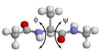
Figure 1: The common initial conformation of the alanine dipeptide. The figure was created with RasMol rasmol .

In the vWREMD simulation, we needed only four replicas ($M=4$). That is, we employed four different parameter values $\lambda_{m}$ $(m=1,\cdots,4)$. In Table 1 we list the values of these parameters. The original potential energy corresponds to the scale factor $\lambda_{4}=1.0$, and in the canonical MD simulation we employed this original parameter value of 1.0, The temperature of the system $T_{0}$ was set to be 300 K for all the replicas in the vWREMD and in the canonical MD simulation. Moreover, the initial conformations were also the same for all the simulations, and the initial backbone dihedral angles $\phi$ and $\psi$ of the alanine dipeptide were set $(\phi,\psi)=(180^{\circ},180^{\circ})$ as shown in Fig. 1. The total time of the MD simulations were 2.5 ns per replica for the vWREMD simulation and 2.5 ns for the canonical simulation, including equilibration for 0.1 ns. The trajectory data were stored every 50 fs. The replica exchange was tried every 250 fs in the vWREMD simulation.

IV Comparisons of the vWREMD simulation with the canonical MD simulation

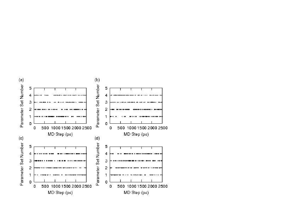
Figure 2: Time series of the label $m$ of the parameter $\lambda_{m}$ ($m=1,2,3,4$) in (a) Replica 1, (b) Replica 2, (c) Replica 3, and (d) Replica 4 during the vWREMD simulation.

We first examine whether the exchanges of pairs of the parameter values were realized sufficiently in our vWREMD simulation. In Table 2 we list the acceptance ratios of replica exchange of the parameter values in the vWREMD simulation. These acceptance ratios are large enough ($>$ 40 $\%$) except for the pair of $\lambda_{4}$ and $\lambda_{1}$. Because the difference of these parameter values is much larger than those of other pairs, this low acceptance ratio is expected, and it does not affect the REM performance. Figure 2 shows the time series of the parameter set number $m$ in $\lambda_{m}$ which each replica visited. This figure shows that random walks in the parameter space were realized in the vWREMD simulation.

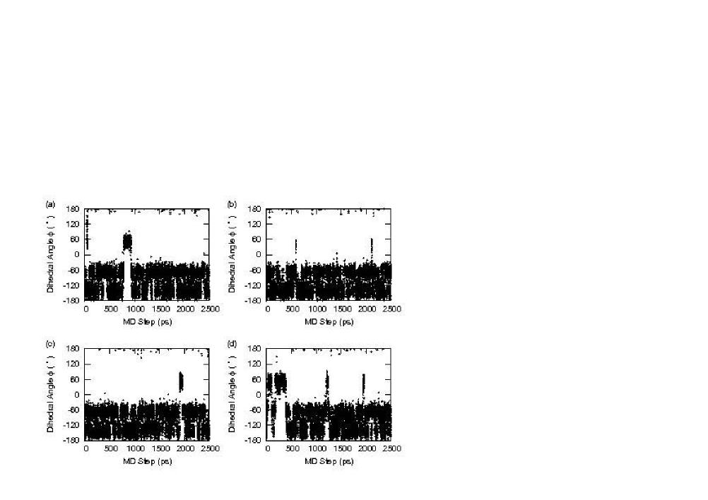
Figure 3: Time series of the dihedral angles $\phi$ in (a) Replica 1, (b) Replica 2, (c) Replica 3, and (d) Replica 4 during the vWREMD simulation.

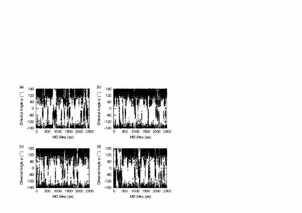
Figure 4: Time series of the dihedral angles $\psi$ in (a) Replica 1, (b) Replica 2, (c) Replica 3, and (d) Replica 4 during the vWREMD simulation.

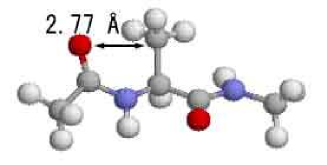
Figure 5: The snapshot of the alanine dipeptide at 2,469 ps in Replica 3 in the vWREMD simulation. The distance between the ${\rm C}_{\beta}$ atom of the alanine and the O atom of the acetyl group is presented. The figure was created with RasMol rasmol .

Figures 3 and 4 show the time series of the backbone-dihedral angles $\phi$ and $\psi$ for each replica. Figure 3 indicates that it is difficult to sample the range of the dihedral angle $\phi$ between $90^{\circ}$ and $180^{\circ}$. This is because the steric restriction between the ${\rm C}_{\beta}$ atom of the alanine and the O atom of the acetyl group prevent the rotation in this range. For instance, Fig. 5 is the snapshot of the alanine dipeptide which corresponds to the structure at 2,469 ps in Replica 3. In this structure the angle $\phi$ is $148.8^{\circ}$, and the distance between the ${\rm C}_{\beta}$ atom of the alanine and the O atom of the acetyl group is 2.77 Å. For such a short distance, the two atoms collide with each other. Therefore, the sampling among the range of $90^{\circ}<\phi<180^{\circ}$ in the vWREMD simulation was rare, although the scale factor $\lambda_{m}$ for the van der Waals radii was lessened. In order to sample this range frequently, it is necessary to employ a much smaller scale factor than the present case. However, conformations among this range have quite high potential energy due to the collisions between the ${\rm C}_{\beta}$ atom of the alanine and the O atom of the acetyl group, and it is not so important to sample this range at room temperature. On the other hand, the vWREMD simulation realized effective samplings with respect to $\psi$ in all the replicas as shown in Fig. 4. This is because the van der Waals radius of the H atom of the N-methyl group that have the covalent bond with the N atom of the N-methyl group is small, and steric restrictions between the ${\rm C}_{\beta}$ atom of the alanine and the H atom are less than those between the ${\rm C}_{\beta}$ atom of the alanine and the O atom of the acetyl group.

Figures 6 and 7 show the time series of the backbone-dihedral angles $\phi$ and $\psi$ for each parameter value. For comparisons, we also show those from the conventional MD simulation with the original parameter value of $\lambda=1$. These figures show that the smaller the scale factor $\lambda_{m}$ of the van der Waals radii is, the more efficient the sampling in the backbone-dihedral-angle space is. This is because the steric restrictions are reduced by lessening the scale factor and the energy barriers caused by the steric restrictions are decreased. Comparing Fig. 6(d) with Fig. 6(e) and Fig. 7(d) with Fig. 7(e), moreover, the vWREMD with the original parameter value $\lambda_{4}$ sampled the dihedral-angle space more effectively than the usual canonical MD simulation and did not get trapped in the local-minimum free-energy states. In other words, the canonical MD simulation with the original parameter value could not overcome energy barriers caused by the steric restrictions and got trapped in the local-minimum free-energy states. Therefore, effective samplings in the dihedral-angle space cannot be realized in the usual canonical MD simulations.

The logarithm of the probability distributions, ${\rm ln}P(\phi,\psi)$, with respect to dihedral angles $\phi$ and $\psi$ were obtained from the vWREMD simulations. Figures 8 and 9 show ${\rm ln}P(\phi,\psi)$ for each replica and those for each parameter value, respectively. From Fig. 8 we see that there are two regions in the vicinites of $(\phi,\psi)=(0^{\circ},0^{\circ})$ and $(\phi,\psi)=(0^{\circ},180^{\circ})$ in which the samplings were rare except the range of $90^{\circ}<\phi<180^{\circ}$. This is because in the vicinity of $(\phi,\psi)=(0^{\circ},0^{\circ})$, the O atom of the acetyl group and the H atom of N-methyl group collide with each other as in a structure shown in Fig. 10(a). In the region of the neighborhood of $(\phi,\psi)=(0^{\circ},180^{\circ})$, the O atom of the acetyl group and the O atom of the alanine also collide as in a structure shown in Fig. 10(b). It is obvious that steric restrictions in these regions were reduced and that the energy barriers were decreased by decreasing the scale factor as shown in Fig. 9. However, the effects of reducing energy barriers around $(\phi,\psi)=(0^{\circ},180^{\circ})$ are less than those around $(\phi,\psi)=(0^{\circ},0^{\circ})$. This is because the O atom of the acetyl group and the O atom of the alanine have negative charges, and repulsive forces caused by these charges act on both atoms. Therefore, by reducing the atomic charges as well as the van der Waals radii, more effective sampling may be realized in the conformational space.

Figure 11 shows the free-energy landscapes at $T_{0}=300$ K with respect to the backbone-dihedral angles $\phi$ and $\psi$ with the original parameter value ($\lambda=1$). The free-energy landscape in Fig. 11(a) was calculated from Eq. (16) by the reweighting techniques in Eqs. (13) and (14). The free-energy landscapes in Fig. 11(b) and Fig. 11(c) were obtained from the raw histogram with the original parameter value $\lambda_{4}$ in the vWREMD simulation and the raw histogram in the canonical MD simulation, respectively. The free-energy landscape of the conventional canonical MD simulation is inaccurate due to insufficient sampling in the backbone-dihedral-angle space as shown in Figs. 6(e) and 7(e). The free-energy landscape obtained by the reweighting techniques in Fig. 11(a) shows a better statistics even at free-energy barriers among the local-minimum states in comparison with that obtained from the raw histogram in Fig. 11(b). This is because the information of all the other parameter values can be reflected by the reweighting techniques. Therefore, more accurate free-energy landscape can be obtained by the reweighting techniques.

V Conclusions

In this article, we introduced a new type of Hamiltonian REM, the van der Waals REM (vWREM) in which the scale factor of the van der Waals radii of the solute atoms is exchanged only in the Lennard-Jones interactions among themselves. The steric hindrance due to the Lennard-Jones repulsions can be reduced by this method. Accordingly, the vWREM simulation can realize effective sampling in the backbone-dihedral-angle space without getting trapped in local-minimum free-energy states in comparison with the conventional canonical MD simulation. Employing the reweighting techniques, furthermore, we can obtain accurate free-energy landscape.

Although we considered only exchanges of the scale factor of the van der Waals radii in this article, this idea can be extended to other parameters. For example, the scale factor of partial charges of solute atoms so that we can also realize even more efficient sampling in the conformational space. The generalization of the formalism in Sec. II to other parameters is straightforward including the reweighting techniques. Moreover, these formalisms are independent of the degrees of freedom of solvent molecules. Therefore, these algorithms can be easily applied to large biomolecular systems.

Table 1: The values of the scaling factor, $\lambda_{m}$ ($m=1,\cdots,4$), of the van der Waals radii in the vWREMD simulation.

Parameter $\lambda_{m}$	Parameter value
$\lambda_{1}$	0.85
$\lambda_{2}$	0.90
$\lambda_{3}$	0.95
$\lambda_{4}$	1.00

Table 2: Acceptance ratios of replica exchange between pairs of the neighboring parameter values.

Pair of parameter values	Acceptance ratio
$\lambda_{1}$ $\leftrightarrow$ $\lambda_{2}$	0.482
$\lambda_{2}$ $\leftrightarrow$ $\lambda_{3}$	0.540
$\lambda_{3}$ $\leftrightarrow$ $\lambda_{4}$	0.442
$\lambda_{4}$ $\leftrightarrow$ $\lambda_{1}$	0.055

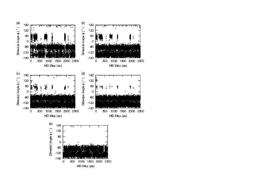
Figure 6: Time series of the dihedral angle $\phi$ with the parameter values (a) $\lambda_{1}$, (b) $\lambda_{2}$, (c) $\lambda_{3}$, and (d) $\lambda_{4}$ during the vWREMD simulation. (e) Time series of the dihedral angle $\phi$ during the conventional canonical MD simulation.

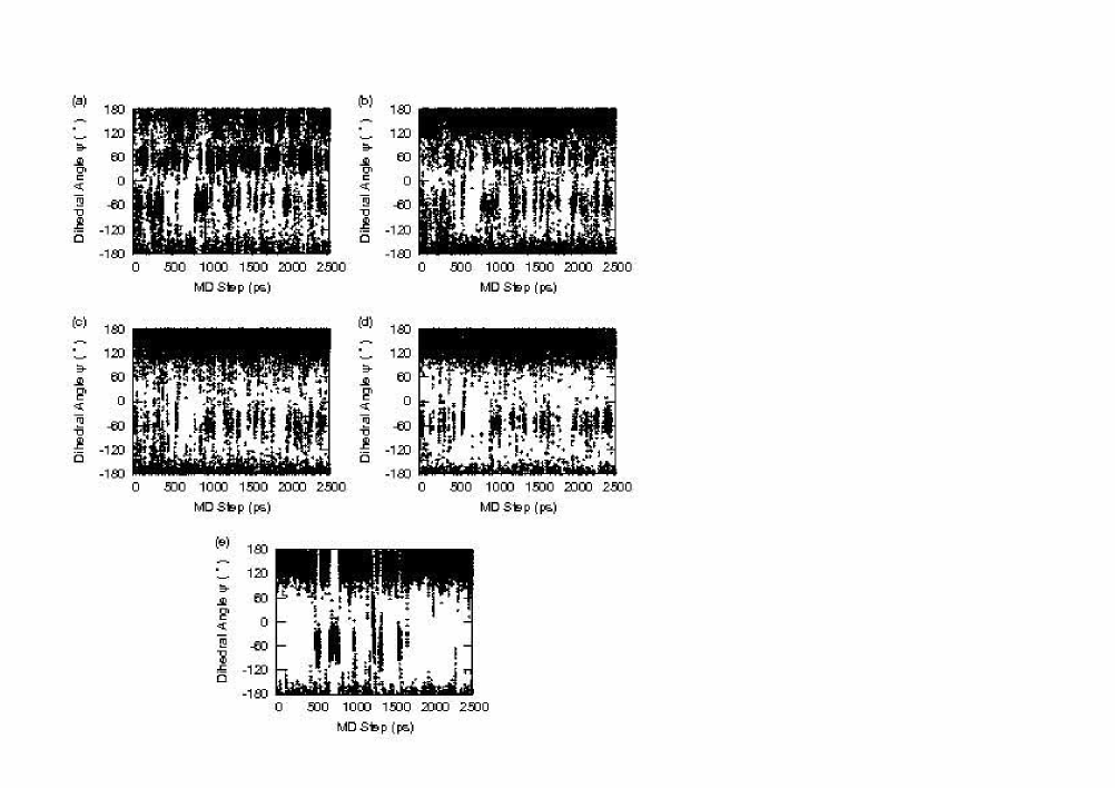
Figure 7: Time series of the dihedral angle $\psi$ with the parameter values (a) $\lambda_{1}$, (b) $\lambda_{2}$, (c) $\lambda_{3}$, and (d) $\lambda_{4}$ during the vWREMD simulation. (e) Time series of the dihedral angle $\psi$ during the conventional canonical MD simulation.

Figure 8: The logarithm of the probability distribution ${\rm ln}P(\phi,\psi)$ with respect to the dihedral angles $\phi$ and $\psi$ for (a) Replica 1, (b) Replica 2, (c) Replica 3, and (d) Replica 4 in the vWREMD simulation.

Figure 9: The logarithm of the probability distribution ${\rm ln}P(\phi,\psi)$ with respect to the dihedral angles $\phi$ and $\psi$ with parameter values (a) $\lambda_{1}$, (b) $\lambda_{2}$, (c) $\lambda_{3}$, and (d) $\lambda_{4}$ in the vWREMD simulation.

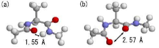
Figure 10: (a) The snapshot of the alanine dipeptide at 895.55 ps in Replica 1 in the vWREMD simulation. The structure has backbone-dihedral angles of $(\phi,\psi)=(15.5^{\circ},5.2^{\circ})$. The distance between the O atom of the acetyl group and the H atom of N-methyl group is given. (b) The snapshot of the alanine dipeptide at 2,465.65 ps in Replica 1 in the vWREMD simulation. The structure has backbone-dihedral angles of $(\phi,\psi)=(-27.7^{\circ},174.1^{\circ})$. The distance between the O atom of the acetyl group and the O atom of the alanine is given. The figures were created with RasMol rasmol .

Figure 11: The free-energy landscapes at $T_{0}=300$ K with respect to the backbone-dihedral angles $\phi$ and $\psi$ with the original parameter value $\lambda=1$. These were obtained from (a) the reweighting techniques applied to the results of the vWREMD simulation, (b) the raw histogram with the original parameter value $\lambda_{4}$ in the vWREMD simulation, and (c) the raw histogram in the canonical MD simulation.

References

- (1) N. Metropolis, A. W. Rosenbluth, M. N. Rosenbluth, A. H. Teller, and E. Teller, J. Chem. Phys. 21, 1087 (1953).
- (2) W. G. Hoover, A. J. C. Ladd, and B. Moran, Phys. Rev. Lett. 48, 1818 (1982).
- (3) D. J. Evans, J. Chem. Phys. 78, 3297 (1983).
- (4) S. Nosé, Mol. Phys. 52, 255 (1984).
- (5) S. Nosé, J. Chem. Phys. 81, 511 (1984).
- (6) W. G. Hoover, Phys. Rev. A 31, 1695 (1985).
- (7) A. Mitsutake, Y. Sugita, and Y. Okamoto, Biopolymers (Peptide Science) 60, 96 (2001).
- (8) S. G. Itoh, H. Okumura, and Y. Okamoto, Mol. Sim. 33, 47 (2007).
- (9) K. Hukushima and K. Nemoto, J. Phys. Soc. Jpn. 65, 1604 (1996).
- (10) Y. Sugita and Y. Okamoto, Chem. Phys. Lett. 314, 141 (1999).
- (11) B. A. Berg and T. Neuhaus, Phys. Lett. B267, 249 (1991).
- (12) B. A. Berg and T. Neuhaus, Phys. Rev. Lett. 68, 9 (1992).
- (13) U. H. E. Hansmann, Y. Okamoto, and F. Eisenmenger, Chem. Phys. Lett. 259, 321 (1996).
- (14) N. Nakajima, H. Nakamura, and A. Kidera, J. Phys. Chem. B 101, 817 (1997).
- (15) H. Okumura and Y. Okamoto, Chem. Phys. Lett. 383, 391 (2004).
- (16) H. Okumura and Y. Okamoto, Phys. Rev. E 70, 026702 (2004).
- (17) H. Okumura and Y. Okamoto, J. Phys. Soc. Jpn. 73, 3304 (2004).
- (18) H. Okumura and Y. Okamoto, Chem. Phys. Lett. 391, 248 (2004).
- (19) H. Okumura and Y. Okamoto, J. Comput. Chem. 27, 379 (2006).
- (20) B. A. Berg, H. Noguchi, and Y. Okamoto, Phys. Rev. E 68, 036126 (2003).
- (21) S. G. Itoh and Y. Okamoto, Chem. Phys. Lett. 400, 308 (2004).
- (22) S. G. Itoh and Y. Okamoto, J. Chem. Phys. 124, 104103 (2006).
- (23) S. G. Itoh and Y. Okamoto, Mol. Sim. 33, 83 (2007).
- (24) S. G. Itoh and Y. Okamoto, Phys. Rev. E 76, 026705 (2007).
- (25) Y. Sugita, A. Kitao, and Y. Okamoto, J. Chem. Phys. 113, 6042 (2000).
- (26) H. Fukunishi, O. Watanabe, and S. Takada, J. Chem. Phys. 116, 9058 (2002).
- (27) P. Liu, B. Kim, R .A. Friesner, and B. J. Berne, Proc. Natl. Acad. Sci. USA 102, 13749 (2005).
- (28) S. Kannan and M. Zacharias, Proteins 66, 697 (2007).
- (29) A. M. Ferrenberg and R. H. Swendsen, Phys. Rev. Lett. 63, 1195 (1989).
- (30) S. Kumar, D. Bouzida, R. H. Swendsen, P. A. Kollman, and J. M. Rosenberg, J. Comput. Chem. 13, 1011 (1992).
- (31) P. A. Kollman, R. Dixon, W. Cornell, T. Fox, C. Chipot, and A. Pohorille, in “Computer Simulation of Biomolecular Systems, Vol 3,” ed. by A. Wilkinson, P. Weiner, W. F. van Gunsteren, (Elsevier, Dordrecht, 1997) p. 83.
- (32) W. L. Jorgensen, J. Chandrasekhar, J. D. Madura, R. W. Impey, and M. L. Klein, J. Chem. Phys. 79, 926 (1983).
- (33) S. D. Bond, B. J. Leimkuhler, and B. B. Laird, J. Comput. Phys. 151, 114 (1999).
- (34) S. Nosé, J. Phys. Soc. Jpn. 70, 75 (2001).
- (35) H. Okumura, S. G. Itoh, and Y. Okamoto, J. Chem. Phys. 126, 084103 (2007).
- (36) H. Okumura and Y. Okamoto, Bull. Chem. Soc. Jpn. 80, 1114 (2007).
- (37) H. Okumura and Y. Okamoto, J. Phys. Chem. B 112, 12038 (2008).
- (38) H. Okumura, J. Chem. Phys. 129, 124116 (2008).
- (39) R. A. Sayle and E. J. Milner-White, Trends Biochem. Sci. 20, 374 (1995).