Realistic Flipped SU(5) from Orbifold SO(10)

Abstract:

We propose a realistic flipped $SU(5)$ model derived from a five-dimensional orbifold $SO(10)$ model. The Standard Model (SM) fermion masses and mixings are explained by combining the traditional Froggatt-Nielsen mechanism with the five-dimensional wave function profiles of the SM fermions. Employing tree-level spontaneous R-symmetry breaking in the hidden sector and extra(ordinary) gauge mediation, we obtain realistic supersymmetry breaking soft mass terms with non-vanishing gaugino masses. Including the messenger fields at the intermediate scale and Kaluza-Klein states at the compactification scale, we study gauge coupling unification. We show that the $SO(10)$ unified gauge coupling is very strong and the unification scale can be much higher than the compactification scale. We briefly discuss proton decay as well.

1 Introduction

As one of the most attractive extensions of the Standard Model (SM), supersymmetric Grand Unification Theories (GUTs) like $SU(5)$ [1] or $SO(10)$ [2] give us deep insights into the problems such as charge quantization, neutrino masses and mixings as well as the origin of the Yukawa sector. However, these theories still have some unsatisfactory features such as the doublets-triplet (D-T) splitting problem, rapid proton decay, and unrealistic SM fermion mass relations, etc.

The $SO(10)$ models are pretty interesting since they have both the gauge interaction unification and the SM fermion unification. One type of these models, where the gauge symmetry is broken down to the Georgi-Glashow $SU(5)$, have the rapid proton decay and D-T splitting problems in the subsequent gauge symmetry breaking into the SM. In contrast, another type with symmetry breaking to flipped $SU(5)$ might be more attractive because the flipped $SU(5)$ models can solve the D-T splitting problem via missing partner mechanism as well as the dimension-five proton decay problem [3, 4, 5]. Although embedding flipped $SU(5)$ into $SO(10)$ can retrieve gauge unification, the missing partner mechanism does not work in four-dimensional models (for a possible solution, see Ref. [6]). A simple solution is to realize such embedding in five-dimensional orbifold. Orbifold GUT models for $SU(5)$ were proposed in [7, 8, 9] and widely studied thereafter in [10, 11, 12, 13, 14, 15, 16, 17, 18]. Orbifold $SO(10)$ models with symmetry breaking to Pati-Salam models were studied in [19, 20]. And earlier studies on orbifold $SO(10)$ models with symmetry breaking to flipped $SU(5)$ can be found in [21, 22].

In this paper we consider a realistic flipped $SU(5)$ model derived from the five-dimensional orbifold $SO(10)$ and study its phenomenological consequence. As we know, it is interesting to explain the SM fermion masses and mixings in the Minimal Supersymmetric Standard Model (MSSM) from the top-down approach. In particular, the Froggat-Nielson mechanism [23] can be very predictive in the GUTs. The efforts to explain the flavor structure through the deformed Froggat-Nielson mechanism in orbifold $SU(5)$ models were shown in [24, 25, 26], in which the SM fermion mass and mixing hierarchies are obtained via wave-function profiles of the SM fermions by adding bulk mass terms [27]. However, we find that in the flipped $SU(5)$ model it is not as simple as in the ordinary $SU(5)$ model to explain the SM fermion masses and mixings by such Froggat-Nielson mechanism because of the flipping of the right-handed up- and down-type quarks. Besides, the neutrino masses and mixings obtained from double see-saw mechanism set stringent constraints on the possible quark mass hierarchies in the flipped $SU(5)$ model. Therefore, we will introduce an additional discrete $Z_{3}$ symmetry, and combine the traditional Froggat-Nielsen mechanism with the wave-function profiles of the SM fermions. In this way we can generate the observed SM fermion masses and mixings.

In addition, we will discuss the relevant problems on supersymmetry (SUSY) breaking. We use the tree-level spontaneously R-symmetry breaking model and (extra)ordinary gauge mediation to obtain the realistic SUSY breaking soft mass terms with non-vanishing gaugino masses, which is in contrast to the previous models with vanishing gaugino masses by direct gauge mediation. Moreover, by including the messenger fields at the intermediate scale and the Kaluza-Klein (KK) states at the compactification scale, we will study the gauge coupling unification in details. Our study shows that the $SO(10)$ unified gauge coupling is very strong, and the unification scale can be much higher than the compactification scale. We will also comment on the proton decay.

This paper is organized as follows. In Section 2 we recapitulate the flipped $SU(5)$ model. In Section 3 we present the orbifold $SO(10)$ models where the gauge symmetry is broken down to the flipped $SU(5)$. In Section 4 we explain the SM fermion masses and mixings via the usual Froggat-Nielson mechanism and wave function profiles of the SM fermions. In Section 5 we discuss the four-dimensional $N=1$ supersymmetry breaking via the tree-level spontaneously R-symmetry breaking in hidden sector and (extra)ordinary gauge mediation. In Section 6 we discuss the strongly coupled gauge coupling unification with the threshold corrections from the messenger fields and KK states. In Section 7 we discuss the proton decay problem. Section 8 contains our conclusions.

2 Flipped $SU(5)$ model

In this section we briefly review the four-dimensional flipped $SU(5)$ model [3, 4, 5]. The gauge group for the flipped $SU(5)$ model is $SU(5)\times U(1)_{X}$, which can be embedded in the $SO(10)$ group. We define the generator $U(1)_{Y^{\prime}}$ in $SU(5)$ as

$$T_{\rm U(1)_{Y^{\prime}}}\equiv{\rm diag}\left(-{1\over 3},-{1\over 3},-{1\over 3},{1\over 2},{1\over 2}\right).$$ (1)

The hypercharge is given by

$$Q_{Y}={1\over 5}\left(Q_{X}-Q_{Y^{\prime}}\right).$$ (2)

The SM fermions transform under $SU(5)\times U(1)_{X}$ as follows

$$F_{i}={\bf(10,1)},~{}{\bar{f}}_{i}={\bf(\bar{5},-3)},~{}l_{i}^{c}={\bf(1,5)},$$ (3)

where $i=1,2,3$. And the particle assignments are

$$F_{i}=(Q_{i},D^{c}_{i},N^{c}_{i}),~{}{\bar{f}}_{i}=(U^{c}_{i},L_{i}),~{}l_{i}^{c}=E^{c}_{i}.$$ (4)

where $Q_{i}$ and $L_{i}$ are the quark and lepton doublet superfields, and $U^{c}_{i}$, $D^{c}_{i}$, $E^{c}_{i}$, and $N^{c}_{i}$ are the charge conjugate superfields of the right-handed up-type quark, down-type quark, lepton and neutrino, respectively.

To break the GUT and electroweak gauge symmetries, two pairs of Higgses are introduced in the following representations

$$H={\bf(10,1)},~{}~{}{\overline{H}}={\bf({\overline{10}},-1)},~{}~{}h={\bf(5,-2)},~{}~{}{\bar{h}}={\bf({\bar{5}},+2)}~{}.$$ (5)

We label the states in the Higgs multiplets by the same symbols as in the SM fermion multiplets. Explicitly, the Higgs particles are

$$H=(Q_{H},D_{H}^{c},{N}^{c}_{H}),~{}~{}~{}~{}{\overline{H}}=({\overline{Q}}_{\overline{H}},{\overline{D}}_{\overline{H}}^{c},{\overline{N}^{c}}_{\overline{H}}),$$ (6)

$$h=(D_{h},D_{h},D_{h},H_{d}),~{}~{}~{}{\bar{h}}=({\overline{D}}_{\bar{h}},{\overline{D}}_{\bar{h}},{\overline{D}}_{\bar{h}},H_{u}).$$ (7)

where $H_{d}$ and $H_{u}$ are the two Higgs doublets in the MSSM.

The flipped $SU(5)$ model elegantly solves the D-T splitting problem via the missing partner mechanism. After $N_{H}^{c}$ and $\overline{N}_{\overline{H}}^{c}$ acquire vacuum expectation values (VEV) which break the flipped $SU(5)$ gauge symmetry down to the SM gauge symmetry, the superfields $H$ and $\overline{H}$ will be eaten by supersymmetric Higgs mechanism except the $D_{H}^{c}$ and ${\overline{D}}_{\overline{H}}^{c}$ components. The superpotential term

$$W_{D-T}=~{}4\pi\left(\lambda HHh+{\bar{\lambda}}{\overline{H}}{\overline{H}}{\overline{h}}\right)$$ (8)

couple $D_{H}^{c}$ and ${\overline{D}}^{c}_{\overline{H}}$ with respectively $D_{h}$ and ${\overline{D}}_{\overline{h}}$ to form heavy eigenstates with masses $8\pi\lambda<N_{H}^{c}>$ and $8\pi{\bar{\lambda}}<{\overline{N}}^{c}_{\overline{H}}>$. But the Higgs doublets remain massless since they do not have vector-like partners in $H$ and $\overline{H}$. Thus, the doublets and triplets in $h$ and $\bar{h}$ are split. Because the triplets in $h$ and $\bar{h}$ only have small mixing through the effective $\mu$-term, the Higgsino-exchange mediated proton decay are negligible, i.e., we do not have the dimension-five proton decay problem.

3 Flipped $SU(5)$ from Five-Dimensional Orbifold $SO(10)$

We consider the five-dimensional space-time ${\cal M}_{4}{\times}S^{1}/(Z_{2}{\times}Z_{2})$ comprising of the Minkowski space ${\cal M}_{4}$ with coordinates $x_{\mu}$ and the orbifold $S^{1}/(Z_{2}{\times}Z_{2})$ with coordinate $y{\equiv}x_{5}$. The orbifold $S^{1}/(Z_{2}{\times}Z_{2})$ is obtained from $S^{1}$ by moduling the equivalent classes

$$P:~{}y{\sim}-y~{},~{}~{}~{}~{}~{}~{}~{}~{}~{}P^{\prime}:~{}y^{\prime}\sim-y^{\prime}~{},$$ (9)

where $y^{\prime}{\equiv}y+\pi R/2$. There are two inequivalent 3-branes locating at $y=0$ and $y=\pi R/2$ which are denoted as $O$ and $O^{\prime}$, respectively.

The five-dimensional $N=1$ supersymmetric gauge theory has 8 real supercharges, corresponding to $N=2$ supersymmetry in four dimensions. The vector multiplet physically contains a vector boson $A_{M}$ where $M=0,1,2,3,5$, two Weyl gauginos $\lambda_{1,2}$, and a real scalar $\sigma$. In terms of four-dimensional $N=1$ language, it contains a vector multiplet $V(A_{\mu},\lambda_{1})$ and a chiral multiplet $\Sigma((\sigma+iA_{5})/\sqrt{2},\lambda_{2})$ which transform in the adjoint representation of the gauge group. And the five-dimensional hypermultiplet physically has two complex scalars $\phi$ and $\phi^{c}$, a Dirac fermion $\Psi$, and can be decomposed into two 4-dimensional chiral mupltiplets $\Phi(\phi,\psi\equiv\Psi_{R})$ and $\Phi^{c}(\phi^{c},\psi^{c}\equiv\Psi_{L})$, which transform as conjugate representations of each other under the gauge group.

The general action for the gauge fields and their couplings to the bulk hypermultiplet $\Phi$ is [28, 29]

$$S = \int{d^{5}x}\frac{1}{kg^{2}}{\rm Tr}\left[\frac{1}{4}\int{d^{2}\theta}\left(W^{\alpha}W_{\alpha}+{\rm H.C.}\right)\right.$$ (10)

$$\left.+\int{d^{4}\theta}\left((\sqrt{2}\partial_{5}+{\bar{\Sigma}})e^{-V}(-\sqrt{2}\partial_{5}+\Sigma)e^{V}+\partial_{5}e^{-V}\partial_{5}e^{V}\right)\right]$$

$$+\int{d^{5}x}\left[\int{d^{4}\theta}\left({\Phi}^{c}e^{V}{\bar{\Phi}}^{c}+{\bar{\Phi}}e^{-V}\Phi\right)\right.$$

$$\left.+\int{d^{2}\theta}\left({\Phi}^{c}(\partial_{5}-{1\over{\sqrt{2}}}\Sigma)\Phi+{\rm H.C.}\right)\right]~{}.~{}\,$$

Possible kink mass terms can be added to hypermultiplets which will play a central role in reproducing the SM fermion masses and mixings in our paper.

We consider the flipped $SU(5)$ gauge theory obtained from bulk $SO(10)$ gauge theory via orbifolding in the five-dimensional $Z_{2}\times Z^{\prime}_{2}$ orbifold. We can choose proper boundary conditions to break $SO(10)$ gauge symmetry down to flipped $SU(5)$ in the $O^{\prime}$ brane at $y=\pi R/2$. The boundary conditions (($Z_{2}$, $Z^{\prime}_{2}$) parities) for the bulk fields can be chosen so that the $SO(10)$ representation can be decomposed in terms of flipped $SU(5)$

$$V^{g}({\bf 45}) = V^{++}_{{\bf 24}^{0}}+V^{++}_{{\bf 1}^{0}}+V^{+-}_{{\bf 10}^{-4}}+V^{+-}_{\overline{{\bf 10}}^{4}}$$

$$\Sigma^{g}({\bf 45}) = \Sigma^{--}_{{\bf 24}^{0}}+\Sigma^{--}_{{\bf 1}^{0}}+\Sigma^{-+}_{{\bf 10}^{-4}}+\Sigma^{-+}_{\overline{{\bf 10}}^{4}},$$

$$\Phi({\bf 16})_{1} = \Phi^{++}_{{\bf 10}^{1}}+\Phi^{+-}_{\overline{{\bf 5}}^{-3}}+\Phi^{+-}_{{\bf 1}^{5}},$$

$$\Phi({\bf 16})_{2} = \Phi^{+-}_{{\bf 10}^{1}}+\Phi^{++}_{\overline{{\bf 5}}^{-3}}+\Phi^{+-}_{{\bf 1}^{5}},$$

$$\Phi({\bf 16})_{3} = \Phi^{+-}_{{\bf 10}^{1}}+\Phi^{+-}_{\overline{{\bf 5}}^{-3}}+\Phi^{++}_{{\bf 1}^{5}},$$

$$H({\bf 10})_{1} = H^{++}_{{\bf 5}^{-2}}+H^{+-}_{\overline{\bf 5}^{2}},$$

$$H({\bf 10})_{2} = H^{+-}_{{\bf 5}^{-2}}+H^{++}_{\overline{\bf 5}^{2}}~{}.$$ (11)

Also, the ($Z_{2}$, $Z^{\prime}_{2}$) parities for $\Phi^{c}$ and $H^{c}$ are opposite to these of $\Phi$ and $H$. In order to explain the SM fermion masses and mixings, we choose the boundary conditions for ${\bf 16}$ so that we have three types of wave function profiles for ${\bf 10}_{1}$, $\bar{\bf 5}_{-3}$, and ${\bf 1}_{5}$, respectively. This is different from the naive orbifold $SO(10)$ models. Such boundary conditions are possible by introducing large brane mass terms for relevant fields to change Neumann boundary conditions into Dirichlet boundary conditions [30].

4 The SM Fermion Masses and Mixings

It is well known that the SM fermion masses and mixings exhibit a hierarchical structure. The quark CKM mixings can be cast, in the Wolfenstein formalism, as [31]

$$V_{CKM}=\left(\begin{array}[]{ccc}1-\frac{\lambda^{2}}{2}&\lambda&A\lambda^{3}(\rho+i\eta)\\ -\lambda&1-\frac{\lambda^{2}}{2}&A\lambda^{2}\\ A\lambda^{3}(1-\rho+i\eta)&~{}-A\lambda^{2}&1\end{array}\right)~{},$$ (15)

where $A$ is of order 1 while $\rho$ and $\eta$ are between $\lambda$ and 1. The hierarchy is reflected in the dependence of various entries on different powers of $\lambda\approx 0.22$. Renormalization group evolution (RGE) of the charged fermion masses to a high scale ($\sim 10^{16}$ GeV) also reveals the following hierarchical structure

$$m_{t}~{}:~{}m_{c}~{}:~{}m_{u}~{} \simeq ~{}1~{}:~{}\lambda^{4}~{}:~{}\lambda^{8}~{},$$

$$~{}m_{b}~{}:~{}m_{s}~{}:~{}m_{d}~{} \simeq ~{}1~{}:~{}\lambda^{2}~{}:~{}\lambda^{4}~{},$$

$$~{}m_{\tau}~{}:~{}m_{\mu}~{}:~{}m_{e}~{} \simeq ~{}1~{}:~{}\lambda^{2}~{}:~{}\lambda^{4}~{},$$ (16)

with $m_{b}/m_{t}=\lambda^{3}$. In this section we discuss the explanation of the pattern of the SM fermion masses and mixings in the flipped $SU(5)$ model.

In extra dimensional models, a well known approach to generate the SM fermion hierarchies is the so called zero mode wave function profile [27]. A non-trivial wave function profile can be generated by bulk mass terms and the Yukawa couplings can be determined by the wavefunction overlap of the Higgs and matter fields. The bulk action for hypermultiplets $\{\Phi,\Phi^{c}\}$ with mass terms is

$$S_{5}=\int d^{4}x\int dy\left[\int d^{4}\theta\left(\Phi^{\dagger}\Phi+(\Phi^{c})(\Phi^{c})^{\dagger}\right)+\int d^{2}\theta{\Phi}^{c}\left(\partial_{y}+M_{\Phi}\right){\Phi}\right]~{}.~{}\,$$ (17)

In supersymmetric theories matter multiplets with kink bulk mass terms still have zero modes. Depending on the sign of $M_{\Phi}$, the zero mode is localized toward the $O$ or the $O^{\prime}$ brane. The zero mode wave function of $\Phi$ has a suppression factor $\exp(-M_{\Phi}y)$ which means that the zero mode is localized near $y=0$ for $M_{\Phi}>0$ and near $y=\pi R/2$ for $M_{\Phi}<0$. The $M^{+-}$ (and $M^{-+}$) modes in the limit $M^{+-}\pi R/2\gg 1$ (and $M^{-+}\pi R/2\ll-1$) have the lightest KK mass $M_{KK}=2|M_{zz^{\prime}}|\exp(-|M_{zz^{\prime}}|\pi R/2)$ which is less than $1/R$.

We assume that the Yukawa couplings are localized on the $y=\pi R/2$ brane with the general form

$$S=\int d^{4}x\int\limits_{0}^{\pi R}dy\frac{1}{2}\left[\delta\left(y-\frac{\pi R}{2}\right)\pm\delta\left(y+\frac{\pi R}{2}\right)\right]\int d^{2}\theta\frac{y^{ijk}}{M_{*}^{3/2}}\Phi_{i}\Phi_{j}\Phi_{k}~{},$$ (18)

where the Yukawa couplings $y^{ijk}$ is assumed to be around ${\cal O}(4\pi)$, and $M_{*}$ is the cutoff scale of the theory. This results in the four dimensional Yukawa couplings

$$W_{4D}=\lambda^{ijk}\phi_{i}\phi_{j}\phi_{k}~{},$$ (19)

where

$$\lambda^{ijk}\approx\sqrt{Z[M(\phi_{i})]Z[M(\phi_{j})]Z[M(\phi_{k})]}~{}y^{ijk}~{},$$ (20)

with

$$Z[M(\phi_{i})]=\frac{2M(\phi_{i})}{M_{*}}\frac{1}{e^{M(\phi_{i})\pi R}-1}~{}.$$ (21)

Depending on the value of the bulk masses $M(\phi_{i})$, we can have different suppression factors for the Yukawa couplings. In this paper, we assume that the Higgs fields $h$ and $\bar{h}$ are strongly localized on the symmetry breaking $O^{\prime}$ brane which implies $M_{h},~{}M_{\bar{h}}\ll-1/R$.

Our goal is to explain the SM fermion masses and mixings based on the deformed Froggatt-Nielsen mechanism via wave function profiles, which is very difficult due to the flipping the right-handed up and down type quarks. To solve this problem, we introduce an additional discrete symmetry, and use the traditional Froggat-Nielsen mechanism together with the wave function profiles to generate realistic SM fermion masses and mixings. After embedding the matter multiplets in flipped $SU(5)$, we can have three types of profiles: ${\bf 10}_{1}~{}(Q_{L},D_{L}^{c},\nu_{L}^{c})$ type, $\bar{\bf 5}_{-3}~{}(U_{L}^{c},L_{L})$ type and the ${\bf 1}_{5}~{}(E_{L}^{c})$ type. The relevant suppression profiles can be realized through different bulk mass terms.

Realistic neutrino masses can be generated using the double see-saw mechanism by introducing additional SM singlets $N_{i}$ which mix with the ordinary neutrino sector. We can write the R-symmetry preserving interaction terms for the singlets as 

$$W=y^{s}_{ab}\frac{\psi_{2}}{M_{*}}F^{a}\overline{H}N^{b}+\frac{1}{2}M_{ab}N_{a}N_{b}~{},$$ (22)

where we introduced an additional unit R-charge field $\psi_{2}$ which will also play a role in the SUSY breaking sector. After $\psi_{2}$ and $N_{H}^{c}$ components of $\overline{H}$ acquire VEVs, we can get the neutrino mass terms

$${\cal L}=y^{u}_{ab}(\nu_{L})^{a}(\nu_{L}^{c})^{b}v_{u}+y^{s}_{ab}(\nu_{L}^{c})^{a}N^{b}v_{R}+\frac{1}{2}M_{ab}N^{a}N^{b}~{},$$ (23)

where $v_{u}=<\bar{h}>$, $v_{R}=vM/M_{*}$, and $M_{ab}\gg v_{u}$.

The neutrino mass matrix in the basis of $(\nu_{L},\nu_{L}^{c},N)$ is

$$M_{\nu}=\left(\begin{array}[]{ccc}0&y^{u}v_{u}&0\\ (y^{u}v_{u})^{T}&0&y^{s}v_{R}\\ 0&(y^{s}v_{R})^{T}&M\end{array}\right)~{}.$$ (27)

So we obtain the light Majorana neutrino masses as

$${\cal M}_{\nu}^{M}=(y^{u}v_{u})\left[(y^{s}v_{R})M^{-1}(y^{s}v_{R})^{T}\right]^{-1}(y^{u}v_{u})^{T}~{}.$$ (28)

In the Frogatt-Nielsen mechanism, the Dirac neutrino mass matrix is proportional to the product of matrices $F_{i}$ and $\bar{f}_{i}$ describing the fermion profiles 

$${\cal M}^{\rm Dirac}_{\nu}\propto\left(\begin{array}[]{c}\bar{f}_{1}\\ \bar{f}_{2}\\ \bar{f}_{3}\end{array}\right)\cdot\left(\begin{array}[]{ccc}F_{1}&F_{2}&F_{3}\end{array}\right)~{}.$$ (33)

So the light neutrino mass matrix is

$${\cal M}_{\nu}^{M} \propto \left(\begin{array}[]{c}\bar{f}_{1}\\ \bar{f}_{2}\\ \bar{f}_{3}\end{array}\right)\cdot\left(\begin{array}[]{ccc}F_{1}&F_{2}&F_{3}\end{array}\right)(M_{R})^{-1}\left(\begin{array}[]{c}F_{1}\\ F_{2}\\ F_{3}\end{array}\right)\cdot\left(\begin{array}[]{ccc}\bar{f}_{1}&\bar{f}_{2}&\bar{f}_{3}\end{array}\right)~{},$$ (42)

$$\propto \left(\begin{array}[]{c}\bar{f}_{1}\\ \bar{f}_{2}\\ \bar{f}_{3}\end{array}\right)\cdot\left(\begin{array}[]{ccc}\bar{f}_{1}&\bar{f}_{2}&\bar{f}_{3}\end{array}\right)~{}.$$ (47)

From the tri-bimaximal (or bi-maximal) mixings in the neutrino sector, we can determine a possible ratio of the $\bar{f}_{i}$ profiles

$$\bar{f}_{1}:\bar{f}_{2}:\bar{f}_{3}~{}\sim~{}1~{}:~{}1~{}:~{}1~{}.$$ (48)

Thus, the neutrino mass matrix is proportional to

$$M_{\nu}^{M}\propto\left(\begin{array}[]{ccc}~{}1&~{}1&~{}1\\ ~{}1&~{}1&~{}1\\ ~{}1&~{}1&~{}1\end{array}\right)~{},$$ (52)

and the unitary transformation matrix is

$$U_{\nu}^{L}\sim\left(\begin{array}[]{ccc}~{}1&~{}1&~{}1\\ ~{}1&~{}1&~{}1\\ ~{}1&~{}1&~{}1\end{array}\right)~{}.$$ (56)

Using the following four-dimensional effective Yukawa terms

$$W=\frac{\tilde{S}_{i}}{M_{*}}F_{j}\bar{f}_{k}\bar{h}$$ (57)

with SM singlet fields $\tilde{S}_{i}$ profiles

$$\frac{\langle\tilde{S}_{i}\rangle}{M_{*}}~{}\sim~{}(~{}1,~{}1,~{}1)~{},$$ (58)

we can obtain the ratios for the profiles of $F_{i}$

$$F_{1}:~{}F_{2}:~{}F_{3}\sim\lambda^{8}:~{}\lambda^{4}:~{}1$$ (59)

from the up-type quark mass ratio

$$m_{t}~{}:~{}m_{c}~{}:~{}m_{u}~{}\simeq~{}1~{}:~{}\lambda^{4}~{}:~{}\lambda^{8}$$ (60)

and the $\bar{f}_{i}$ profiles.

The reason to introduce $\tilde{S}_{i}$ is to explain the bottom quark masses and quark CKM mixings. We consider the discrete symmetry $Z_{3}$ for $F_{i}$ in the following, and then the above Yukawa couplings for up-type quarks can be invariant under $Z_{3}$ by assigning suitable $Z_{3}$ quantum numbers to $\tilde{S}_{i}$.

So the up-type quark mass matrix is

$$M_{u}\sim(M_{\nu}^{\rm Dirac})^{T}\propto\left(\begin{array}[]{ccc}~{}\lambda^{8}&~{}\lambda^{8}&~{}\lambda^{8}\\ ~{}\lambda^{4}&~{}\lambda^{4}&~{}\lambda^{4}\\ ~{}1&~{}1&~{}1\end{array}\right)~{}.$$ (64)

This up-type quark mass matrix leads to the unitary transformation matrix

$$V_{L}^{u}\sim\left(\begin{array}[]{ccc}~{}1&~{}\lambda^{4}&~{}\lambda^{8}\\ ~{}-\lambda^{4}&~{}1&~{}\lambda^{4}\\ ~{}\lambda^{8}&~{}-\lambda^{4}&~{}1\end{array}\right)~{},$$ (68)

defined by $M_{u}^{\rm diag}=(V_{L}^{u})^{\dagger}M_{d}(V_{R}^{u})$.

From the $\bar{f}_{i}$ profiles and the charged lepton mass hierarchy

$$(~{}m_{\tau}~{}:~{}m_{\mu}~{}:~{}m_{e})~{}\simeq(~{}1~{}:~{}\lambda^{2}~{}:~{}\lambda^{4})~{},$$ (69)

we can obtain the ratios of the $l_{i}^{c}$ profiles

$$(~{}l_{1}^{c}:~{}l_{2}^{c}:~{}l_{3}^{c})=(~{}\lambda^{4}:~{}\lambda^{2}:~{}1)~{}.$$ (70)

Thus, the charge lepton mass matrix is

$$M_{e}\propto\left(\begin{array}[]{ccc}~{}\lambda^{4}&~{}\lambda^{2}&~{}1\\ ~{}\lambda^{4}&~{}\lambda^{2}&~{}1\\ ~{}\lambda^{4}&~{}\lambda^{2}&~{}1\end{array}\right)~{}.$$ (74)

The unitary transformation matrix for $M_{e}=(U_{L}^{e})^{\dagger}M_{e}^{\rm diag}V_{R}^{e}$ can be obtained via the matrix $H=M_{e}M_{e}^{\dagger}$

$$U_{L}^{e}=\left(\begin{array}[]{ccc}~{}1&~{}1&~{}1\\ ~{}1&~{}1&~{}1\\ ~{}1&~{}1&~{}1\end{array}\right)~{}.$$ (78)

Thus, the PMNS mixing matrix is given by

$$U_{PMNS}\sim(U_{L}^{e})^{\dagger}U_{\nu}^{L}\sim\left(\begin{array}[]{ccc}~{}1&~{}1&~{}1\\ ~{}1&~{}1&~{}1\\ ~{}1&~{}1&~{}1\end{array}\right)~{},$$ (82)

which can have tri-maximal (or bi-maximal)-like mixings. The symmetric down-type quark mass matrix cannot be naively determined from the $F_{i}$ profile ratios $(\lambda^{8},\lambda^{4},~{}1)$ to agree with the observed mass hierarchy

$$m_{b}~{}:~{}m_{s}~{}:~{}m_{d}~{}\simeq~{}1~{}:~{}\lambda^{2}~{}:~{}\lambda^{4}~{}.$$ (83)

In order to obtain the realistic down-type quark mass ratios and quark CKM mixings, we introduce an additional discrete symmetry and use the traditional Froggat-Nielsen mechanism. We consider an Abelian $Z_{3}$ flavor symmetry with three one-dimensional representations: a trivial representation $1$, and two others, $1^{\prime}(\omega)$ and $1^{\prime\prime}(\omega^{2})$ where $\omega^{3}=1$. The representation of $F_{i}$ in terms of $Z_{3}$ is presented in Table 1.

Table 1: The $Z_{3}$ quantum numbers for $F_{i}$ fields.

$F_{1}$

$F_{2}$

$F_{3}$

$\bar{f}_{i}$

$l_{i}^{c}$

$\tilde{S}_{1}$

$\tilde{S}_{2}$

$\tilde{S}_{3}$

$S_{1}$

$S_{2}$

$S_{3}$

$S_{12}$

$S_{13}$

$S_{23}$

$Z_{3}$

1

$\omega$

$\omega^{2}$

1

1

1

$\omega^{2}$

$\omega$

1

$\omega$

$\omega^{2}$

$\omega^{2}$

$\omega$

1

The effective symmetric Yukawa terms for down-type quarks are 

$$W=y^{u}h\left[\frac{S_{1}}{M_{*}}F_{1}F_{1}+\frac{S_{2}}{M_{*}}F_{2}F_{2}+\frac{S_{3}}{M_{*}}F_{3}F_{3}+\frac{S_{12}}{M_{*}}F_{1}F_{2}+\frac{S_{13}}{M_{*}}F_{1}F_{3}+\frac{S_{23}}{M_{*}}F_{2}F_{3}\right]$$ (84)

With the suppression factors

$$\frac{<S_{1}>}{M_{*}} \sim ~{}1,~{}\frac{<S_{2}>}{M_{*}}\sim\lambda^{6},~{}\frac{<S_{3}>}{M_{*}}\sim\lambda^{12}~{},$$

$$\frac{<S_{12}>}{M_{*}} \sim ~{}\lambda^{3},~{}\frac{<S_{13}>}{M_{*}}\sim\lambda^{7},~{}\frac{<S_{23}>}{M_{*}}\sim\lambda^{10}~{},$$ (85)

we obtain the following mass matrix for down-type quarks

$${\cal M}_{d}\propto\left(\begin{array}[]{ccc}~{}\lambda^{16}&~{}\lambda^{15}&~{}\lambda^{15}\\ ~{}\lambda^{15}&~{}\lambda^{14}&~{}\lambda^{14}\\ ~{}\lambda^{15}&~{}\lambda^{14}&~{}\lambda^{12}\end{array}\right)~{},$$ (89)

which leads to the unitary transformation matrix in the down-type quark sector

$$V_{\rm L}^{d}\sim\left(\begin{array}[]{ccc}~{}1&~{}\lambda&~{}\lambda^{3}\\ ~{}\lambda&~{}1&~{}\lambda^{2}\\ ~{}\lambda^{3}&~{}\lambda^{2}&~{}1\end{array}\right)~{},$$ (93)

with $M_{d}^{\rm diag}=(V_{L}^{d})^{\dagger}M_{d}(V_{L}^{d})$. The quark CKM mixing matrix is given by

$$V_{CKM}=(V_{L}^{u})^{\dagger}(V_{L}^{d})\sim\left(\begin{array}[]{ccc}~{}1&~{}\lambda&~{}\lambda^{3}\\ ~{}\lambda&~{}1&~{}\lambda^{2}\\ ~{}\lambda^{3}&~{}\lambda^{2}&~{}1\end{array}\right)~{},$$ (97)

which agrees with the experimental data. We know that $m_{b}:m_{t}=\lambda^{3}:1$, so if we set

$$(~{}F_{1},~{}F_{2},~{}F_{3})\sim(~{}\lambda^{8},~{}\lambda^{4},~{}1)~{},$$ (98)

we can obtain the profiles

$$(\bar{f}_{1},\bar{f}_{2},\bar{f}_{3}) \sim (~{}\lambda^{9}~{},~{}\lambda^{9}~{},~{}\lambda^{9})~{},$$ (99)

$$(~{}l_{1}^{c},~{}l_{2}^{c},~{}l_{3}^{c}) \sim (~{}\lambda^{7},~{}\lambda^{5},~{}\lambda^{3})~{}.$$ (100)

Here we set $m_{t}\sim\lambda^{9}$ and assume approximate $b-\tau$ unification $m_{b}\sim m_{\tau}$. We also assume that there are appropriate suppression factors for fields that contain $h$ and $\bar{h}$, and then the total factor $\lambda^{9}$ may be absorbed in $h$ and $\bar{h}$ at low energy. From the orbifolding procedure we know that the matter content in each generation arises from different boundary conditions. Using to the profiles of $F_{i},~{}\bar{f}_{i}$, and $l_{i}^{c}$, we can easily obtain the bulk masses for various generations which we will not give explicitly here.

Finally, we briefly present another scenario in which the observed SM fermion masses and mixings can also be generated. We assume

$$(~{}F_{1},~{}F_{2},~{}F_{3})\sim(~{}\lambda^{7},~{}\lambda^{4},~{}1)~{},$$ (101)

$$(~{}\bar{f}_{1},\bar{f}_{2},\bar{f}_{3})\sim(~{}\lambda^{10}~{},~{}\lambda^{9}~{},~{}\lambda^{9})~{},$$ (102)

$$(~{}l_{1}^{c},~{}l_{2}^{c},~{}l_{3}^{c})\sim(~{}\lambda^{6},~{}\lambda^{5},~{}\lambda^{3})~{},$$ (103)

and

$$\frac{<S_{1}>}{M_{*}}\sim\lambda^{2},~{}\frac{<S_{2}>}{M_{*}}\sim\lambda^{6},~{}\frac{<S_{3}>}{M_{*}}\sim\lambda^{12}~{},$$

$$\frac{<S_{12}>}{M_{*}}\sim\lambda^{4},~{}\frac{<S_{13}>}{M_{*}}\sim\lambda^{8},~{}\frac{<S_{23}>}{M_{*}}\sim\lambda^{10}~{}.$$ (104)

From this we obtain that the down-type quark mass matrix is similar to that in Eq. (89). The up-type quark mass matrix, the charged lepton mass matrix and the neutrino mass matrix are

$$M_{u}\propto\left(\begin{array}[]{ccc}~{}\lambda^{8}&~{}\lambda^{7}&~{}\lambda^{7}\\ ~{}\lambda^{5}&~{}\lambda^{4}&~{}\lambda^{4}\\ ~{}\lambda&~{}1&~{}1\end{array}\right),~{}~{}M_{e}\propto\left(\begin{array}[]{ccc}~{}\lambda^{4}&~{}\lambda^{3}&~{}\lambda\\ ~{}\lambda^{3}&~{}\lambda^{2}&~{}1\\ ~{}\lambda^{3}&~{}\lambda^{2}&~{}1\end{array}\right),~{}~{}M_{\nu}^{M}\propto\left(\begin{array}[]{ccc}~{}\lambda^{2}&~{}\lambda&~{}\lambda\\ ~{}\lambda&~{}1&~{}1\\ ~{}\lambda&~{}1&~{}1\end{array}\right)$$ (114)

5 Gauge Mediated Supersymmetry Breaking with Spontaneously R-symmetry Breaking

We know from the previous orbifolding procedure that the five-dimensional $N=1$ SUSY, which is $N=2$ SUSY in four dimensions, reduces to $N=1$ SUSY in four dimensions. We need to break further the remaining $N=1$ SUSY and mediate the breaking effects to the SM sector.

In general, the breaking of SUSY requires the presence of R-symmetry [32]. However, an exact R-symmetry forbids gaugino masses which is not acceptable. One possible solution is to explicitly break the R-symmetry by introducing small R-symmetry violation terms which leads to meta-stable vacua [33, 34]. But there is, in general, some tension between the acceptable gaugino masses and sufficiently long-lifetime vacua. The other possibility is to spontaneously break the R-symmetry in ${\rm O}^{\prime}$Raifeartaigh models.

We know that the generalized ${\rm O}^{\prime}$Raifeartaigh model can serve as the low energy description of dynamical SUSY breaking in strongly coupled gauge theories. It is known that the tree-level flat directions (pseudo-moduli) from local SUSY-breaking vacuum always exist in the ${\rm O}^{\prime}$Raifeartaigh framework [35, 36]. In most ${\rm O}^{\prime}$Raifeartaigh models constructed before, the pseudo-moduli, which are charged under R-symmetry, break the R-symmetry by acquiring VEVs through a radiatively generated effective potential. It was shown in [37] that the necessary condition to break R-symmetry at one loop via Coleman-Weinberg potential is the existence of a field with R-charge $R\neq 0$ or 2, which is rather complicated to evaluate in detail. It is however possible to spontaneously break R-symmetry by the tree-level VEVs of the fields other than pseudo-moduli [36, 38, 39]. It is shown in [36] that a theory of this type with direct gauge mediation leads to vanishing gaugino masses at leading order in $F$. We want to use the generalized ${\rm O}^{\prime}$Raifeartaigh model in the hidden sector, with spontaneous R-symmetry breaking at tree level, to generate non-vanishing leading order gaugino masses through indirect gauge mediation.

We use a Carpenter-Dine-Festuccia-Mason (CDFM) like model [38, 39, 40] in the hidden sector to achieve tree-level spontaneous R-symmetry breaking

$$W=-fX+m\psi_{2}\tilde{\psi}_{2}+m\psi_{3}\tilde{\psi}_{3}+\lambda_{2}X\psi_{2}\tilde{\psi}_{3}+m_{2}\psi_{2}^{2}~{}.$$ (115)

The superpotential contains an R-symmetry

$$R(X)=2~{},~{}R(\psi_{2})=-q(\tilde{\psi}_{3})=1~{},~{}q(\tilde{\psi}_{2})=1~{},~{}q(\psi_{3})=3~{}.$$ (116)

The tree-level scalar potential is

$$V = |-f+\lambda_{2}\psi_{2}\tilde{\psi}_{3}|^{2}+|m\psi_{2}|^{2}+|m\tilde{\psi}_{3}|^{2}$$ (117)

$$+|m\tilde{\psi}_{2}+\lambda_{2}X\tilde{\psi}_{3}+2m_{2}\psi_{2}|^{2}+|m{\psi}_{3}+\lambda_{2}X{\psi}_{2}|^{2}~{}.$$

We are interested in SUSY breaking without identically vanishing $\psi_{i}$ and $\tilde{\psi}_{i}$. We can require $F_{{\psi}_{2}}=F_{\tilde{\psi_{3}}}=0$ simultaneously by properly chosen $\tilde{\psi}_{2}$ and $\psi_{3}$ with arbitrary $X$. The reduced potential reads

$$V=|-f+\lambda\psi_{2}\tilde{\psi}_{3}|^{2}+|m\psi_{2}|^{2}+|m\tilde{\psi}_{3}|^{2}~{}.$$ (118)

The minimum occurs at

$$\psi_{2}\tilde{\psi}_{3}=\frac{\lambda f-m^{2}}{\lambda^{2}}~{},~{}|\psi_{2}|=|\tilde{\psi}_{3}|~{},$$ (119)

for $\lambda f>m^{2}$. The non-zero VEVs can be parameterized as follows

$$\psi_{2}=re^{i\theta}~{},~{}\tilde{\psi}_{3}=re^{-i\theta}~{},~{}r=\sqrt{\frac{\lambda f-m^{2}}{\lambda^{2}}}~{},$$ (120)

with the R-Goldstone boson labeled by $\theta$. In this case with non-vanishing $r$, the R-symmetry is broken everywhere in the pseudo-moduli space.

SUSY breaking can be mediated to the visible sector via the messengers $\phi_{i}$ and $\tilde{\phi}_{i}$. We want to use the two gauge singlets $\psi_{2}$ and $\tilde{\psi}_{2}$ to couple to the messenger sector directly. In the SUSY breaking hidden sector, $\psi_{2}$ develops non-zero VEV in its scalar component while $\tilde{\psi_{2}}$ gets non-zero F-term. Their couplings to the messenger sector are

$$W=\left[\lambda_{ij}^{\prime}(\psi_{2}+\tilde{\psi}_{2})+m_{ij}\right]\phi_{i}\phi_{j}={\cal M}_{ij}\phi_{i}\phi_{j}~{},$$ (121)

where $\phi_{i}$ and $\tilde{\phi}_{j}$ are messenger fields transforming in the $({\bf 5,-2})$ and $({\bf\bar{5},2})$ representation of flipped $SU(5)$, respectively. We can also introduce additional messengers in $({\bf 10,1})$ and $({\bf\overline{10},-1})$ representations of flipped SU(5) . We use the following form for ${\cal M}_{ij}$ with $\det\lambda^{\prime}_{ij}\neq 0$ and $\det m_{ij}=0$

$$W=\lambda^{\prime}(\psi_{2}+\tilde{\psi}_{2})\sum\limits_{i}\phi_{i}\tilde{\phi}_{i}+m^{\prime}\sum\limits_{i,j}\phi_{i}\tilde{\phi}_{j}~{},$$ (122)

with $R(\phi_{i})+R(\tilde{\phi}_{j})=2$ in the second term.

The new terms do not spoil the original SUSY breaking vacuum. In terms of the total superpotential, we have

$$-F_{{\psi}_{2}}^{*} = \lambda_{2}X\tilde{\psi}_{3}+m\tilde{\psi}_{2}+2m_{2}\psi_{2}+\lambda^{\prime}\sum\limits_{i}\phi_{i}\tilde{\phi}_{i}~{},$$ (123)

$$-F_{\tilde{\psi}_{2}}^{*} = m{\psi}_{2}+\lambda^{\prime}\sum\limits_{i}\phi_{i}\tilde{\phi}_{i}~{}.$$ (124)

With $\phi_{i}=\tilde{\phi}_{i}=0$, the messenger sector will not spoil the SUSY breaking vacua which have $F_{\tilde{\psi}_{2}}^{*}\neq 0$ and $F_{{\psi}_{2}}^{*}=0$.

In the case of tree-level spontaneous R-symmetry breaking, we parameterize

$$\langle\psi_{2}+\tilde{\psi}_{2}\rangle=M+\theta^{2}F~{},$$ (125)

with

$$M=\sqrt{\frac{\lambda f-m^{2}}{\lambda^{2}}}~{},~{}~{}F=mM~{}.$$ (126)

We can use the wave function renormalization technique proposed in [41] to calculate the gaugino masses and squark masses if we require $m<<M$. Then the supersymmetry breaking soft mass terms are

$$M_{r} = \frac{\alpha_{r}}{4\pi}\Lambda_{G}~{},~{}~{}~{}\Lambda_{G}=F\frac{\partial}{\partial\psi_{2}}\log\det{\cal M}~{},$$ (127)

$$m_{\tilde{f}}^{2} = 2C_{\tilde{f}}\left(\frac{\alpha_{r}}{4\pi}\right)^{2}\Lambda_{S}^{2}~{},~{}~{}~{}\Lambda_{S}^{2}=\frac{|F|^{2}}{2}\frac{\partial^{2}}{\partial\psi_{2}\partial\psi_{2}^{*}}\sum\limits_{i=1}^{N}(\log|{\cal M}_{i}^{2}|)^{2}~{}.$$ (128)

In our case, the messengers couple to the SUSY breaking fields which in general leads to the non-constant determinant

$$\det{\left[\lambda_{ij}^{\prime}(\psi_{2}+\tilde{\psi}_{2})+m_{ij}\right]}=(\psi_{2}+\tilde{\psi}_{2})^{n}G(m^{\prime},\lambda^{\prime})~{},$$ (129)

$$n=\sum\limits_{i=1}^{N}\left(2-R(\phi_{i})-R(\tilde{\phi}_{i})\right)~{},$$ (130)

similarly to the case of (extra)ordinary gauge mediation [42]. In our messenger sector with $\det\lambda^{\prime}\neq 0$, we have

$$\det\left[\lambda^{\prime}(\psi_{2}+\tilde{\psi}_{2})+m^{\prime}\right]=(\psi_{2}+\tilde{\psi}_{2})^{N}\det\lambda^{\prime}~{}.$$ (131)

Thus, as we can see, the gaugino masses at leading order in $F$ are non-vanishing.

On the other hand it is problematic to have a massless R-Goldstone boson. Fortunately, such massless mode can became massive through gravitational effects. For example, we can add a constant term $W_{0}$ to original superpotential $W_{1}$ to tune the cosmological constant to zero (or to a tiny value). Such constant term will explicitly break the R-symmetry, and then contribute to the R-axion mass. The value of the constant $W_{0}$ in the total superpotential $W=W_{0}+W_{1}$ can be determined from the scalar potential in supergravity [43]

$$V(\phi^{\dagger},\phi) = e^{K^{2}/M_{Pl}^{2}}\left[(K^{-1})^{j}_{i}\left(W^{i}+\frac{WK^{i}}{M_{Pl}^{2}}\right)\left(W_{j}^{*}+\frac{W^{*}K_{j}}{M_{Pl}^{2}}\right)-3\frac{|W|^{2}}{M_{Pl}^{2}}\right]$$ (132)

with the derivatives of the Kahler potential $K$ defined as

$$K^{i}(\phi^{\dagger},\phi)=\frac{\partial K}{\partial\phi_{i}}~{},~{}~{}~{}~{}K^{i}_{j}=\frac{\partial^{2}K}{\partial\phi^{j\dagger}\phi_{i}}~{}.$$ (133)

A vanishing cosmological constant term in the scalar potential requires $W_{0}$ to be

$$F^{2}=3\frac{W_{0}^{2}}{M_{Pl}^{2}}~{}.$$ (134)

Then the axion acquires the following mass [44]

$$m^{2}_{a}=\frac{8}{f_{a}^{2}}\frac{W_{0}|<W_{1,i}K^{-1}_{,ij^{*}}K_{j}^{*}-3W_{1}>|}{M_{Pl}^{2}}\sim\frac{F^{2}}{MM_{Pl}}$$ (135)

where $f_{a}$ is the axion coupling

$$f_{a}^{2}=\sum\limits_{ij}(v_{i}Q_{i})(v_{j}^{*}Q_{j})<K_{ij^{*}}>\sim M^{2}~{}.$$ (136)

Requiring the axion coupling $f_{a}$ to lie in the astrophysically and cosmologically allowed window [45]

$$0.5\times 10^{9}~{}{\rm GeV}<f_{a}\sim M<2.5\times 10^{12}~{}{\rm GeV}~{},$$ (137)

we can estimate the SUSY breaking scale

$$0.5\times 10^{14}{\rm(GeV)^{2}}\lesssim F\lesssim 2.5\times 10^{17}{\rm(GeV)^{2}}$$ (138)

with the requirement that the gaugino masses $\alpha_{g}F/(4\pi M)$ are at the order of TeV. The axion mass is estimated to lie within $1~{}{\rm GeV}$ to $1~{}{\rm TeV}$ which may be constrained by cosmological effects similar to moduli fields [46]. In our scenario, the gravitino acquires a mass

$$m_{3/2}\simeq\frac{F}{\sqrt{3}M_{Pl}}$$ (139)

with order $10^{-5}~{}{\rm GeV}\lesssim M_{3/2}\lesssim 10^{-2}$ GeV and is the LSP.

6 Gauge Coupling Unification

The bulk gauge symmetry $SO(10)$ is broken down to the flipped $SU(5)$ on the $O^{\prime}$ brane by boundary conditions. We need to break the remaining gauge symmetry further down to the SM gauge group. This step is realized via the antisymmetric Higgs fields $H$ and $\overline{H}$. The Higgs fields can acquire VEVs through the superpotential

$$W=Y(\overline{H}H-v^{2})~{},~{}\,$$ (140)

where $Y$ is a SM singlet field. To preserve SUSY, the F-term flatnesses for the chiral fields $Y,~{}H$, and $\overline{H}$ give

$$F_{Y} = \overline{H}H-v^{2}=0~{},$$ (141)

$$F_{H} = Y\overline{H}-8\pi\lambda Hh=0~{},$$ (142)

$$F_{\overline{H}} = YH-8\pi\bar{\lambda}\overline{H}\bar{h}=0~{},$$ (143)

and then we have

$$\frac{H^{2}}{\overline{H}^{2}}=\frac{\bar{\lambda}\bar{h}}{\lambda h}=\frac{\bar{\lambda}}{\lambda}\tan\beta~{}\sim~{}{\cal O}(1)~{}.~{}\,$$ (144)

So we can anticipate that $\langle H\rangle\sim\langle\overline{H}\rangle\sim v\equiv{M_{23}/g_{23}}$, where $g_{23}$ is the $SU(3)_{C}\times SU(2)_{L}$ unified gauge coupling.

There are two possibilities for the mass scale $v$, which characterizes the breaking of the flipped $SU(5)$. Large GUT-breaking ($(g_{5}v)^{2}>>M_{C}\equiv 1/R$) and small GUT-breaking ($(g_{5}v)^{2}<<M_{C}$). Here $g_{5}$ is the five-dimensional coupling with mass dimension $-1$. The large GUT-breaking scenario [20, 47] greatly changes the mass spectra of the gauge bosons that correspond to the broken generators of flipped $SU(5)$. In this case there is no approximate flipped $SU(5)$ unification era for the orbifold zero modes. Thus, we are only interested in the small GUT-breaking scenario in which the flipped $SU(5)$ breaking effects in the brane are negligible. In this case we have an approximate $\alpha_{2}$ and $\alpha_{3}$ unification era upon $M_{23}$.

From the missing-partner mechanism, we know that the triplet components of $h$ and $\bar{h}$ are much heavier than the doublet components which will be considered as $H_{d}$ and $H_{u}$, respectively. We assume that the mass scale for the $N_{F}$ pairs of messengers ${\bf(5,-2)}$ and ${\bf(\bar{5},2)}$ (and for the $N_{G}$ pairs of ${\bf(10,1)}$ and ${\bf(\overline{10},-1)}$) is $M_{E}^{2}\sim M^{2}(>>F)$ and is determined by the R-axion constraints to lie between $0.5\times 10^{9}$ GeV and $2.5\times 10^{12}$ GeV. For simplicity, we also assume that the Yukawa couplings among the messenger fields, the SM fermions and Higgs fields are negligibly small.

In the small GUT-breaking scenario, the gauge couplings $\alpha_{2}$ and $\alpha_{3}$ unify into $SU(5)$ first. After that, $SU(5)$ unifies with $U(1)_{X}$ into $SO(10)$. The RGE running of the gauge couplings are

$$\frac{d~{}\alpha_{i}}{d\ln E}=\frac{b_{i}}{2\pi}\alpha_{i}^{2}~{}\,,$$ (145)

where $E$ is the energy scale and $b_{i}$ are the beta functions. The running of the gauge couplings for $U(1)_{Y},~{}SU(2)_{L}$, and $SU(3)_{C}$ are given by

$$(b_{1},b_{2},b_{3})=\left(~{}\frac{41}{10},-\frac{19}{6},-7\right)~{}~{}~{}~{}{\rm for}~{}M_{Z}<E<M_{S}~{},$$ (146)

$$(b_{1},b_{2},b_{3})=\left(~{}\frac{33}{5},~{}1~{},-3\right)~{}~{}~{}~{}{\rm for}~{}M_{S}<E<M_{E}~{},$$ (147)

$$(b_{1},b_{2},b_{3})=\left(~{}N_{F}+\frac{12}{5}N_{G}+\frac{33}{5},~{}N_{F}+3N_{G}+1,N_{F}+3N_{G}-3\right)$$

$$~{}~{}~{}~{}~{}~{}~{}~{}~{}~{}~{}~{}~{}~{}~{}~{}~{}~{}~{}~{}~{}~{}~{}~{}~{}~{}~{}~{}~{}~{}~{}~{}~{}~{}~{}~{}~{}~{}~{}~{}~{}~{}{\rm for}~{}~{}M_{E}<E<M_{23}~{}.$$ (148)

The gauge coupling of $U(1)_{Y}$ is normalized to the $SU(5)$ generator: $g_{Y}^{2}=\frac{3}{5}g_{5}^{2}$. In the messenger sector we introduce $N_{F}$ pairs of ${\bf(5,-2)}$ and ${\bf(\bar{5},2)}$ as well as $N_{G}$ pairs of ${\bf(10,1)}$ and ${\bf(\overline{10},-1)}$ multiplets.

The unification of $\alpha_{2}$ and $\alpha_{3}$ determines the unification scale $M_{23}$ which is independent of $M_{E}$

$$2\pi{[\alpha_{2}^{-1}(M_{Z})-\alpha_{3}^{-1}(M_{Z})]} = \ln\left[\left(\frac{M_{S}}{M_{Z}}\right)^{\frac{23}{6}}\left(\frac{M_{E}}{M_{S}}\right)^{4}\left(\frac{M_{23}}{M_{E}}\right)^{4}\right]$$ (149)

$$= 4\ln\left(\frac{M_{23}}{M_{S}}\right)+\frac{23}{6}\ln\left(\frac{M_{S}}{M_{Z}}\right)~{}.$$

After the unification of the $\alpha_{2}$ and $\alpha_{3}$ couplings, the flipped $SU(5)\times U(1)_{X}$ gauge group will further unify into $SO(10)$. The $U(1)_{Y}$ generator is the combination of $U(1)_{X}$ and the diagonal generator of $SU(5)$. After the normalization of $U(1)_{Y}$ to $SU(5)$, that is $\alpha_{Y}=5\alpha_{em}/(3\cos^{2}\theta_{w})$, the relation between the flipped $SU(5)$ gauge couplings and the $U(1)_{Y}$ gauge coupling at $M_{23}$ can be obtained

$$\frac{25}{\alpha_{Y}}=\frac{1}{\alpha_{5}}+\frac{24}{\alpha_{X}}~{}.$$ (150)

Here we normalize the $U(1)_{X}$ gauge coupling $g_{X}Q_{X}$ so that the $Q_{X}$ charge has a factor ${1}/{\sqrt{40}}$ consistently with the unification into $SO(10)$. As mentioned before, in orbifold models with kink masses, the lightest KK modes can be as light as $2M\exp(-M\pi R/2)$. We assume that the lightest KK mode is heavier than $M_{23}$. The bulk matter multiplets of flipped $SU(5)$ at $M_{23}$ will give (from the ${\bf 16}$ and ${\bf 16^{\prime}}$ representations of $SO(10)$) $N_{G}+1$ pairs of chiral fields in the ${\bf(10,1)}$ and ${\bf(\overline{10},-1)}$ representation (including $N_{G}$ pairs of messengers); $N_{F}$ pairs of ${\bf(5,-2)}$ and ${\bf(\bar{5},2)}$ messenger multiplets (from ${\bf 10}$ representation of $SO(10)$) ; and $N_{f}=3$ families of $({\bf(10,1)},~{}{\bf({\bar{5}},-3)},~{}{\bf(1,5)})$ multiplets (from ${\bf 16}$ representation of $SO(10)$) to account for the MSSM matter content.

After integrating out contributions from all the KK modes the one-loop gauge couplings have the form [48]

$$\frac{1}{g_{a}^{2}(\mu)}=\left(\frac{1}{g_{a}^{2}}\right)_{bare}+\frac{1}{8\pi^{2}}\left[\Delta_{a}+b_{a}\ln\frac{M_{*}}{\mu}\right]~{},$$ (151)

where the cut off scale $M_{*}\simeq M_{U}$ is assumed to be large enough compared to other mass parameters of the theory. Here $\mu$ is the scale below the lightest massive KK modes but higher than $M_{23}$, $\Delta_{a}$ are threshold corrections due to massive KK modes while $b_{a}$ are the 1-loop beta function due to zero modes. The bare couplings here consist of several pieces [49]

$$\left(\frac{1}{g_{a}^{2}}\right)_{bare}=\frac{\pi R}{2g_{5a}^{2}}+\frac{\gamma_{a}}{48\pi^{3}}M_{*}\pi R~{},~{}\,$$ (152)

where $\gamma_{a}$ are the coefficients of UV-sensitive linearly divergent corrections. In orbifold GUT which is strongly coupled at $M_{*}$, $g_{5a}^{2}$ and $\gamma_{a}$ are universal. So we have

$$\left(\frac{1}{g_{a}^{2}}\right)_{bare}=\frac{1}{g^{2}_{GUT}}~{}.$$ (153)

The KK threshold correction $\Delta_{a}$ can be calculated for $SU(5)$ to be

$$\Delta^{SU(5)} = 5\ln(\frac{M_{*}\pi R}{2})+\frac{3}{2}\ln(Z^{1}_{10}Z^{2}_{10}Z^{3}_{10})+\frac{1}{2}\ln(Z^{1}_{\bar{5}}Z^{2}_{\bar{5}}Z^{3}_{\bar{5}})+\frac{1}{2}\ln(Z^{1}_{m}Z^{2}_{m}{\cdots}Z^{2N_{F}}_{m})$$ (154)

$$+\frac{3}{2}\ln(Z^{1}_{n}Z^{2}_{n}{\cdots}Z^{2N_{G}}_{n})+\pi R\sum\limits_{N_{f}=1}^{3}\left(M_{10^{i}}+M_{5^{i}}+M_{1^{i}}\right)~{}$$

$$+\frac{\pi R}{2}\sum\limits_{i=1}^{2N_{F}}M_{m^{i}}+\frac{\pi R}{2}\sum\limits_{i=1}^{2N_{G}}M_{n^{i}}~{},$$

while for $U(1)_{X}$ they are

$$\Delta^{U(1)_{X}} = \frac{1}{4}\ln(Z^{1}_{10}Z^{2}_{10}Z^{3}_{10})+\frac{9}{8}\ln(Z^{1}_{5}Z^{2}_{5}Z^{3}_{5})+\frac{5}{8}\ln(Z^{1}_{1}Z^{2}_{1}Z^{3}_{1})+\frac{1}{2}\ln(Z^{1}_{m}Z^{2}_{m}{\cdots}Z^{2N_{F}}_{m})$$ (155)

$$+\frac{1}{4}\ln(Z^{1}_{n}Z^{2}_{n}{\cdots}Z^{2N_{G}}_{n})+\pi R\sum\limits_{N_{f}=1}^{3}\left(M_{10^{i}}+M_{5^{i}}+M_{1^{i}}\right)~{}$$

$$+\frac{\pi R}{2}\sum\limits_{i=1}^{2N_{F}}M_{m^{i}}+\frac{\pi R}{2}\sum\limits_{i=1}^{2N_{G}}M_{n^{i}}~{}.$$

Here $Z(M)$ is the profile suppression factor which appears in Eq. (21). The various profiles can be deduced from the hierarchy in Section 3.

The zero mode contributions to the $SU(5)$ and $U(1)_{X}$ beta functions above $M_{23}$ are calculated as

$$(~{}b_{5}~{},~{}b_{X}~{})=(~{}N_{F}+3N_{G}-5~{},~{}{N_{F}}+\frac{1}{2}N_{G}+\frac{15}{2})~{}.$$ (156)

Combining the previous expressions and the RGE running to $M_{23}$, we can obtain in our model the relation of the gauge couplings at $M_{23}$

$$2\pi\left(\alpha_{5}^{-1}-\alpha_{X}^{-1}\right)(M_{23}) = \left(-\frac{25}{2}+\frac{5}{2}N_{G}\right)\ln\left(\frac{M_{*}}{M_{23}}\right)+5\ln(\frac{M_{*}\pi R}{2})$$ (157)

$$+\frac{5}{4}\ln(Z^{1}_{10}Z^{2}_{10}Z^{3}_{10})-\frac{5}{8}\ln(Z^{1}_{5}Z^{2}_{5}Z^{3}_{5})-\frac{5}{8}\ln(Z^{1}_{1}Z^{2}_{1}Z^{3}_{1})~{}$$

$$+\frac{5}{4}\ln(Z^{1}_{n}Z^{2}_{n}{\cdots}Z^{2N_{G}}_{n})~{}.$$

It is interesting to note that in our case when $N_{G}=0$ with $N_{F}$ messenger fields ${\bf(5,-2)}$ and ${\bf(\bar{5},2)}$, the cutoff (strongly coupled unification) scale of the theory is independent of the messenger profiles. Substituting the various profiles into the above expression, we obtain

$$2\pi\left(\alpha_{5}^{-1}-\alpha_{X}^{-1}\right)(M_{23}) = -\frac{25}{2}\ln\left(\frac{M_{*}}{M_{23}}\right)+5\ln(\frac{M_{*}\pi R}{2})$$ (158)

$$+\frac{5}{4}\ln(\lambda^{12})-\frac{5}{8}\ln(\lambda^{27})-\frac{5}{8}\ln(\lambda^{15})$$

$$= -\frac{25}{2}\ln\left(\frac{M_{*}}{M_{23}}\right)+5\ln(\frac{M_{*}\pi R}{2})-11.25\ln\lambda$$

$$\simeq -\frac{25}{2}\ln\left(\frac{M_{*}}{M_{23}}\right)+5\ln(\frac{M_{*}\pi R}{2})+17.034$$

Our weak scale inputs [50]

$$M_{Z} = 91.1876\pm 0.0021~{},~{}\,$$ (159)

$$\sin^{2}\theta_{W}(M_{Z}) = 0.2312\pm 0.0002~{},~{}\,$$ (160)

$$\alpha^{-1}_{em}(M_{Z}) = 127.906\pm 0.019~{},~{}\,$$ (161)

$$\alpha_{3}(M_{z}) = 0.1187\pm 0.0020$$ (162)

fix the numerical values of the standard $U(1)_{Y}$ and $SU(2)_{L}$ couplings at the weak scale

$$\alpha_{1}(M_{Z}) = \frac{5\alpha_{em}(M_{Z})}{3\cos^{2}\theta_{W}}=(59.00048)^{-1}~{},$$ (163)

$$\alpha_{2}(M_{Z}) = \frac{\alpha_{em}(M_{Z})}{\sin^{2}\theta_{W}}=(29.5718)^{-1}~{}.$$ (164)

The unification scale $M_{23}$ can be determined after we set the soft SUSY breaking mass scale $M_{S}$. For example, we can choose $M_{S}=600~{}{\rm GeV}$ and obtain

$$M_{23}=2.633\times 10^{16}~{}{\rm GeV}~{}.$$ (165)

We present the RGE running of the various gauge couplings below $M_{23}$ in Fig. 1 for $N_{G}=0$ and $N_{G}=2$, respectively.

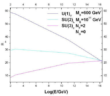
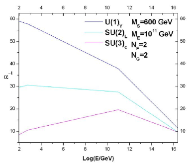
Figure 1: One-loop RGE running of the three gauge couplings. The left frame shows the case with $N_{G}=0$ while the right frame with $N_{G}=2$. In the left frame, the unification of flipped $SU(5)$ into $SO(10)$ is possible only when contributions of the profiles to the threshold corrections are taken into account.

In addition, we present the strongly coupled unification scales from our numerical calculations for $N_{G}=0$ in Table 2. These results are independent of the messenger scale $M_{E}$ and the messenger numbers $N_{F}$. In this scenario with $N_{F}$ pairs of ${\bf(5,-2)}$ and ${\bf(\bar{5},2)}$ messengers, the strongly coupled unification is possible due to the threshold contributions of the bulk matter profiles. The unification of flipped SU(5) into SO(10) is not possible with such choice of messengers in four dimensions or in orbifold models without kink mass terms.

If we adopt a nonzero $N_{G}$ and set the profile for ${\bf(10,1)}$ and ${\bf(\overline{10},-1)}$ to be ${\cal O}(1)$, we can get

$$2\pi\left(\alpha_{5}^{-1}-\alpha_{X}^{-1}\right)(M_{23}) = \frac{5}{2}(N_{G}-5)\ln\left(\frac{M_{*}}{M_{23}}\right)+5\ln(\frac{M_{*}\pi R}{2})+\frac{5}{4}\ln\lambda^{12}$$ (166)

$$-\frac{5}{8}\ln\lambda^{27}-\frac{5}{8}\ln\lambda^{15}+\frac{5}{4}\ln(Z^{1}_{n}Z^{2}_{n}{\cdots}Z^{2N_{G}}_{n})$$

$$\simeq \frac{5}{2}(N_{G}-5)\ln\left(\frac{M_{*}}{M_{23}}\right)+5\ln(\frac{M_{*}\pi R}{2})+17.034$$

with the last step obtained by taking $Z_{n}^{i}=1$. The numerical results for strongly coupled unification scale and non-zero $N_{G}$ are given in Table 3. In fact, it is more advantageous to choose the case with $N_{G}\neq 0$ not only because it can realize successful unification in four dimensions and ordinary orbifold models without kink mass terms, but also because it can satisfy the consistency requirements that the strongly coupled unification scale $M_{U}$ is much higher than $M_{C}^{*}$.

Table 2: The strongly coupled unification scale $M_{U}=M_{*}$ versus the compactification scale $M_{C}^{*}\equiv\pi R/2$ and the soft SUSY breaking mass scale $M_{S}$ for $N_{G}=0$ in the units of GeV. The symbol $``\backslash"$ marks the fact that no acceptable unification occurs.

$M_{S}[M_{23}]{\backslash}M_{C}^{*}$	$3.0\times 10^{16}$	$4.0\times 10^{16}$	$5.0\times 10^{16}$	$6.0\times 10^{16}$
$0.3\times 10^{3}[2.558\times 10^{16}]$	$1.394\times 10^{17}$	$1.151\times 10^{17}$	$9.918\times 10^{16}$	$8.783\times 10^{16}$
$0.6\times 10^{3}[2.633\times 10^{16}]$	$1.218\times 10^{17}$	$1.006\times 10^{17}$	$8.668\times 10^{16}$	$7.676\times 10^{16}$
$1.0\times 10^{3}[2.689\times 10^{16}]$	$1.103\times 10^{17}$	$9.107\times 10^{16}$	$7.848\times 10^{16}$	$6.950\times 10^{16}$
$1.5\times 10^{3}[2.735\times 10^{16}]$	$1.020\times 10^{17}$	$8.416\times 10^{16}$	$7.253\times 10^{16}$	$6.423\times 10^{16}$
$5.0\times 10^{3}[2.876\times 10^{16}]$	$8.068\times 10^{16}$	$6.660\times 10^{16}$	$5.740\times 10^{16}$	$\backslash$

Table 3: The strongly coupled unification scale $M_{U}=M_{*}$ versus the compactification scale $M_{C}^{*}\equiv\pi R/2$ and the soft SUSY breaking mass scale $M_{S}$ for $N_{G}=2$ in GeV units. The symbol $``\backslash"$ signifies the fact that no acceptable unification occurs.

$M_{S}[M_{23}]{\backslash}M_{C}^{*}$	$8.0\times 10^{16}$	$2.0\times 10^{17}$	$6.0\times 10^{17}$	$1.0\times 10^{18}$
$0.3\times 10^{3}[2.558\times 10^{16}]$	$2.946\times 10^{20}$	$4.714\times 10^{19}$	$5.238\times 10^{18}$	$1.886\times 10^{18}$
$0.6\times 10^{3}[2.633\times 10^{16}]$	$1.883\times 10^{20}$	$3.013\times 10^{19}$	$3.348\times 10^{18}$	$1.205\times 10^{18}$
$1.0\times 10^{3}[2.689\times 10^{16}]$	$1.354\times 10^{20}$	$2.166\times 10^{19}$	$2.407\times 10^{18}$	$\backslash$
$1.5\times 10^{3}[2.735\times 10^{16}]$	$1.042\times 10^{20}$	$1.667\times 10^{19}$	$1.852\times 10^{18}$	$\backslash$
$5.0\times 10^{3}[2.876\times 10^{16}]$	$4.788\times 10^{19}$	$7.661\times 10^{18}$	$8.512\times 10^{17}$	$\backslash$

7 Proton Decay

One of the unique GUT predictions is proton decay. There are several sources in SUSY GUT models: (i) The conventional lepto-quark vector gauge boson exchange which will lead to dimension six baryon number violating operators; (ii) The new contributions from supersymmetry.

The dominant new contribution in SUSY GUTs comes from the F-type dimension five baryon number violating operators

$${\cal O}_{\Delta B\neq 0}=\frac{1}{M_{U}}Q_{i}^{T}C^{-1}\tau_{2}Q_{j}\tilde{Q}_{k}^{T}\tau_{2}\tilde{L}\epsilon^{ijk}~{},$$ (167)

which can arise from triplet Higgsino exchange in the presence of a triplet Higgsino mass insertion term $M_{H}^{T}\tilde{\overline{H}}\tilde{H}$. Although this operator cannot induce proton decay at the lowest order because it is composed of squarks and sleptons, they can cause proton decay once gaugino loops are included. Thus, we anticipate a proton lifetime $\tau_{P}\sim(M_{H}^{T})^{2}$ which may not be consistent with the unification scale and then cause a problem. In the previous discussions we pointed out that the D-T splitting problem in SUSY GUTs is intimately related to the dimension five proton decay problem. In flipped SU(5), the problem of D-T splitting can be naturally solved via the elegant missing partner mechanism. In particular, the mixing term between the triplet Higgsinos is absent due to R-symmetry, thus it will not cause proton decay.

The direct $\mu$-term $\mu\bar{h}h$ is forbidden by the R-symmetry because of the following reason. From the superpotential we have

$$R(HHh)+R(\overline{H}\overline{H}\bar{h})=R(\bar{h}h)+2R(\overline{H}H)=4~{}.~{}\,$$ (168)

The superpotential terms where $H$ and $\overline{H}$ acquire VEVs indicate that $R(\bar{H}H)=0$ which means $R(\bar{h}h)=4$. It is obvious that such $\mu$-term is prohibited by R-symmetry. An effective $\mu$-term can be generated through Giudice-Masiero mechanism [51] by introducing some gauge singlets $Z$ with R-charge $4$. The effective Kahler potential is

$$K = \left(\frac{1}{\Lambda}Z^{\dagger}h\bar{h}+h.c.\right)+\frac{1}{\Lambda^{2}}Z^{\dagger}Zh^{\dagger}h+\frac{1}{\Lambda^{2}}Z^{\dagger}Z\bar{h}^{\dagger}\bar{h}+\cdots~{},~{}$$ (169)

while the $B\mu$-term $Z^{\dagger}Zh\bar{h}/\Lambda^{2}$ is forbidden in the potential. After the singlet $Z$ gets a VEV

$$\langle Z\rangle=Z_{0}+\theta^{2}Z_{F}$$ (170)

which breaks SUSY and R-symmetry, an effective $\mu$-term can be generated: $\mu\sim Z_{F}/\Lambda$. Although the $B\mu$-term is forbidden by R-symmetry, such term can arise from gaugino loops and can be naturally small compared to the $\mu$-term. The possible UV completion, which gives the interaction between the singlet $Z$ and the hidden SUSY breaking sector, is rather complicated. Thus, for simplicity we will not present a realistic model here. The small effective $\mu$-term will not reintroduce the proton decay problem since the decay process will have an additional suppression factor $(\mu/M_{H})^{2}$.

We can impose R-parity to forbid dimension-four proton decay interactions. Additional interactions leading to dangerous dimension five operators, besides those by heavy Higgsino exchange, can be introduced on the gauge symmetry breaking $O^{\prime}$ brane as follows

$$W\sim[\delta(y-\pi R/2)+\delta(y+\pi R/2)]\frac{(\psi_{2})^{2}}{M_{Pl}^{3}}\lambda^{abcd}F_{a}\bar{f}_{b}\bar{f}_{c}l^{c}_{d}~{},$$ (171)

after $\psi_{2}$ acquires a VEV. Here $a,~{}b,~{}c$, and $d$ are family indices and the R-charge of the gauge singlets is $R(\psi_{2})=1$. It corresponds to an effective dimension-five operator suppressed by $M_{pl}^{3}/M^{2}\sim 10^{30}{\rm GeV}$. Such operators will certainly not violate the current proton decay lower bound.

8 Conclusions

We proposed a realistic flipped $SU(5)$ model from an orbifolded $SO(10)$ model. The SM fermion masses and mixings were obtained via the traditional Froggatt-Nielsen mechanism and the five-dimensional wave function profiles of the SM fermions. The breaking of $N=1$ supersymmetry after orbifolding was realized via tree-level spontaneous R-symmetry breaking in the hidden sector and extra(ordinary) gauge mediation. We generated realistic SUSY breaking soft mass terms with non-vanishing gaugino masses. In addition, we studied the gauge coupling unification in detail by including the messenger fields at the intermediate scale and the KK states at the compactification scale. We found that the $SO(10)$ unified gauge coupling is very strong and the unification scale can be much higher than the compactificaiton scale. Finally, we briefly commented on proton decay.

References

• [1] H. Georgi and S. L. Glashow, Phys. Rev. Lett 32, 438 (1974); S. Dimopoulos and H. Georgi, Nucl. Phys. B193, 150 (1981).
• [2] H. Georgi, in Particles and Fields (1975); H. Fritzsch and P. Minkowski, Ann. Phys. 93, 193 (1975).
• [3] S. M. Barr, Phys. Lett. B112, 219 (1982).
• [4] J. P. Derendinger, J. E. Kim and D. V. Nanopoulos, Phys. Lett. B139, 170 (1984).
• [5] I. Antoniadis, J. R. Ellis, J. S. Hagelin and D. V. Nanopoulos, Phys. Lett. B194, 231 (1987).
• [6] C.Β S.Β Huang, T.Β Li, C.Β Liu, J.Β P.Β Shock, F.Β Wu and Y.Β L.Β Wu, JHEP 0610, 035 (2006).
• [7] Y.Β Kawamura, Prog.Β Theor.Β Phys.Β 103, 613 (2000).
• [8] Y.Β Kawamura, Prog.Β Theor.Β Phys.Β 105, 999 (2001).
• [9] Y.Β Kawamura, Prog.Β Theor.Β Phys.Β 105, 691 (2001).
• [10] G.Β Altarelli and F.Β Feruglio, Phys.Β Lett.Β B 511, 257 (2001).
• [11] L.Β J.Β Hall and Y.Β Nomura, Phys.Β Rev.Β D64, 055003 (2001).
• [12] A.Β B.Β Kobakhidze, Phys.Β Lett.Β B514, 131 (2001).
• [13] A.Β Hebecker and J.Β March-Russell, Nucl.Β Phys.Β B613, 3 (2001).
• [14] A.Β Hebecker and J.Β March-Russell, Nucl.Β Phys.Β B625, 128 (2002).
• [15] T.Β Li, Phys.Β Lett.Β B520, 377 (2001).
• [16] T.Β Li, Nucl.Β Phys.Β B619, 75 (2001).
• [17] T. Li, F. Wang and J. M. Yang, Nucl. Phys. B820, 534 (2009).
• [18] C. Balazs, T. Li, F. Wang and J. M. Yang, JHEP 0909, 015 (2009).
• [19] R. Dermisek and A. Mafi, Phys. Rev. D65, 055002 (2002).
• [20] H. D. Kim and S. Raby, JHEP 0301, 056 (2003).
• [21] S.M. Barr and I. Dorsner, Phys. Rev. D66, 065013 (2002).
• [22] I. Dorsner, Phys. Rev. D69, 056003 (2004).
• [23] C. D. Froggatt and H. B. Nielsen, Nucl. Phys. B147, 277 (1979).
• [24] K. Y. Choi J. E. Kim and H. M. Lee, JHEP 0306, 040 (2003).
• [25] Y. Nomura and M. Papucci, Phys. Lett. B661, 145 (2008).
• [26] Y. Nomura, M. Papucci and D. Stolarski, Phys. Lett. B661, 145 (2008).
• [27] A. Hebecker and J. March-Russell, Phys. Lett. B541, 338 (2002).
• [28] N. Arkani-Hamed and M. Schmaltz, Phys. Rev. D61, 033005 (2000).
• [29] N. Arkani-Hamed, L. Hall, D. Smith and N. Weiner, Phys. Rev. D63 (2001) 056003; N. Arkani-Hamed, T. Gregoire and J.Wacker, JHEP 0203 (2002) 055.
• [30] Y. Nomura, D. Smith and N. Weiner, Nucl. Phys. B613, 147 (2001).
• [31] L. Wolfenstein, Phys. Rev. Lett. 51, 1945 (1983).
• [32] A. E. Nelson and N. Seiberg, Nucl. Phys. B416, 46 (1994).
• [33] K. Intriligator, N. Seiberg and D. Shih, JHEP 0604, 021 (2006).
• [34] K. Intriligator and N. Seiberg, Class. Quant. Grav. 24, S741 (2007).
• [35] S. Ray, Phys. Lett. B642, 137 (2006).
• [36] Z. Komargodski and D. Shih, JHEP 0904, 093 (2009).
• [37] D. Shih, JHEP 0802, 091 (2008).
• [38] L. M. Carpenter, M. Dine, G. Festuccia and J. D. Mason, Phys. Rev. D79, 035002 (2009).
• [39] Z. Sun, JHEP 0901, 002 (2009).
• [40] Z. Sun, Nucl. Phys. B815, 240 (2009).
• [41] G.F. Giudice and R. Rattazzi, Nucl. Phys. B511, 25 (1998).
• [42] C. Cheung, A. L. Fitzpatrick and D. Shih, JHEP 0807, 054 (2008)
• [43] L. Randall and R. Sundrum, Nucl. Phys. B557, 79 (1999).
• [44] J. Bagger, E. Poppitz, and L. Randall, Nucl. Phys. B426, 3 (1994).
• [45] J. E. Kim and G. Carosi, arXiv:0807.3125.
• [46] C. D. Coughlan, W. Fishler, E. W. Kolb, S. Raby and G. G. Ross, Phys. Lett. B131, 59 (1983).
• [47] Y. Nomura, D. Smith, N. Weiner, Nucl. Phys. B613, 147 (2001).
• [48] K. Choi, I. W. Kim and W. Y. Song, Nucl. Phys. B687, 101 (2004).
• [49] Y. Nomura, Phys. Rev. D65, 085036 (2002).
• [50] C. Amsler et al. [Particle Data Group], Phys.Β Lett.Β B667, 1 (2008).
• [51] G. Giudice and A. Masiero, Phys. Lett. B206, 480 (1988).