Rotation of a Bose-Einstein Condensate held under a toroidal trap

Abstract

The aim of this paper is to perform a numerical and analytical study of a rotating Bose Einstein condensate placed in a harmonic plus Gaussian trap, following the experiments of bssd . The rotational frequency $\Omega$ has to stay below the trapping frequency of the harmonic potential and we find that the condensate has an annular shape containing a triangular vortex lattice. As $\Omega$ approaches $\omega$, the width of the condensate and the circulation inside the central hole get large. We are able to provide analytical estimates of the size of the condensate and the circulation both in the lowest Landau level limit and the Thomas-Fermi limit, providing an analysis that is consistent with experiment.

I. INTRODUCTION

The investigation of rotating gases or liquids is a central issue in the theory of superfluidity since they give rise to quantized vortices Lifshitz ; Donnelly91 . During recent years, several experiments using rotating atomic Bose Einstein condensates have led to the observation of vortices. These condensates are usually confined in a harmonic potential with cylindrical symmetry around the rotation axis $z$. Two limiting regimes occur depending on the ratio of the rotation frequency $\Omega$ and the trap frequency $\omega$ in the $xy$ plane. When $\Omega$ is notably smaller than $\omega$, only one or a few vortices are present at equilibrium mat ; madison . A Thomas Fermi analysis can be performed to analyze this regime because the coupling constant describing the interactions is often large in the experiments Fetter07 ; Fetter09 . When $\Omega$ approaches $\omega$, since the centrifugal force nearly balances the trapping force, the radius of the rotating gas increases, and the vortices arrange themselves on a triangular lattice Ketterle1 ; Boulder03 ; Boulder04 ; Boulder04bis . A new class of phenomena in this regime of fast rotation is predicted in relation with Quantum Hall physics Fetter09 ; C08 ; ho ; fb ; bp ; WBP ; KCR ; abd . Indeed the one-body Hamiltonian written in the rotating frame is similar to that of a charged particle in a uniform magnetic field and one can use the Landau levels structure to analyze the ground state of the condensate and describe the properties of the lattice.

In order to analyze the regime of fast rotation, one approach consists in adding a quartic potential to the harmonic potential. For this type of potential, the trapping force is always greater than the centrifugal force so that the regime $\Omega>\omega$ can be explored. The condensate is then seen to exhibit a more complex structure with regards to its density distribution and the arrangement of vortices ktu ; fjs ; Aftalion03 ; abd ; FZ ; kf ; br ; cjs . In particular, a multiply quantized vortex, or giant vortex, appears for large values of the rotational frequency $\Omega$ and the condensate is located within a thin annulus fjs . When $\Omega$ is decreased from this situation, a circle of vortices exists inside the condensate FZ .

A number of experiments have been performed in which a laser beam is shone into an otherwise harmonically trapped condensate bssd ; ss ; racnhp ; wnsbda , thus creating a trapping potential of the form harmonic plus Gaussian. Often in experiments, the laser beam is weak, hence the Gaussian term is small and for the purpose of analysis can be expanded so that the resulting potential can be approximated by a harmonic plus quartic potential. A different approach to analyze these experiments is to consider the full harmonic plus Gaussian trapping potential.

The aim of this paper is to perform a numerical and analytical study of a rotating condensate placed in a harmonic plus Gaussian trap as in the experiment bssd ; ss . The specific feature of the Gaussian potential with respect to the quartic one is that the rotation frequency $\Omega$ cannot get arbitrarily large but stays below $\omega$, the trapping frequency of the harmonic potential. We will show that according to the parameters of the system, the condensate can either be a disk or an annulus. Furthermore we will show that as $\Omega$ approaches $\omega$, the condensate always expands to become a large annulus with a vortex lattice inside the condensate and a large circulation within the central hole. This is in contrast to the harmonic plus quartic trap, which develops a giant vortex and a thin annulus. Using the Lowest Landau level (LLL) states, we will give an analytical description of the phenomena seen numerically. We estimate the radii $R_{1}$, $R_{2}$ of the condensate and the circulation around the inside hole, of order $R_{1}R_{2}$, thus much bigger than that given by a uniform lattice (which would be $R_{1}^{2}$).

This paper is organised as follows. Section II contains a brief formalisation of the problem, introducing the energy functional followed by various numerical observations in Sect. III. The lowest Landau level analysis for the regime $\Omega$ close to $\omega$ is presented in section IV which provides the main analytical results of the paper. Finally, section V is devoted to extra computations in the Thomas-Fermi regime.

II. FORMULATION

A two-dimensional Bose-Einstein condensate trapped at absolute zero temperature can be described by a macroscopic condensate wave function (order parameter) $\Psi$. The ground state of the rotating system is determined by minimizing the energy functional $E^{\prime}=E-\Omega L_{z}$ where $L_{z}=\Psi^{*}[\hat{z}\cdot(\bm{r}\times\bm{p})]\Psi$ is the $z$ component of angular momentum along the rotation axis (for linear momentum $\bm{p}$). The energy functional, in the frame rotating with angular velocity $\Omega$ is then

$$E^{\prime}=\int_{\mathcal{V}}\left[\frac{\hbar^{2}}{2m}|\nabla\Psi|^{2}+V_{tr}(r)|\Psi|^{2}+\frac{U_{0}}{2}|\Psi|^{4}-\Omega L_{z}\right]dV,$$ (1)

with $r^{2}=x^{2}+y^{2}$ and where the integral is carried out over the spatial domain $\mathcal{V}$. The trapping potential is composed of a harmonic plus Gaussian term

$$V_{tr}=V_{0}\exp{(-2r^{2}/w_{0}^{2})}+\frac{1}{2}m\omega^{2}r^{2}.$$ (2)

When the atoms are assumed to occupy the ground state of the harmonic oscillator in the $z$ direction, with energy $\hbar\omega_{z}/2$ and extension $a_{z}=\sqrt{\hbar/m\omega_{z}}$, suppression of the condensate in the $z$ direction is allowed provided the characteristic energy $\hbar\omega_{z}$ is very large in comparison with the other energy scales. Here $\omega_{z}$ is the frequency of the confinement in the $z$ direction. The two-dimensional coupling parameter is then $U_{0}=\sqrt{8\pi}\hbar^{2}a_{s}N/ma_{z}$ for $N$ identical atoms with s-wave scatting length $a_{s}$ abd .

The system can be nondimensionalised by choosing $\omega$, $\hbar\omega$ and $\sqrt{\hbar/(m\omega)}$ as units of frequency, energy and length respectively. Thus, on defining a non-dimensional coupling parameter $g=mU_{0}/\hbar^{2}$, the energy functional takes the non-dimensionalised form

$$E^{\prime}=\int_{\mathcal{V}}\left[\frac{1}{2}|\nabla\psi|^{2}+V(r)|\psi|^{2}+\frac{g}{2}|\psi|^{4}-\Omega L_{z}\right]dV,$$ (3)

for external toroidal potential trap

$$V(r)=Ae^{-l^{2}r^{2}}+\frac{1}{2}r^{2},$$ (4)

with $A=V_{0}/\hbar\omega$ and inverse waist $l=(2\hbar/m\omega w_{0}^{2})^{1/2}$. The energy functional (3) is subject to the normalization

$$\int_{\mathcal{V}}|\psi|^{2}r\,dV=1.$$ (5)

In this scaling, large rotation implies that $\Omega$ gets close to 1. Note that in experiments $l$ is often small so that the potential $V(r)$ in Eq. (4) can be expanded to give

$$V(r)\sim\frac{1}{2}(1-2Al^{2})r^{2}+\frac{1}{2}Al^{4}r^{4},$$ (6)

from which a critical frequency around $1-2Al^{2}$ is observed fjs . However in this paper we retain the toroidal potential given by Eq. (4) for the numerical and analytical analysis.

We will perform a full numerical analysis of the experimental case of bssd , which will lead us to a numerical and analytical description of several model cases which prove to be different from the harmonic plus quartic trap considered in fjs ; FZ . In particular, as $\Omega$ gets close to 1, the condensate has an annular shape, its width always becomes large and a vortex lattice is present with a circulation inside the annulus. We are able to estimate these various quantities.

III. NUMERICAL OBSERVATIONS

.1 A. The Effective Potential

When the condensate is put into rotation, the effective trapping potential to be considered is not given by Eq. (4) but is instead given by

$$V_{eff}=V(r)-\frac{1}{2}\Omega^{2}r^{2}.$$ (7)

Therefore according to the values of $A$, $l$ and $\Omega$, this effective potential can produce either a disk condensate or an annular condensate. To see this, notice first that the effective potential (7) has a minimum that occurs for $r=r_{0}\geq 0$ given by

$$r_{0}^{2}=\frac{1}{l^{2}}\log\left(\frac{2Al^{2}}{1-\Omega^{2}}\right),$$ (8)

provided

$$q\equiv\frac{2Al^{2}}{1-\Omega^{2}}\geq 1.$$ (9)

If $q\geq 1$, the effective potential has a local minimum and it can lead to two different situations, either the condensate is a disk or an annulus. For existence of an inner boundary, we must have $q\geq 1+\delta$ for some positive (not necessarily small) $\delta$. As $\Omega\rightarrow 1$, $q\geq 1+\delta$ is always satisfied and so that an inner boundary is created. The determination of the value of $\delta$ is not readily obtained as it depends on the normalisation condition (5). Conversely if $q<1$, then the condensate is always a disk.

Figure 1 shows three examples of the effective potential (7) plotted against radial distance from the centre of the condensate along constant $\theta$ for the parameters $\{g,A,l\}=\{100,25,0.03\}$, $\{1000,10,0.75\}$ and $\{500,100,0.9\}$ with $\Omega=0$. In the first parameter set $q<1$, the condensate is a disk and the density maximum is at the centre. In the second parameter set, there is a local density minimum at the centre of the condensate, but the condensate is still a disk. The third parameter set displays an inner boundary and the condensate is thus annular.

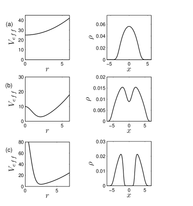
Figure 1: The effective potential given by Eq. (7) as a function of radial position is shown in the left column. The associated density ($\rho=|\psi|^{2}$) plots taken along $y=0$ are shown in the right column. Three parameter sets considered are (a) $\{g,A,l\}=\{100,25,0.03\}$, (b) $\{1000,10,0.75\}$ and (c) $\{500,100,0.9\}$ all with $\Omega=0$. Distances are measured in units of $\sqrt{\hbar/(m\omega)}$, density in units of $m\omega/\hbar$ and potentials in units of $\hbar\omega$.

The effective potential plotted in Fig. 1 only considers a non-rotating condensate, $\Omega=0$. When the condensate is placed under rotation, vortices form and the shape and size of the condensate alter. Numerical simulations on the Gross-Pitaevskii equation are carried out to explore the effect of $\Omega$ on a range of parameter sets for $\{g,A,l\}$. The two-dimensional, dimensionless, Gross-Pitaevskii equation comes directly from the energy functional (3) and is

$$i\frac{\partial\psi}{\partial t}=-\frac{1}{2}\nabla^{2}\psi+(V(r)+g|\psi|^{2})\psi-i\Omega\left(y\frac{\partial\psi}{\partial x}-x\frac{\partial\psi}{\partial y}\right),$$ (10)

for $V(r)$ given by (4). The Gross-Pitaevskii equation is solved numerically in imaginary time (see cjs ; fjs ) by evolving an initial wavefunction for a range of values of $\Omega<1$ in order to find the ground state. Three cases of interest, which summarise the numerical results well, are presented below. The three reported parameter sets are; $\{g,A,l\}=\{955.95,24.83,0.07\}$, $\{14,1000,5\}$ and $\{500,60,0.1\}$.

.2 B. The Experimental Case of Bretin et al. bssd

A natural case to numerically simulate is that considered experimentally by Bretin et al. bssd where a harmonically trapped condensate is put in rotation with a weak laser beam shone at the origin, modeled by a Gaussian term. This experimental case can be described by a two dimensional system as explained in the introduction, using the dimensional reduction which leads to the definition of $U_{0}$. The experimental values of bssd correspond to $\{g,A,l\}=\{955.95,24.83,0.07\}$. A series of contour plots of the density are shown in Fig. 2 (see Fig. 1 of bssd , with the appropriate rescaling of rotational velocities, so that the $\Omega_{\text{stir}}^{(2)}=60$ of bssd corresponds to $\Omega=0.795$ in this paper and $\Omega_{\text{stir}}^{(2)}=69$ corresponds to $\Omega=0.914$. The rotational velocity is calculated from bssd using the value of the frequency in the $x$ and $y$ direction $\omega_{\perp}^{(0)}/2\pi=75.5Hz$ and not the second stirring phase frequency $\omega_{\perp}/2\pi=64.8Hz$).

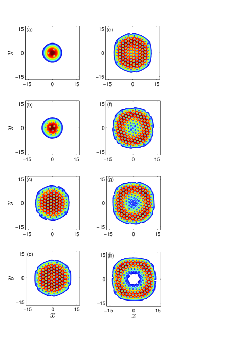
Figure 2: (Color online) Density profiles of a rotating condensate with $\{g,A,l\}=\{955.95,24.83,0.07\}$ corresponding to the (non-dimensionalised) experimental values of bssd for (a) $\Omega=0.25$, (b) $\Omega=0.5$, (c) $\Omega=0.874$, (d) $\Omega=0.887$, (e) $\Omega=0.901$, (f) $\Omega=0.914$, (g) $\Omega=0.92$ and (h) $\Omega=0.93$. Distances are measured in units of $\sqrt{\hbar/(m\omega)}$.

For the slow rotational velocities ($\Omega\lesssim 0.5$) of Fig. 2, the condensate is a disk with a small number of vortices (12 vortices are present when $\Omega=0.5$; see Fig. 2(b)) with the vortices forming a triangular lattice. As the rotational velocity is increased, the radius of the outer boundary increases while more vortices are accommodated into the condensate. The dynamics here mimic those observed in harmonic traps.

Above some angular velocity the density at the centre of the condensate begins to deplete and eventually an inner boundary, hence an annulus, is created. In the experiments of bssd , a density minimum at the centre first occurred for $\Omega\sim 0.874$ (corresponding to $\Omega_{\text{stir}}^{(2)}=66$; see plate (c) of Fig. 1 in bssd ). The numerical simulations here suggest the onset of the density minimum to be $\Omega\sim 0.887$; see plate (d) of Fig. 2 where the density minimum first appears. Clearer pictures of the development of the depletion of density at the centre can be seen in plates (e) and (f). It distorts the vortex lattice in much the same way that the outer boundary does. In Sect IV we note that, under the LLL approximation, the vortex lattice inside the central hole is distorted from a regular vortex lattice such that the number of zeros in the hole is given by $R_{1}R_{2}$, to get a number of order $R_{1}^{2}$, where $R_{1},R_{2}$ are the inner, outer radii. Increasing the angular velocity still further, thus exploring the fast rotation regime $\Omega\rightarrow 1$, details how the density at the centre of the condensate continues to diminish until for $\Omega\sim 0.92$ a central hole develops (see plate (g)) and the condensate becomes annular. The central hole grows rapidly; for $\Omega=0.93$, the central hole is large and there is a circulation equivalent to $11$ vortices (see plate (h)). Our simulations have been carried out up to $\Omega\sim 0.95$. These higher angular velocity simulations suggest that both the outer and inner radii and also the width of the condensate increase in size as $\Omega\rightarrow 1$.

The experiments of Bretin et al. bssd provide an example of the transition from a disk condensate with the density maximum at the center to a disk condensate with a local minimum at the center. It is reasonably safe to assume that if the angular velocity could be further increased in the experiments, the condensate would become annular, with a large persistent current. The depletion of density, which occurs for $\Omega\gtrsim 0.887$, creating a distortion in the vortex lattice and requiring a longer time of convergence for the numerical simulations, must be one of the reasons that explain the experimental difficulties in observing the condensate at these rotation frequencies.

.3 C. The Annulus

Manipulating the values of the parameters $\{g,A,l\}$ can have the effect of altering the shape of the condensate. Here we will consider a parameter set that creates an annular condensate that is present for all $\Omega<1$. The parameter set is thus chosen to be $\{g,A,l\}=\{14,1000,5\}$. A selection of contour plots for various angular velocities are given in Fig. 3. The choice of this parameter set is to illustrate the behaviour as $\Omega$ gets close to 1.

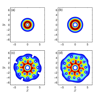
Figure 3: (Color online) Density profiles of a rotating condensate with $\{g,A,l\}=\{14,1000,5\}$ for (a) $\Omega=0.25$, (b) $\Omega=0.9$, (c) $\Omega=0.99$ and (d) $\Omega=0.994$. Distances are measured in units of $\sqrt{\hbar/(m\omega)}$.

For low rotational velocities, see Fig. 3(a), the condensate does not contain vortices in the annulus. However the closer $\Omega$ approaches unity, both the radius of the inner and outer boundaries increase, but so too does the width of the condensate. When $\Omega=0.9$ (Fig. 3(b)), the condensate still does not contain any vortices, but for $\Omega=0.99$ (Fig. 3(c)), the condensate contains two complete rings of vortices. For $\Omega=0.99$, there is a multiply quantised vortex at the centre of the condensate providing a persistent flow with a quantum of circulation $\nu=3$. The phase profiles also show that there are further singularities of phase (‘invisible’ vortices) in the outer regions of the condensate.

Note that, for all $\Omega$, the condensate is always an annulus with the inner and outer radii both increasing as $\Omega$ increases. Furthermore the width of the condensate also increases so that a thin annulus is never created. The increase in size of the condensate for $\Omega>0.9$ is marked. This parameter set explicitly shows the presence, at large $\Omega$, of a central hole containing circulation together with a vortex lattice in the bulk of the condensate.

The choice of this parameter set, especially the value of $g$, is specifically chosen with reference to the lowest Landau level (LLL) analysis in Sect. IV. As will noted in Sect. IV, to use the LLL approximation requires $g(1-\Omega^{2})$ to be small. As a consequence, with an eye on the capability of the numerical simulations to resolve at $\Omega$ close to 1, it necessarily forces $g$ to be not too large, though the main features are preserved while increasing $g$. We note here that an annular condensate, existing at all $\Omega$, can be created for a wide range of values of $g$.

.4 D. Density Dip at the Center

As a final numerical example, one can consider the parameter set $\{g,A,l\}=\{500,60,0.1\}$. The choice of these parameters actually forces, for $\Omega=0$, the ground state to have a local non-zero minimum of density at the centre. For these parameters the density maximum is located at $r=4.2$ when $\Omega=0$ and the condensate is a disk; a contour plot of the condensate at $\Omega=0$ is given in Fig. 4 along with a selection of other plots for various angular velocities.

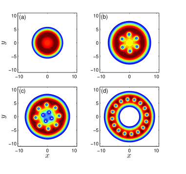
Figure 4: (Color online) Density profiles of a slow rotating condensate with $\{g,A,l\}=\{500,60,0.1\}$ and (a) $\Omega=0$, (b) $\Omega=0.225$, (c) $\Omega=0.35$ and (d) $\Omega=0.5$. Distances are measured in units of $\sqrt{\hbar/(m\omega)}$.

Vortices first appear close to the maximum of density instead of close to the center of the condensate. As $\Omega$ is increased, the vortex lattice develops close to this initial circle of vortices. The increase in size of the condensate is visible, as is the depletion of density at the centre of the condensate, which turns into a hole: an annulus is formed.

IV. Lowest Landau Level Analysis

We turn to the analysis of the ground state of the energy (3), where $V(r)$ is given by Eq. (4) and $\Omega$ tends to 1. We will use a Lowest Landau level analysis ho ; abd ; ABN2 . Recall that the spectrum of the Hamiltonian

$$H_{\Omega}=-\frac{1}{2}\nabla^{2}+\frac{1}{2}r^{2}-\Omega L_{z},$$ (11)

has a Landau level structure. The lowest Landau level is defined as

$$f(x+iy)e^{-\frac{\Omega}{2}\left(x^{2}+y^{2}\right)},\ f\text{ analytic}.$$ (12)

For such functions, $<H_{\Omega}\psi,\psi>$ can be simplified (see abd ) so that $E^{\prime}=\Omega+E_{LLL}(\psi)$ where

$$E_{LLL}(\psi)=\int_{\mathcal{V}}\left(V(r)-\frac{1}{2}\Omega^{2}r^{2}\right)|\psi|^{2}+\frac{g}{2}|\psi|^{4}dV.$$ (13)

The minimization of Eq. (13) without the analytic constraint provides the Thomas-Fermi profile for the coarse grain density:

$$|\psi|^{2}=\rho_{\rm TF}:=\lambda-\frac{1}{g}\left(V(r)-\frac{1}{2}\Omega^{2}r^{2}\right).$$ (14)

Such a function can be recovered in the LLL by the presence of the vortex lattice and this only changes the coefficient $g$ into $bg$ where $b$ is the Abrikosov parameter as we explain further below.

We recall that the orthogonal projection for a general function $\psi$ onto the LLL is explicit B ; GiJa and given by:

$$\Pi_{LLL}(\psi)=\frac{1}{\pi}\int e^{{-\frac{1}{2}\left(|z|^{2}-2z\overline{z^{\prime}}+|z^{\prime}|^{2}\right)}}\psi(x^{\prime},y^{\prime})dx^{\prime}dy^{\prime},$$ (15)

where $z=x+iy$ and $z^{\prime}=x^{\prime}+iy^{\prime}$. If an LLL function $\psi$ (i.e $\psi$ satisfies Eq. (12)) minimizes the energy Eq. (13), it is a solution of the projected Gross-Pitaevskii equation:

$$\Pi_{LLL}\left[\left({V(r)-\Omega^{2}r^{2}/2}+g|\psi|^{2}-\mu\right)\psi\right]=0,$$ (16)

where $\mu$ is the chemical potential.

When $\Omega$ is close to 1, and $V(r)$ is the harmonic plus Gaussian potential, Eq. (16) can be approximated by $\Pi_{LLL}\left[g|\psi|^{2}\psi\right]=\mu\psi,$ which is the equation of the Abrikosov problem (see ho ; ABN2 ; Abr ). A solution can then be constructed using the Theta function (see ABN2 for the details):

$$\phi(x,y;\tau)=e^{\frac{1}{2}\left({z^{2}}-{|z|^{2}}\right)}\Theta\left(\sqrt{\frac{\tau_{I}}{\pi}}z,\tau\right),$$ (17)

where $\tau=\tau_{R}+i\tau_{I}$ is the lattice parameter. The zeroes of the function $\phi$ lie on the lattice $\sqrt{\frac{\pi}{\tau_{I}}}\left(\mathbb{Z}\oplus\mathbb{Z}\tau\right)$ and $|\phi|$ is periodic. The optimal lattice, that is the one minimizing $\mu(\tau)=\int|\phi|^{4}/(\int|\phi|^{2})^{2}$, is hexagonal, which corresponds to $\tau=e^{2i\pi/3}$ (the integrals are taken on one period). For $\tau=e^{2i\pi/3}$, $\mu(\tau)=b\sim 1.16$.

As in ABN2 , we can construct an approximate ground state by multiplying the solution, Eq. (17), of the Abrikosov problem by a profile $\rho$ varying on the same scale as $\rho_{\rm TF}$, which is large. Since this product is not in the LLL, we project it onto the LLL and define $v=\Pi_{LLL}\left(\sqrt{\rho(x,y)}\phi(x,y;e^{2i\pi/3})\right).$ Estimating the energy of $v$ yields

$$E_{\rm LLL}(v)\sim\int_{\mathbb{R}^{2}}\left(V(r)-\frac{1}{2}\Omega^{2}r^{2}\right)\rho(x,y)+\frac{gb}{2}\rho(x,y)^{2}.$$

This computation assumes that $\phi$ and $\rho$ do not vary on the same scale, hence the integrals can be decoupled. Then, minimizing with respect to $\rho$ implies that $\rho$ must be a Thomas-Fermi profile (Eq. (14)) with $g$ changed into $bg$:

$$\rho(x,y)=\lambda-\frac{1}{bg}\left(V(r)-\frac{1}{2}\Omega^{2}r^{2}\right).$$ (18)

This approximation is valid provided the energy obtained, $E_{\rm LLL}(v)$, is much smaller than the gap between two Landau levels which is of the order unity.

In the case of the harmonic potential $V(r)=r^{2}/2$, the Thomas Fermi profile provides a disk condensate of radius $R=[4gb/(\pi(1-\Omega^{2}))]^{1/4}$ which is large when $\Omega$ gets close to 1. Moreover, $E_{\rm LLL}(v)$ is of order $\sqrt{g(1-\Omega^{2})}$ which is indeed small when $\Omega$ is close to 1 and $g$ is not too large, so that the LLL approximation is satisfied. In the case of the toroidal potential (4), we have to compute the Thomas-Fermi profile from Eq. (18) and discriminate whether it is a disk or an annulus. Then we have to check whether the LLL approximation is justified, that is whether $E_{LLL}(v)$ is small.

A. Disc Condensate

Suppose that the condensate is a disk (recall that this requires that $q$ is not too large), so that only an outer boundary exists and write

$$gb|\psi|^{2}=\mu+\frac{1}{2}(\Omega^{2}-1)r^{2}-Ae^{-l^{2}r^{2}}.$$ (19)

To find approximations to the radius of the outer boundary one can proceed by taking Eq. (19) and the normalization condition (5) which provide the necessary starting equations in order to compute $\mu$. A check on the validity of the LLL approximation is to verify, in the limit $\Omega\rightarrow 1$, that the chemical potential $\mu$ is small.

To begin, substitute the density, $|\psi|^{2}$, from Eq. (19) into the normalization condition (5) and integrate over the domain between $0$ and $R_{2}$, where $R_{2}$ is defined as the radius of the outer boundary. It follows that

$$\frac{gb}{\pi}=\mu R_{2}^{2}+\frac{1}{4}(\Omega^{2}-1)R_{2}^{4}+\frac{A}{l^{2}}(e^{-l^{2}R_{2}^{2}}-1),$$ (20)

which explicitly contains the chemical potential $\mu$. To remove $\mu$ from the calculations, one can note from Eq. (19) that

$$\frac{\mu-V_{eff}(r)}{gb}\bigg{|}_{R_{2}}=|\psi|^{2}\big{|}_{R_{2}}=0,$$ (21)

from which

$$\mu=Ae^{-l^{2}R_{2}^{2}}-\frac{1}{2}(\Omega^{2}-1)R_{2}^{2}.$$ (22)

Using Eq. (22) in Eq. (20) gives

$$\frac{gb}{\pi}=\frac{1}{4}(1-\Omega^{2})R_{2}^{4}+A\left[R_{2}^{2}e^{-l^{2}R_{2}^{2}}+\frac{1}{l^{2}}(e^{-l^{2}R_{2}^{2}}-1)\right].$$ (23)

At this stage we introduce the parameter $p$, defined as

$$p\equiv\frac{gl^{4}}{\pi(1-\Omega^{2})}.$$ (24)

We are interested in the limit $\Omega$ close to 1, i.e. $p\gg 1$, which corresponds to $l^{2}R_{2}^{2}\gg 1$. Then the exponential terms in Eq. (23) immediately disappear and it follows that

$$R_{2}\sim\left(\frac{4}{(1-\Omega^{2})}\left[\frac{gb}{\pi}+\frac{A}{l^{2}}\right]\right)^{1/4}$$ (25)

and

$$\mu\sim\left((1-\Omega^{2})\left[\frac{gb}{\pi}+\frac{A}{l^{2}}\right]\right)^{1/2}.\\$$ (26)

This implies that $l^{2}R_{2}^{2}$ is large and $\mu$ is small since $\Omega$ is close to 1. Recall that the assumption of a disk condensate requires $q$ to be bounded, $q<1+\delta$, and thus (as $\delta$ is not large)

$$Al^{2}<\frac{(1+\delta)(1-\Omega^{2})}{2},$$ (27)

so that the ratio $Al^{2}$ has to be small in this regime.

B. Annular Condensate

Expressions (25)-(26) are valid strictly when there is no inner boundary which occurs when $q<1+\delta$. If $q\geq 1+\delta$ then an inner boundary, at $r=R_{1}$, develops.

One again starts from Eq. (19), but this time the integration is taken over the domain between $R_{1}$ and $R_{2}$. It then follows that

$$\frac{gb}{\pi}=\mu(R_{2}^{2}-R_{1}^{2})+\frac{1}{4}(\Omega^{2}-1)(R_{2}^{4}-R_{1}^{4})+\frac{A}{l^{2}}\left(e^{-l^{2}R_{2}^{2}}-e^{-l^{2}R_{1}^{2}}\right),$$ (28)

which again explicitly contains the chemical potential $\mu$. To remove $\mu$ from the calculations, we note from Eq. (19) that

$$\frac{\mu-V_{eff}(r)}{gb}\bigg{|}_{R_{1},R_{2}}=|\psi|^{2}\big{|}_{R_{1},R_{2}}=0,$$ (29)

from which we recover Eq. (22) and

$$e^{-l^{2}R_{2}^{2}}-e^{-l^{2}R_{1}^{2}}=\frac{1}{2A}(\Omega^{2}-1)(R_{2}^{2}-R_{1}^{2}).$$ (30)

Upon substitution of Eq. (22) and Eq. (30) into Eq. (28) and writing the ‘area’ of the annulus as $X\equiv R_{2}^{2}-R_{1}^{2}$, we get

$$gb=\frac{1}{2}\pi X(\Omega^{2}-1)\left[\frac{Xe^{-l^{2}X}}{e^{-l^{2}X}-1}+\frac{1}{l^{2}}-\frac{X}{2}\right].$$ (31)

Since $p$ is large (because $\Omega$ is close to 1), we can assume that $l^{2}X$ is large so that the first term in the squared brackets of Eq. (31) is negligible, which leaves

$$gb=\frac{1}{2}\pi X^{2}(\Omega^{2}-1)\left[\frac{1}{l^{2}X}-\frac{1}{2}\right].$$ (32)

Now, as $l^{2}X$ is taken to be large, one can neglect $1/l^{2}X$ in front of the factor of a half in the square bracket. Formally, this corresponds to the following being satisfied

$$\frac{1}{1-\Omega^{2}}\gg\frac{\pi}{gl^{4}}.$$ (33)

Thus one obtains an expression for $X$,

$$X\sim\sqrt{\frac{4gb}{\pi(1-\Omega^{2})}},$$ (34)

so that $l^{2}X$ is indeed large when $\Omega$ gets close to 1. Furthermore, from (30)

$$e^{-l^{2}R_{1}^{2}}=\frac{(\Omega^{2}-1)X}{2A(e^{-l^{2}X}-1)},$$ (35)

which, on using the derived approximation for $X$, Eq. (34), implies that

$$R_{1}\sim\frac{1}{l}\left[\ln\left(A\sqrt{\frac{\pi}{gb(1-\Omega^{2})}}\right)\right]^{1/2},$$ (36)

giving an expression for the radius of the inner boundary. The value of the chemical potential can then easily be found by taking Eq. (29) evaluated at $R_{1}$, with the expression for $R_{1}$ following directly from Eq. (36);

$$\mu = \frac{1}{2}(1-\Omega^{2})R_{1}^{2}+Ae^{-l^{2}R_{1}^{2}}$$ (37)

$$\sim \sqrt{\frac{gb(1-\Omega^{2})}{\pi}},$$

provided

$$\ln\left(A\sqrt{\frac{\pi}{gb(1-\Omega^{2})}}\right)\ll\left(\frac{4gbl^{4}}{\pi(1-\Omega^{2})}\right)^{1/4}.$$ (38)

In the limit $\Omega\rightarrow 1$, we see indeed that $\mu\rightarrow 0$, thus justifying the LLL approximation provided $g$ is not too large. The radius of the outer boundary can be found by taking Eq. (22) with $\mu$ given by (37). Then

$$R_{2}\sim\left(\frac{4gb}{\pi(1-\Omega^{2})}\right)^{1/4},$$ (39)

which is just $\sqrt{X}$, implicitly implying through $(\ref{appx1})$ that $R_{2}^{2}\gg R_{1}^{2}$.

To find the width of the condensate, $d=R_{2}-R_{1}$, it is necessary that $R_{1}$ be neglected in front of $R_{2}$, i.e. that $R_{1}/R_{2}\ll 1$ which again is equivalent to Eq. (38) being satisfied. Thus, the width of the condensate $d$ is found from

$$X = (R_{2}-R_{1})(R_{1}+R_{2})$$

$$\Rightarrow d = \frac{X}{R_{1}+R_{2}}\sim\frac{X}{R_{2}}=\left(\frac{2gb}{\pi(1-\Omega^{2})}\right)^{1/4}.$$ (40)

Notice that both the width of the condensate $d$ and the inner $R_{1}$ and outer boundaries $R_{2}$ get larger as $\Omega$ increases and eventually tend to infinity as $\Omega\rightarrow 1$. However, while the width of the condensate and the outer boundary grow like $(1-\Omega^{2})^{-1/4}$, the inner boundary grows like $\ln[(1-\Omega^{2})^{-1/2}]^{1/2}$. Thus, in the limit $\Omega\rightarrow 1$, the condensate forms an infinitely thick annulus with both the inner and outer boundary tending to infinity and with an infinitely large central hole.

The Cauchy formula allows us to compute the number of zeroes $\nu(R_{1})$ inside the disk of radius $R_{1}$:

$$\nu(R_{1})=\frac{R_{1}R_{2}}{2\pi}\int_{0}^{2\pi}\!\!\!\!d\theta\frac{\int e^{\frac{R_{1}}{R_{2}}\overline{z^{\prime}}}e^{-|z^{\prime}|^{2}}\overline{z^{\prime}}\sqrt{\rho(z^{\prime})}\phi(z^{\prime}e^{-i\theta},\tau)dz^{\prime}}{\int e^{\frac{R_{1}}{R_{2}}\overline{z^{\prime}}}e^{-|z^{\prime}|^{2}}\sqrt{\rho(z^{\prime})}\phi(z^{\prime}e^{-i\theta},\tau)dz^{\prime}},$$ (41)

where $\phi$ comes from (17). Using a Laplace method to evaluate the integrals, we see that for large $R_{1}$, since $R_{1}/R_{2}$ tends to 0,

$$\nu(R_{1})\sim R_{1}R_{2}.$$ (42)

Note that a regular lattice in a disk of radius $R_{1}$ would give $\nu(R_{1})\sim R_{1}^{2}$, which is much smaller.

C. Summary of the main results

We have derived that as $\Omega$ approaches 1, the condensate has an annular shape with a triangular vortex lattice inside. Eq.’s (36), (39), (37) and (42) provide the inner, outer radii of the condensate, the chemical potential and the circulation in the inside hole. In the LLL approximation, we must have $\sqrt{g(1-\Omega^{2})}\ll 1$. Therefore in the limit $\Omega\rightarrow 1$, the parameter set $\{g,A,l\}=\{14,1000,5\}$, described in Set. IIIC and with a series of contour plots (Fig. 3) showing that the condensate is always annular, satisfies this condition. Table 1 gives a comparison between the numerical and analytical values for this parameter set and provide a good check on the estimates derived in Eq.’s (36), (37), (39) and (42).

Table 1: A comparison, for parameters $\{g,A,l\}=\{14,1000,5\}$, of the values of the inner radius $R_{1}$, outer radius $R_{2}$ and quantum of circulation $\nu$ for fast rotation calculated in the LLL and given by Eq.’s (36), (39) and (42) respectively. Numerical values are provided (subscripts $n$) as a comparison. The chemical potential $\mu$ is also given, calculated from Eq. (37).

$\Omega$	$R_{1}$	$R_{1n}$	$R_{2}$	$R_{2n}$	$\nu$	$\nu_{n}$	$\mu$
0.9	0.53	0.66	3.23	3.25	1.70	2	0.99
0.99	0.57	0.69	5.68	5.71	3.22	3	0.32
0.994	0.58	0.70	6.45	6.38	3.72	3	0.25

V. Thomas-Fermi approximation

In the case of the experiments of Bretin et al. bssd , $\Omega$ is not very close to 1 and $g$ is large, so the LLL analysis of Sect IV does not adequately describe this experiment. In order to describe it better, and since $g$ is large, we can use the Thomas-Fermi (TF) approximation. In the TF approximation, the vortex cores are a small perturbation with respect to the density profile and yield similar equations to those previously derived in Sect IV, except that now there is no factor $b$ entering the TF density profile of Eq. (19) since the vortex cores are small. These computations are similar to those in fjs , however due to the Gaussian trapping potential used here, the condensate becomes a thick annulus, with many vortices, instead of a thin annulus with no vortex as in fjs . This changes significantly the approximations and requires the analysis of several cases according to the magnitude of $l^{2}R^{2}$, $R$ being the radius of the condensate.

A. Disk condensate

If there is no inner boundary then the Thomas-Fermi approximation leads to

$$g|\psi|^{2}=\mu+\frac{1}{2}(\Omega^{2}-1)r^{2}-Ae^{-l^{2}r^{2}}.$$ (43)

We substitute the density $|\psi|^{2}$ from Eq. (43) into the normalization condition (5) and integrate over the domain between $0$ and $R_{2}$, where as before $R_{2}$ is defined as the radius of the outer boundary. It follows that

$$\frac{g}{\pi}=\mu R_{2}^{2}+\frac{1}{4}(\Omega^{2}-1)R_{2}^{4}+\frac{A}{l^{2}}(e^{-l^{2}R_{2}^{2}}-1),$$ (44)

which explicitly contains the chemical potential $\mu$. To remove $\mu$ from the calculations, one can note from Eq. (43) that

$$\frac{\mu-V_{eff}(r)}{g}\bigg{|}_{R_{2}}=|\psi|^{2}\big{|}_{R_{2}}=0,$$ (45)

from which we get

$$\mu=Ae^{-l^{2}R_{2}^{2}}-\frac{1}{2}(\Omega^{2}-1)R_{2}^{2},$$ (46)

which is the same as (22). Using Eq. (46) in Eq. (44) yields

$$\frac{g}{\pi}=\frac{1}{4}(1-\Omega^{2})R_{2}^{4}+A\left[R_{2}^{2}e^{-l^{2}R_{2}^{2}}+\frac{1}{l^{2}}(e^{-l^{2}R_{2}^{2}}-1)\right].$$ (47)

If $l$ is taken to be small as in the experiments, we can assume that $p$ is small and thus that $l^{2}R_{2}^{2}$ is small. Then the exponentials in $l^{2}R_{2}^{2}$ can be expanded and it readily follows that

$$p\sim\frac{1}{4}l^{4}R_{2}^{4}(1-q)+\frac{1}{6}ql^{6}R_{2}^{6},$$ (48)

where we have used the expressions for $q$ and $p$ (Eq.’s (9) and (24) respectively). Equation (48) is a cubic equation in $l^{2}R_{2}^{2}$. When $q<1$, the last term in Eq. (48) can be neglected and we get

$$R_{2}^{4}\sim\frac{4p}{l^{4}(1-q)}=\frac{4g}{\pi((1-\Omega^{2})-Al^{2})}.$$ (49)

When $q$ becomes larger than 1, then $1-q<0$, but since we assume that we have a disk condensate, we recall that $1-q$ is small. In such situations, the last term in Eq. (48) cannot be neglected and is crucial to get the correct sign on the right hand side of (48).

The chemical potential is derived from Eq. (46)

$$\mu\sim A\left(1-\frac{p}{q}\right)+\frac{1}{2}R_{2}^{2}(1-\Omega^{2})(1-q)+\frac{1}{4q}Al^{4}R_{2}^{4}(1+q),$$ (50)

with the value of $R_{2}$ obtained from Eq. (48). This allows us to check that $g|\psi(0)|^{2}\sim\mu-A$ is large, provided $1-\Omega^{2}$ is not too small, $g$ is large, $l$ is small so that $p$ is small. Hence, this justifies our use here of the TF approximation. This is in particular the case for the parameters $\{g,A,l\}=\{955.95,24.83,0.07\}$ corresponding to the experiments of bssd .

Table 2: A comparison, for parameters $\{g,A,l\}=\{955.95,24.83,0.07\}$, for $\Omega$ such that the condensate is a disk. The value of the radius of the condensate for different rotational velocities calculated asymptotically from Eq. (48) under the assumption of the TF approximation and calculated numerically is shown.

$\Omega$	$R_{2}$ (asymptotically)	$R_{2}$ (numerically)
0.1	6.29	6.18
0.25	6.40	6.19
0.5	6.87	6.70
0.795	8.97	9.00
0.821	9.44	9.49

Table 2 gives a comparison between the numerical values and analytical values (calculated from Eq. (48)) for the boundary of the condensate when the condensate is still a disk ($\Omega\lesssim 0.92$), with the agreement found to be extremely good.

A specific feature of our numerics in the case $\{g,A,l\}=\{500,60,0.1\}$ is to find that for certain values of the parameters, since the maximum of the density is not at the origin, that vortices appear on a specific circle rather than at the origin (see Figure 4(b)). We call $\rho(r)$ the average of $|\psi|^{2}$ on a circle of radius $r$. Then $\rho$ is not far from the TF approximation of $|\psi|^{2}$ given by (43), but not exactly since the presence of the circle of vortices has an influence on its shape. A computation similar to that in FZ would be required to determine $\rho$ in this setting. Once this is done, one should be able to use the results of A , chapter 3, which states that the radius where the circle of vortices appear is given by the location where the function $\zeta/\rho$ reaches its maximum, where $\zeta(r)=\int_{r}^{R}s\rho(s)\ ds$, $R$ being the radius of the condensate. This follows from an expansion of the Gross Pitaevskii energy, where the leading order is given by the energy of vortices of order $\rho(r)\ln\xi$, where $\xi$ is the scattering length, minus the $L_{z}$ term, which can be estimated as $-\Omega\zeta(r)$. Thus, the lowest $\Omega$ for nucleation of vortices is achieved when there is a radius where $\zeta/\rho$ is minimal.

B. Annular condensate

When the condensate is an annulus, then in the TF approximation, we need to take into account the quantum of circulation $\nu$ in the inner hole of the condensate. We assume that $\psi=|\psi|e^{i\nu S}$, where $S$ is the phase. Note that this is not needed in the LLL approach, because the circulation is incorporated into the LLL wave function and we can compute it directly from (41).

The TF density expression (43) is adjusted to

$$g|\psi|^{2}=\tilde{\mu}+\frac{1}{2}\left[(\Omega^{2}-1)r^{2}-\frac{\nu^{2}}{r^{2}}\right]-Ae^{-l^{2}r^{2}},$$ (51)

where $\tilde{\mu}=\mu+\Omega\nu$. The TF density (51) and the normalisation condition (5) provide the starting points from which approximations to the values of the radii of the condensate boundaries and thus the width of the condensate can be found. It follows then that

$$0=\tilde{\mu}+\frac{1}{2}\left[(\Omega^{2}-1)r^{2}-\frac{\nu^{2}}{r^{2}}\right]-Ae^{-l^{2}r^{2}}\bigg{|}_{R_{1},R_{2}},$$ (52)

and eliminating $\tilde{\mu}$ from Eq. (52) gives

$$\nu^{2}=R_{1}^{2}R_{2}^{2}\left[(1-\Omega^{2})+\frac{2A}{X}e^{-l^{2}R_{1}^{2}}(e^{-l^{2}X}-1)\right],$$ (53)

where $X$ is the ‘area’ of the condensate and is again defined as $X\equiv R_{2}^{2}-R_{1}^{2}$. From integration of the normalisation condition (5) between $R_{1}$ and $R_{2}$ it ensues that

$$\frac{g}{\pi} = \frac{1}{4}(1-\Omega^{2})X(R_{1}^{2}+R_{2}^{2})-\frac{1}{2}(1-\Omega^{2})R_{1}^{2}R_{2}^{2}\ln\left(\frac{R_{2}^{2}}{R_{1}^{2}}\right)$$

$$+ Ae^{-l^{2}R_{1}^{2}}(e^{-l^{2}X}-1)\left[R_{1}^{2}+\frac{1}{l^{2}}-\frac{R_{1}^{2}R_{2}^{2}}{X}\ln\left(\frac{R_{2}^{2}}{R_{1}^{2}}\right)\right]$$

$$+ AXe^{-l^{2}X}e^{-l^{2}R_{1}^{2}}.$$

A further expression that connects the quantum of circulation and the inner and outer radii is readily obtained from the minimisation of the free energy per particle, $F=E^{\prime}-\mu\bar{N}$, where $\bar{N}$ is the number of bosons in the condensate fjs . The following integral identity results:

$$g\Omega=2\nu\pi\int_{R_{1}}^{R_{2}}\frac{1}{r}\left[g|\psi|^{2}\right]dr.$$ (55)

Integration of Eq. (55) using Eq. (43), together with the expressions for $\tilde{\mu}$ and $\nu$ above, results in

$$\begin{split}\frac{g\Omega}{\pi\nu}&=\biggl{[}\frac{1}{2}(1-\Omega^{2})(R_{1}^{2}+R_{2}^{2})+Ae^{-l^{2}R_{2}^{2}}\\ &+\frac{AR_{1}^{2}}{X}e^{-l^{2}R_{1}^{2}}(e^{-l^{2}X}-1)\biggl{]}\ln\left(\frac{R_{2}^{2}}{R_{1}^{2}}\right)-X(1-\Omega^{2})\\ &-Ae^{-l^{2}R_{1}^{2}}(e^{-l^{2}X}-1)+2A\int^{R_{2}}_{R_{1}}\frac{1}{r}e^{-l^{2}r^{2}}dr.\end{split}$$ (56)

In order to proceed it becomes important to estimate the last integral in Eq. (56) according to the size of $l^{2}r^{2}$. The following sections detail two possible limits.

$l^{2}R_{2}^{2}$ small. If $l^{2}R_{2}^{2}$ is assumed to be small, then it follows that $l^{2}R_{1}^{2}$ is small as well. Thus expanding the exponential terms in Eq. (53) up to terms of order $l^{6}R_{2}^{6}$ gives

$$\nu^{2}\sim R_{1}^{2}R_{2}^{2}\left[(1-\Omega^{2})(1-q)+Al^{4}R_{2}^{2}\right],$$ (57)

where we have assumed that $R_{2}^{2}\gg R_{1}^{2}$, which implies that we can write $\exp(-l^{2}X)\sim\exp(-l^{2}R_{2}^{2})$. In the case of an annular condensate, we have that $q>1$, so that the first term in Eq. (57) is negative. Therefore in order for the right hand side of Eq. (57) to be positive, it is required that

$$l^{2}R_{2}^{2}>\frac{(q-1)(1-\Omega^{2})}{Al^{2}}=2\left(1-\frac{1}{q}\right).$$ (58)

Expansion of Eq. (LABEL:nu1) to order $l^{6}R_{2}^{6}$ (again assuming that $R_{2}^{2}\gg R_{1}^{2}$) results in an expression for $R_{2}$,

$$\begin{split}p&\sim\frac{1}{4}(1-q)l^{4}R_{2}^{2}\biggl{[}R_{2}^{2}\biggl{(}1+\frac{ql^{2}}{(1-q)}\biggl{(}\frac{R_{2}^{2}}{3}-R_{1}^{2}\ln(R_{2}^{2})\biggr{)}\biggr{)}\\ &\qquad\qquad\qquad\qquad-2R_{1}^{2}\ln(R_{2}^{2})\biggr{]}\\ &\sim\frac{l^{4}R_{2}^{4}(1-q)}{4}+\frac{ql^{6}R_{2}^{6}}{6},\end{split}$$ (59)

where we assume that $R_{2}^{2}\gg R_{1}^{2}\ln(R_{2}^{2}/R_{1}^{2})\sim R_{1}^{2}\ln(R_{2}^{2})$. Notice that (59) is actually the same approximation for $R_{2}$ as calculated for the disk condensate in the TF approximation (see Eq. (48)). Finally we can consider Eq. (56). Expanding the exponential under the integral in powers of $l^{2}r^{2}$ and simplifying (56) gives

$$\begin{split}\frac{g\Omega}{\pi\nu}&\sim\frac{1}{2}(1-\Omega^{2})R_{2}^{2}\left[\ln(R_{2}^{2})-2\right]\\ &\qquad+A\biggl{[}2\ln(R_{2}^{2})-l^{2}R_{2}^{2}\left(\ln(R_{2}^{2})+1\right)\\ &\qquad+\frac{1}{2}l^{4}R_{2}^{4}\left(\ln(R_{2}^{2})+\frac{1}{2}\right)\biggr{]}\\ &\sim\ln(R_{2}^{2})\left[\frac{1}{2}(1-\Omega^{2})R_{2}^{2}(1-q)+2A\right],\end{split}$$ (60)

where we assume that $\ln(R_{2}^{2}/R_{1}^{2})\sim\ln(R_{2}^{2})\gg 1$. It follows that

$$\nu\sim\frac{2g\Omega}{\pi\ln(R_{2}^{2})}\left[R_{2}^{2}(1-\Omega^{2})(1-q)+4A\right]^{-1},$$ (61)

and thus the inner radius, $R_{1}$, is computed from (57) to be

$$R_{1}\sim\frac{\nu}{R_{2}}\left[(1-\Omega^{2})(1-q)+Al^{4}R_{2}^{2}\right]^{-1/2}.$$ (62)

There are now three equations (59), (61) and (62) for $R_{2}$, $\nu$ and $R_{1}$ that describe the annular condensate in the TF regime with $l^{2}r^{2}$ small. These provide a comparison to the numerical values corresponding to the parameters of Bretin et al. bssd . A comparison for the case of $\Omega=0.92$ and $\Omega=0.93$ between the numerics (c.f. Fig. 2(g,h)) and analytical estimates is given in Table 3. The TF analytical expressions describing the radii of the inner and outer boundary are reasonnably good. However the quantum of circulation (Eq. (61)) is not providing a suitable estimate. Indeed $\nu$ is still small and the inconsistency could be as a result of the difficulty in numerically discriminating between vortices inside the condensate and inside the inner boundary.

Table 3: A comparison, for parameters $\{g,A,l\}=\{955.95,24.83,0.07\}$, for $\Omega$ such that the condensate is an annulus. The values of the inner radius $R_{1}$, outer radius $R_{2}$ and quantum of circulation $\nu$ are calculated by a TF analysis and are given by Eq.’s (62), (59) and (61) respectively. Numerical values are provided (subscripts $n$) as a comparison.

$\Omega$	$R_{1}$	$R_{1n}$	$R_{2}$	$R_{2n}$	$\nu$	$\nu_{n}$
0.92	1.00	0.00	12.94	13.30	1.30	0
0.93	3.72	3.25	13.52	13.80	1.37	11

We note that the Thomas Fermi approximation is justified because the maximum of $g|\psi|^{2}$ is larger than 1 (numerically around 4). Larger values of $\Omega$ which are not reached by the experiments would be better described by a LLL regime. Nevertheless, in the TF approximation, we can still analyze an intermediate case.

$l^{2}R_{1}^{2}$ small and $l^{2}R_{2}^{2}$ large. If we take $l^{2}R_{1}^{2}$ small and $l^{2}R_{2}^{2}$ large then this implies that $l^{2}X$ is also large. Taking Eq.’s (53), (LABEL:nu1) and (56) as the starting point we note immediately that (53) simplifies to

$$\nu^{2}=R_{1}^{2}R_{2}^{2}(1-\Omega^{2}),$$ (63)

while Eq. (LABEL:nu1) simplifies to

$$\frac{g}{\pi} \sim \frac{1}{4}(1-\Omega^{2})R_{2}^{4}-\frac{1}{2}(1-\Omega^{2})R_{1}^{2}R_{2}^{2}\ln(R_{2}^{2})$$ (64)

$$-Ae^{-l^{2}R_{1}^{2}}\left[R_{1}^{2}+\frac{1}{l^{2}}\right]$$

$$\sim \frac{1}{4}(1-\Omega^{2})R_{2}^{2}\left[R_{2}^{2}-2R_{1}^{2}\ln(R_{2}^{2})\right]-AR_{1}^{2}\left(1+\frac{1}{l^{2}R_{1}^{2}}\right)$$

$$\sim \frac{1}{4}(1-\Omega^{2})R_{2}^{4}-\frac{A}{l^{2}},$$

where we have assumed that

$$R_{2}^{2} \gg R_{1}^{2},$$

$$R_{2}^{2} \gg 2R_{1}^{2}\ln(R_{2}^{2}),$$

the first condition following directly from the assumption that $l^{2}R_{1}^{2}$ is small and $l^{2}R_{2}^{2}$ is large. Furthermore Eq. (56) simplifies as

$$\frac{g\Omega}{\pi\nu} \sim \left[\frac{1}{2}(1-\Omega^{2})R_{2}^{2}-\frac{2AR_{1}^{2}}{X}\right]\ln(R_{2}^{2})-R_{2}^{2}(1-\Omega^{2})+$$ (65)

$$A+\frac{A}{e}-2A\ln(lR_{1})-\frac{A}{l^{2}R_{2}^{2}}e^{-l^{2}R_{2}^{2}}$$

$$\sim \frac{1}{2}(1-\Omega^{2})R_{2}^{2}\left[\ln(R_{2}^{2})-2\right]$$

$$\sim \frac{1}{2}(1-\Omega^{2})R_{2}^{2}\ln(R_{2}^{2}),$$

since

$$\int^{R_{2}}_{R_{1}}\frac{1}{r}e^{-l^{2}r^{2}}dr\sim-\ln(lR_{1})+\frac{1}{2e}-\frac{1}{2l^{2}R_{2}^{2}}e^{-l^{2}R_{2}^{2}},$$ (66)

in the limits $l^{2}R_{1}^{2}$ small and $l^{2}R_{2}^{2}$ large. Thus we get an expression for the outer boundary, from Eq. (64), as

$$R_{2}\sim\left[\frac{4}{(1-\Omega^{2})}\left(\frac{g}{\pi}+\frac{A}{l^{2}}\right)\right]^{1/4},$$ (67)

and from Eq. (65) we get an expression for the quantum of circulation

$$\nu\sim\frac{2g\Omega}{\pi(1-\Omega^{2})R_{2}^{2}\ln(R_{2}^{2})},$$ (68)

with $R_{2}$ found from Eq. (67). Notice how the value of $\nu$ gets large in the limit $\Omega\rightarrow 1$. Putting Eq.’s (67) and (68) into Eq. (63) we arrive at the expression for the inner boundary

$$R_{1}\sim\frac{g\Omega R_{2}}{2\pi\ln(R_{2}^{2})}\left[(1-\Omega^{2})^{1/2}\left(\frac{g}{\pi}+\frac{A}{l^{2}}\right)\right]^{-1}$$ (69)

again for $R_{2}$ given by Eq. (67).

Such a case is not reached experimentally and is just before the LLL regime. One could perform similar computations assuming that $l^{2}R_{1}^{2}$ is also large.

VII. CONCLUSION

Motivated by the experiments of bssd , we provide numerical and analytical computations which describe the properties of a condensate placed in a harmonic plus Gaussian trap. We have seen that, however close $\Omega$ gets to the harmonic trapping frequency, the condensate becomes a large annulus containing a triangular vortex lattice, contrary to that seen for a condensate with a quadratic plus quartic term where the width of the condensate decreases. We estimate the circulation in the central hole which is higher than that corresponding to a regular lattice in this region. Also in a Thomas Fermi approximation, when the rotational velocity $\Omega$ is not too close to the harmonic trapping frequency, we estimate the radii of the condensate and the circulation in the inside hole, in a way which is consistent with numerics.

References

- (1) E.M. Lifshitz and L. P. Pitaevskii, Statistical Physics, Part 2, chap. III (Butterworth-Heinemann, 1980).
- (2) R.J. Donnelly, Quantized Vortices in Helium II, (Cambridge, 1991), Chaps. 4 and 5.
- (3) M. R. Matthews et al., Phys. Rev. Lett. 83, 2498 (1999).
- (4) K. W. Madison et al., Phys. Rev. Lett. 84, 806 (2000).
- (5) A. L. Fetter, Phys. Rev. A 75, 013620 (2007).
- (6) A. L. Fetter, Rev. Mod. Phys 81, 647 (2009).
- (7) J.R. Abo-Shaeer, C. Raman, J.M Vogels, and W. Ketterle, Science 292, 476 (2001); C. Raman, J.R. Abo-Shaeer, J.M. Vogels, K.Xu, and W. Ketterle, Phys. Rev. Lett. 87, 210402 (2001).
- (8) P. Engels, I. Coddington, P.C. Haljan, V. Schweikhard, and E.A. Cornell, Phys. Rev. Lett. 90, 170405 (2003).
- (9) V. Schweikhard, I. Coddington, P. Engels, V. P. Mogendorff, and E. A. Cornell, Phys. Rev. Lett. 92, 040404 (2004).
- (10) I. Coddington, P. C. Haljan, P. Engels, V. Schweikhard, S. Tung, E. A. Cornell, Phys. Rev. A 70, 063607 (2004).
- (11) T. L. Ho, Phys. Rev. Lett. 87, 060403 (2001).
- (12) N.R.Cooper, Advances in Physics 57, 539 (2008).
- (13) G. Baym and C. J. Pethick, Phys. Rev. A 69, 043619 (2004).
- (14) G. Watanabe, G. Baym and C. J. Pethick, Phys. Rev. Lett. 93, 190401 (2004).
- (15) N. R. Cooper, S. Komineas and N. Read, Phys. Rev. A 70, 033604 (2004).
- (16) U. R. Fischer and G. Baym, Phys. Rev. Lett. 90, 14 (2003).
- (17) A. Aftalion, X. Blanc and J. Dalibard, Physical Review A 71, 023611 (2005).
- (18) K. Kasamatsu, M. Tsubota and M. Ueda, Physical Review A 66, 053606 (2002).
- (19) A. Aftalion and I. Danaila, Phys. Rev. A 69, 033608 (2004).
- (20) J. Kim and A. L. Fetter, Physical Review A 72, 023619 (2005).
- (21) A. L. Fetter, B. Jackson and S. Stringari, Physical Review A 71, 013605 (2005).
- (22) H. Fu and E. Zaremba, Physical Review A 73, 013614 (2006).
- (23) M. Cozzini, B. Jackson and S. Stringari, Physical Review A 73, 013603 (2006).
- (24) X. Blanc and N. Rougerie, Physical Review A 77, 053615 (2008).
- (25) V. Bretin, S. Stock, Y. Seurin and J. Dalibard, Phys. Rev. Lett. 92, 5 (2004).
- (26) S. Stock, V. Bretin, F. Chevy and J. Dalibard, Europhys. Lett., 65, (2004).
- (27) C. Ryu et al., Physical Review Letters 99, 260401 (2007).
- (28) C. N. Weiler et al., Nature 455, 948 (2008).
- (29) V. Bargmann Comm. Pure Appl. Math. 14, 187-214 (1961).
- (30) S.M.Girvin, T.Jach, Phys. Rev. B, 29 (1984) 5617-5625.
- (31) A.A. Abrikosov, Zh. Eksp. Teor. Fiz. 32, 1442 (1952). W. H. Kleiner, L. M. Roth and S. H. Autler, Phys. Rev. 133, A1226, (1964).
- (32) A. Aftalion, X. Blanc, F. Nier, Phys. Rev. A 73, 011601(R) (2006).
- (33) A. Aftalion, Vortices in Bose-Einstein condensates, Birkhauser, 2006.