Priors for the Bayesian star paradox

Abstract.

We show that the Bayesian star paradox, first proved mathematically by Steel and Matsen for a specific class of prior distributions, occurs in a wider context including less regular, possibly discontinuous, prior distributions.

Introduction

In phylogenetics, a particular resolved tree can be highly supported even when the data is generated by an unresolved star tree. This unfortunate aspect of the Bayesian approach to phylogeny reconstruction is called the star paradox. Recent studies highlight that the paradox can occur in the simplest nontrivial setting, namely for an unresolved rooted tree on three taxa and two states, see Yang and Rannala [7] and Lewis et al. [1]. Kolaczkowski and Thornton [2] presented some simulations and suggested that artifactual high posteriors for a particular resolved tree might disappear for very long sequences. Previous simulations in [7] were plagued by numerical problems, which left unknown the nature of the limiting distribution on posterior probabilities. For an introduction to the Bayesian approach to phylogeny reconstruction we refer to chapter 5 of Yang [5].

The statistical question which supports the star paradox is whether the Bayesian posterior distribution of the resolutions of a star tree becomes uniform when the length of the sequence tends to infinity, that is, in the case of three taxa and two states, whether the posterior distribution of each resolution converges to $1/3$. In a recent paper, Steel and Matsen [3] disprove this, thus ruining Kolaczkowski and Thornton’s hope, for a specific class of branch length priors which they call tame. More precisely, Steel and Matsen show that, for every tame prior and every fixed $\varepsilon>0$, the posterior probability of any of the three possible trees stays above $1-\varepsilon$ with non vanishing probability when the length of the sequence goes to infinity. This result was recognized by Yang [6] and reinforced by theoretical results on the posterior probabilities by Susko [4].

Our main result is that Steel and Matsen’s conclusion holds for a wider class of priors, possibly highly irregular, which we call tempered. Recall that Steel and Matsen consider smooth priors whose densities satisfy some regularity conditions.

The paper is organized as follows. In Section 1, we describe the Bayesian framework of the star paradox. In Section 2, we define the class of tempered priors on the branch lengths and we state our main result. In Section 3, we state an extension of a technical lemma due to Steel and Matsen, which allows us to extend their result. In Section 4, we prove our main result. Section 5 is devoted to the proofs of intermediate results. In Appendix A, we prove that every tame prior, in Steel and Matsen’s sense, is tempered, in the sense of this paper, and we provide examples of tempered, but not tame, prior distributions. Finally, in Appendix B, we prove the extension of Steel and Matsen’s technical lemma stated in Section 3.

1. Bayesian framework for rooted trees on three taxa

We consider three taxa, encoded by the set $\tau=\{1,2,3\}$, with two possible states. Phylogenies on $\tau$ are supported by one of the four following trees: the star tree $R_{0}$ on three taxa and, for every taxon $i$ in $\tau$, the tree $R_{i}$ such that $i$ is the outlier. Relying on a commonly used notation, this reads as

$$R_{1}=(1,(2,3)),\quad R_{2}=(2,(1,3)),\quad R_{3}=(3,(1,2)).$$

The phylogeny based on $R_{0}$ is specified by the common length of its three branches, denoted by $t$. For each $i$ in $\tau$, the phylogeny based on $R_{i}$ is specified by a pair of branch lengths $(t_{\mathrm{e}},t_{\mathrm{i}})$, where $t_{\mathrm{e}}$ denotes the external branch length and $t_{\mathrm{i}}$ the internal branch length, see figure 1.

For instance, in the phylogeny based on $R_{1}$, the divergence of taxa $2$ and $3$ occurred $t_{\mathrm{e}}$ units of time ago and the divergence of taxon $1$ and a common ancestor of taxa $2$ and $3$ occurred $t_{\mathrm{i}}+t_{\mathrm{e}}$ units of time ago.

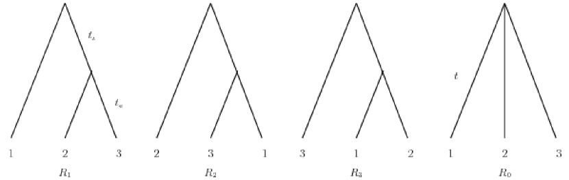
Figure 1. The four rooted trees for three species.

We assume that the sequences evolve according to a two-state continuous-time Markov process with equal substitution rates (which we may take to equal $1$) between the two character states.

Four site patterns can occur. The first one, denoted by $s_{0}$, is such that a given site coincides in the three taxa. The three others, denoted by $s_{i}$ with $i$ in $\tau$, are such that a given site coincide in two taxa and is different in the third taxon, which is taxon $i$. In other words, if one writes the site patterns in taxa $1$, $2$ and $3$ in this order and $x$ and $y$ for any two different characters,

$$s_{0}=xxx,\quad s_{1}=yxx,\quad s_{2}=xyx,\quad\mbox{and}\quad s_{3}=xxy.$$

Let $\{s_{0},s_{1},s_{2},s_{3}\}$ denote the set of site patterns in the specific case described above of three taxa and two states evolving in a two-state symmetric model. Assume that the counting of site pattern $s_{i}$ is $n_{i}$. Then $n=n_{0}+n_{1}+n_{2}+n_{3}$ is the total length of the sequences and, in the independent two-state symmetric model considered in this paper, the quadruple $(n_{0},n_{1},n_{2},n_{3})$ is a sufficient statistics of the sequence data. We use the letter $\mathfrak{n}$ to denote any quadruple $(n_{0},n_{1},n_{2},n_{3})$ of nonnegative integers such that $|\mathfrak{n}|=n_{0}+n_{1}+n_{2}+n_{3}=n\geqslant 1$.

For every site pattern $s_{i}$ and every branch lengths $(t_{\mathrm{e}},t_{\mathrm{i}})$, let $p_{i}(t_{\mathrm{e}},t_{\mathrm{i}})$ denote the probability that $s_{i}$ occurs on tree $R_{1}$ with branch lengths $(t_{\mathrm{e}},t_{\mathrm{i}})$. Standard computations provided by Yang and Rannala [7] show that

$$4p_{0}(t_{\mathrm{e}},t_{\mathrm{i}}) =1+\mathrm{e}^{-4t_{\mathrm{e}}}+2\mathrm{e}^{-4(t_{\mathrm{i}}+t_{\mathrm{e}})},$$

$$4p_{1}(t_{\mathrm{e}},t_{\mathrm{i}}) =1+\mathrm{e}^{-4t_{\mathrm{e}}}-2\mathrm{e}^{-4(t_{\mathrm{i}}+t_{\mathrm{e}})},$$

$$4p_{2}(t_{\mathrm{e}},t_{\mathrm{i}}) =4p_{3}(t_{\mathrm{e}},t_{\mathrm{i}})=1-\mathrm{e}^{-4t_{\mathrm{e}}}.$$

Let $\mathfrak{T}=(T_{\mathrm{e}},T_{\mathrm{i}})$ denote a pair of positive random variables representing the branch lengths $(t_{\mathrm{e}},t_{\mathrm{i}})$, and $\mathfrak{N}=(N_{0},N_{1},N_{2},N_{3})$ denote a quadruple of integer random variables representing the counts of sites patterns $\mathfrak{n}=(n_{0},n_{1},n_{2},n_{3})$.

2. The star tree paradox

Assuming that every taxon evolved from a common ancestor, the aim of phylogeny reconstruction is to compute the most likely tree $R_{i}$. To do so, in the Bayesian approach, one places prior distributions on the trees $R_{i}$ and on their branch lengths $\mathfrak{T}=(T_{\mathrm{e}},T_{\mathrm{i}})$.

2.1. Main result

Let ${\mathbb{P}}(\mathfrak{N}=\mathfrak{n}|R_{i},\mathfrak{T})$ denote the probability that $\mathfrak{N}=\mathfrak{n}$ assuming that the data is generated along the tree $R_{i}$ conditionally on the branch lengths $\mathfrak{T}=(T_{\mathrm{e}},T_{\mathrm{i}})$. One may consider $R_{1}$ only since, for every $\mathfrak{n}=(n_{0},n_{1},n_{2},n_{3})$, the symmetries of the setting yield the relations

$${\mathbb{P}}(\mathfrak{N}=\mathfrak{n}|R_{2},\mathfrak{T})={\mathbb{P}}(\mathfrak{N}=(n_{0},n_{2},n_{3},n_{1})|R_{1},\mathfrak{T}),$$

and

$${\mathbb{P}}(\mathfrak{N}=\mathfrak{n}|R_{3},\mathfrak{T})={\mathbb{P}}(\mathfrak{N}=(n_{0},n_{3},n_{1},n_{2})|R_{1},\mathfrak{T}).$$

Notation 2.1.

For every site pattern $s_{i}$, let $P_{i}$ denote the random variable

$$P_{i}=p_{i}(\mathfrak{T})=p_{i}(T_{\mathrm{e}},T_{\mathrm{i}}).$$

For every $i$ in $\tau$ and every $\mathfrak{n}$, let $\Pi_{i}(\mathfrak{n})$ denote the random variable

$$\Pi_{i}(\mathfrak{n})=P_{0}^{n_{0}}P_{1}^{n_{i}}P_{2}^{n_{j}+n_{k}},\quad\mbox{with}\quad\{i,j,k\}=\tau.$$

We recall that $P_{2}=P_{3}$ and we note that, if $|\mathfrak{n}|=n_{0}+n_{1}+n_{2}+n_{3}=n$ with $n\geqslant 1$, then, for every $i$ in $\tau$,

$$\Pi_{i}(\mathfrak{n})=P_{0}^{n_{0}}P_{1}^{n_{i}}P_{2}^{n-n_{0}-n_{i}}.$$

Fix $\mathfrak{n}$ and assume that $|\mathfrak{n}|=n_{0}+n_{1}+n_{2}+n_{3}=n$ with $n\geqslant 1$. For every $i$ in $\tau$, the posterior probability of $R_{i}$ conditionally on $\mathfrak{N}=\mathfrak{n}$ is

$${\mathbb{P}}(R_{i}|\mathfrak{N}=\mathfrak{n})=\frac{n!}{n_{0}!n_{1}!n_{2}!n_{3}!}\,\frac{1}{{\mathbb{P}}(\mathfrak{N}=\mathfrak{n})}\,{\mathbb{E}}(\Pi_{i}(\mathfrak{n})).$$

Thus, for every $i$ and $j$ in $\tau$,

$$\frac{{\mathbb{P}}(R_{i}|\mathfrak{N}=\mathfrak{n})}{{\mathbb{P}}(R_{j}|\mathfrak{N}=\mathfrak{n})}=\frac{{\mathbb{E}}(\Pi_{i}(\mathfrak{n}))}{{\mathbb{E}}(\Pi_{j}(\mathfrak{n}))}.$$

For every $\varepsilon>0$ and every $i$ in $\tau$, let $\mathscr{N}_{i}^{\varepsilon}$ denote the set of $\mathfrak{n}$ such that, for both indices $j$ in $\tau$ such that $j\neq i$,

$${\mathbb{E}}(\Pi_{i}(\mathfrak{n}))\geqslant(2/\varepsilon)\,{\mathbb{E}}(\Pi_{j}(\mathfrak{n})).$$

One sees that, for every $i$ in $\tau$ and $\mathfrak{n}$ in $\mathscr{N}_{i}^{\varepsilon}$,

$${\mathbb{P}}(R_{i}|\mathfrak{N}=\mathfrak{n})\geqslant 1-\varepsilon,$$

which means that the posterior probability of tree $R_{i}$ among the three possible trees is highly supported.

Recall that, under hypothesis $R_{0}$ and for a tame prior distribution on $\mathfrak{T}=(T_{\mathrm{e}},T_{\mathrm{i}})$, Steel and Matsen prove that, for every $i$ in $\tau$, ${\mathbb{P}}(\mathfrak{N}\in\mathscr{N}_{i}^{\varepsilon})$ does not go to $0$ when the sequence length $n$ goes to infinity, and consequently that the posterior probability ${\mathbb{P}}(R_{i}|\mathfrak{N})$ can be close to $1$ even when the sequence length $n$ is large.

As stated in the introduction, our aim is to prove the same result for tempered prior distributions of $\mathfrak{T}=(T_{\mathrm{e}},T_{\mathrm{i}})$, which we now define.

Notation 2.2.

(1) For every $s\in[0,1]$ and $z\in[0,3]$, let

$$G(z,s)={\mathbb{P}}\left(\mathrm{e}^{-4T_{\mathrm{e}}}(1-\mathrm{e}^{-4T_{\mathrm{i}}})\leqslant s\,|\,\mathrm{e}^{-4T_{\mathrm{e}}}(1+2\mathrm{e}^{-4T_{\mathrm{i}}})=z\right).$$

(2) For every positive $t$ and every site pattern $s_{i}$, let $q_{i}$ denote the probability that $s_{i}$ occurs on tree $R_{0}$, hence

$$4q_{0}=4p_{0}(0,t)=1+3\mathrm{e}^{-4t},\quad 4q_{1}=4q_{2}=4q_{3}=1-\mathrm{e}^{-4t}.$$

(3) Let $\ell_{t}$ denote a positive real number such that $1<4q_{0}-\ell_{t}$ and $4q_{0}+\ell_{t}<4$, for instance $\ell_{t}=3\mathrm{e}^{-4t}\,(1-\mathrm{e}^{-4t})$. Let $I$ and $I_{t}$ denote the intervals

$$I=[0,3],\quad I_{t}=[4q_{0}-1-\ell_{t},4q_{0}-1+\ell_{t}]\subset]0,3[.$$

(4) For every positive $t$ and integer $n$, let

$$Q_{n}(t)={\mathbb{P}}\left(T_{\mathrm{i}}\leqslant 1/n,\,t\leqslant T_{\mathrm{e}}\leqslant t+1/n\right).$$

Definition 2.3 (Tempered priors).

The distribution of $\mathfrak{T}=(T_{\mathrm{e}},T_{\mathrm{i}})$ is tempered if the following two conditions hold.

1. For every $t$, there exists a real number $s_{0}$ in $]0,1]$, an interval $I_{t}$ around $4q_{0}-1$, some bounded functions $F_{i}$, some positive numbers $\alpha$ and $\kappa$, an integer $k\geqslant 1$ and some real numbers $\varepsilon_{i}$ such that

   $$0=\varepsilon_{0}<\varepsilon_{1}<\dots<\varepsilon_{k-1}\leqslant 2<\varepsilon_{k},$$

   and such that for every $s$ in $[0,s_{0}]$ and every $z$ in $I_{t}$,

   $$\left|G(z,s)-\sum_{i=0}^{k-1}F_{i}(z)s^{\alpha+\varepsilon_{i}}\right|\leqslant\kappa s^{\alpha+\varepsilon_{k}}.$$

2. For every positive $t$, $n^{-1}\log Q_{n}(t)\to 0$ when $n\to\infty$.

We detail the properties involved in Definition 2.3 and provide examples of tempered priors in subsection 2.2 below.

We now state our main result, which is an extension of Steel and Matsen’s result to our more general setting.

Theorem 2.4.

Consider sequences of length $n$ generated by a star tree $R_{0}$ on $3$ taxa with strictly positive edge length $t$. Let $\mathfrak{N}$ be the resulting data, summarized by site pattern counts. Consider any prior on the three resolved trees $(R_{1},R_{2},R_{3})$ which assigns strictly positive probability to each tree, and a tempered prior distribution on their branch lengths $\mathfrak{T}=(T_{\mathrm{e}},T_{\mathrm{i}})$.
Then, for every $i$ in $\tau$ and every positive $\varepsilon$, there exists a positive $\delta$ such that, when $n$ is large enough,

$${\mathbb{P}}\left({\mathbb{P}}(R_{i}|\mathfrak{N})\geqslant 1-\varepsilon\right)\geqslant\delta.$$

We prove Theorem 2.4 in Section 4.

2.2. Motivation and intuitive understanding of Definition 2.3

In Definition 2.3, condition 2 is easy to describe, to illustrate and to check, while the content of condition 1 might be more difficult to grasp. Condition 1 involves a Taylor expansion around $s=0$ of the conditional cumulative distribution function $s\mapsto G(z,s)$, where the Taylor coefficients depend on $z$. Such a Taylor expansion roughly describes the prior distribution when $t_{\mathrm{i}}\to 0$ and when $t_{\mathrm{e}}$ is roughly constant. The precise definition of $G(z,\cdot)$ and the technical result stated in Proposition 3.2 are both dictated by our approach to the proof of Theorem 2.4. A key hypothesis is that $\varepsilon_{0}=0$ while $\varepsilon_{k}>2$, which means that we are given a limited expansion of $s\mapsto G(z,s)$ up to a better order than $s^{2}$ when $s\to 0$.

At this point, the reader can wonder how to check if a given prior is tempered or not and if the verification is simply possible in concrete cases, given the convoluted aspect of this definition. Hence we now present some explicit examples of tempered priors. We begin with the following result.

Proposition 2.5.

Assume that $\mathfrak{T}=(T_{\mathrm{e}},T_{\mathrm{i}})$ has a smooth joint probability density, bounded and everywhere non zero. Then the distribution of $\mathfrak{T}=(T_{\mathrm{e}},T_{\mathrm{i}})$ is tempered.

As a consequence, every tame prior fulfills the hypothesis of Proposition 2.5, hence every tame prior is tempered, as claimed in the introduction. This case includes the exponential priors discussed in [7]. We prove Proposition 2.5 in Appendix A.

However some tempered priors are not tame, as illustrated by the following example where Steel and Matsen’s condition fails.

Definition 2.6.

Let $a>0$ and $b>0$. Let $(t_{n})$, $(y_{n})$ and $(r_{n})$ denote sequences of positive numbers, indexed by $n\geqslant 1$ and defined by the formulas

$$t_{n}=n^{-a},\quad y_{n}=1+2\mathrm{e}^{-4t_{n}}\quad r_{n}=y_{n}\,\left(n^{-b}-(n+1)^{-b}\right).$$

Finally, let

$$r=\sum_{n\geqslant 1}r_{n}.$$

Proposition 2.7.

In the setting of Definition 2.6, assume the following:

• $3a<\min\{1,b\}$.

• The random variable $T_{\mathrm{i}}$ is discrete and such that, for every $n\geqslant 1$,

  $${\mathbb{P}}(T_{\mathrm{i}}=t_{n})=r_{n}/r.$$

• The random variable $T_{\mathrm{e}}$ is continuous, independent of $T_{\mathrm{i}}$, with exponential law of parameter $4$, that is, with density $4\,\mathrm{e}^{-4t}$ on $t\geqslant 0$ with respect to the Lebesgue measure.

Then, the distribution of $\mathfrak{T}=(T_{\mathrm{e}},T_{\mathrm{i}})$ is not tame but it is tempered, for the parameters

$$k=3,\quad\alpha=b/a,\quad\varepsilon_{1}=1,\quad\varepsilon_{2}=2,\quad\varepsilon_{3}=3.$$

Since the distribution of $T_{\mathrm{i}}$ is an accumulation of Dirac masses, the prior distribution of $\mathfrak{T}=(T_{\mathrm{e}},T_{\mathrm{i}})$ cannot be tame.

Yet, the fact that the prior distribution is tempered does not come only from the fact that the distribution of $T_{\mathrm{i}}$ is discrete. For a degenerate example, if $T_{\mathrm{i}}=0$ almost surely, then $G(z,s)=1$ for every $s\geqslant 0$, and $G(z,\cdot)$ has no Taylor expansion around zero whose first term is a positive power of $s$. Note that in this particular case, the Bayesian star paradox does not occur.

However, under the conditions of Proposition 2.7, $G(z,\cdot)$ has a Taylor expansion at $0$ fulfilling condition 1 of Definition 2.3. We prove this in Appendix A.

We provide below some examples of less ill-behaved distributions which are tempered but not tame, and an example of a distribution which does not fulfill condition 1, hence is not tempered.

Proposition 2.8.

Assume that $T_{\mathrm{e}}$ is a continuous random variable, with exponential law of parameter $4$, that is, with density $4\,\mathrm{e}^{-4t}$ on $t\geqslant 0$ with respect to the Lebesgue measure, and that $T_{\mathrm{i}}$ is a random variable independent of $T_{\mathrm{e}}$. Then, the following holds.

• If the distribution of $T_{\mathrm{i}}$ is uniform on $[0,\theta]$, with $\theta>0$, the distribution of $\mathfrak{T}=(T_{\mathrm{e}},T_{\mathrm{i}})$ is tempered but not tame.

• If the distribution of $T_{\mathrm{i}}$ has density $\theta t_{\mathrm{i}}^{\theta-1}$ on the interval $[0,1]$, for a given $\theta$ in $(0,1)$, the distribution of $\mathfrak{T}=(T_{\mathrm{e}},T_{\mathrm{i}})$ is tempered but not tame.

• If the distribution of $T_{\mathrm{i}}$ has density $\log(1/t_{\mathrm{i}})$ on the interval $[0,1]$, the distribution of $\mathfrak{T}=(T_{\mathrm{e}},T_{\mathrm{i}})$ is not tempered.

• If the distribution of $T_{\mathrm{i}}$ has density $4\,t_{\mathrm{i}}\log(1/t_{\mathrm{i}})$ on the interval $[0,1]$, the distribution of $\mathfrak{T}=(T_{\mathrm{e}},T_{\mathrm{i}})$ is not tempered.

Note that in case $(iv)$, the density function of $\mathfrak{T}=(T_{\mathrm{e}},T_{\mathrm{i}})$ is bounded, non smooth but continuous, but the distribution is not tempered.

We prove Proposition 2.8 in Appendix A.

3. Extension of Steel and Matsen’s lemma

The Bayesian star paradox due to Steel and Matsen relies on a technical result which we slightly rephrase as follows. For every nonnegative real $t$ and every $[0,1]$ valued random variable $V$, introduce

$$M_{t}={\mathbb{E}}(V^{t}),\quad R_{t}=1-\frac{M_{t+1}}{M_{t}}=\frac{{\mathbb{E}}\left(V^{t}(1-V)\right)}{{\mathbb{E}}(V^{t})}.$$

Proposition 3.1 (Steel and Matsen’s lemma).

Let $0\leqslant\eta<1$ and $B>0$. There exists a finite $K$, which depends on $\eta$ and $B$ only, such that the following holds. For every $[0,1]$ valued random variable $V$ with a smooth probability density function $f$ such that $f(1)>0$ and $|f^{\prime}(v)|\leqslant Bf(1)$ for every $\eta\leqslant v\leqslant 1$, and for every integer $k\geqslant K$,

$$2kR_{k}\geqslant 1.$$

Indeed the asymptotics of $R_{k}$ when $k$ is large depends on the behaviour of the distribution of $V$ around $1$.

Our next proposition proves that the conclusion of Steel and Matsen’s lemma above holds for a wider class of random variables.

Proposition 3.2.

Let $V$ a random variable on $[0,1]$. Suppose that there exists an integer $n\geqslant 1$ and real numbers $0\leqslant v_{0}<1$, $\alpha>0$, $\varepsilon_{i}$ and $\gamma_{i}$, such that

$$0=\varepsilon_{0}<\varepsilon_{1}<\dots<\varepsilon_{n-1}\leqslant 1<\varepsilon_{n},$$

and, for every $v_{0}\leqslant v\leqslant 1$,

$$\left|{\mathbb{P}}(V\geqslant v)-\sum_{i=0}^{n-1}\gamma_{i}(1-v)^{\alpha+\varepsilon_{i}}\right|\leqslant\gamma_{n}(1-v)^{\alpha+\varepsilon_{n}}.$$

Then there exists a finite $\theta(\gamma)$, which depends continuously on $\gamma=(\gamma_{0},\ldots,\gamma_{n})$, such that for every $t\geqslant\theta(\gamma)$,

$$2tR_{t}\geqslant\alpha.$$

Remark 1.

We insist on the fact that $\theta(\gamma)$ depends continuously on the multiparameter $\gamma=(\gamma_{0},\ldots,\gamma_{n})$. To wit, in the proof of Proposition 5.6, we apply Proposition 3.2 with bounded functions of $z$. This means that for every $z$ in $I_{t}$, one gets a number $\theta$ which depends on $z$ through the bounded functions such that the control on the distribution of $V$ holds. The continuity of $\theta$ ensures that there exists a number independent of $z$ such that Proposition 5.6 holds.

Remark 2.

If one computes a Taylor expansion of the function $v\mapsto{\mathbb{P}}(V\geqslant v)$ at $v=1^{-}$ under the conditions of Steel and Matsen’s lemma, one sees that conditions of Proposition 3.2 hold. Hence Proposition 3.2 is an extension of Steel and Matsen’s lemma.

We prove Proposition 3.2 in Appendix B. The proof of Theorem 2.4 relies on it.

4. Synopsis of the proof of Theorem 2.4

This section is devoted to a sketch of the proof of Theorem 2.4. We use the definitions below. Note that the set $F_{c}^{(n)}$ defined below is not the set introduced by Steel and Matsen. For a technical reason in the proof of Proposition 4.2 stated below, we had to modify their definition. Note however that Propositions 4.2 and 4.3 below are adaptations of ideas in Steel and Matsen’s paper.

Notation 4.1.

Define functions $\Delta_{i}$ as follows. For every nonnegative integers $\mathfrak{n}=(n_{0},n_{1},n_{2},n_{3})$ such that $|\mathfrak{n}|=n_{0}+n_{1}+n_{2}+n_{3}=n$ with $n\geqslant 1$,

$$\Delta_{0}(\mathfrak{n})=\frac{n_{0}-q_{0}n}{\sqrt{n}},$$

and, for every $i$ in $\tau$,

$$\Delta_{i}(\mathfrak{n})=\frac{n_{i}-1/3(n-n_{0})}{\sqrt{n}}.$$

For every $c>1$, introduce

$$F_{c}^{(n)}=\{\mathfrak{n}\,;\,|\mathfrak{n}|=n,\,-2c\leqslant\Delta_{2}(\mathfrak{n})\leqslant-c,\,-2c\leqslant\Delta_{3}(\mathfrak{n})\leqslant-c,\,-c\leqslant\Delta_{0}(\mathfrak{n})\leqslant 0\}.$$

For every $i$ in $\tau$ and every positive $\eta$, let $A^{i}_{\eta}$ denote the event

$$A^{i}_{\eta}=\left\{\forall j\in\tau,\,j\neq i,\,{\mathbb{E}}(\Pi_{i}(N)\,|\,N)\geqslant\eta{\mathbb{E}}(\Pi_{j}(N)\,|\,N)\right\}.$$

Since $\Delta_{1}+\Delta_{2}+\Delta_{3}=0$, every $\mathfrak{n}$ in $F_{c}^{(n)}$ is such that $2c\leqslant\Delta_{1}(\mathfrak{n})\leqslant 4c$. We note that $F_{c}^{(n)}$ is not symmetric about $\tau$ and gives a preference to $1$. That is why we only deal with $A^{1}_{\eta}$ in the following proof. To deal with $A^{i}_{\eta}$, one would change the definition $F_{c}^{(n)}$ accordingly.

From the reasoning in Section 2, it suffices to prove that for every positive $\eta$, there exists a positive $\delta$ such that, when $n$ is large enough,

$${\mathbb{P}}\left(A^{1}_{\eta}\right)\geqslant\delta.$$

Suppose that one generates $n\geqslant 1$ sites on the star tree $R_{0}$ with given branch length $t$ and let $\mathfrak{N}=(N_{0},N_{1},N_{2},N_{3})$ denote the counts of site patterns defined in Section 1, hence $N_{0}+N_{1}+N_{2}+N_{3}=n$.

From central limit estimates, the probability of the event $\left\{\mathfrak{N}\in F_{c}^{(n)}\right\}$ is uniformly bounded from below, say by $\delta>0$, when $n$ is large enough. Hence,

$${\mathbb{P}}\left(A^{1}_{\eta}\right)\geqslant\delta{\mathbb{P}}\left(A^{1}_{\eta}\big{|}\,\mathfrak{N}\in F_{c}^{(n)}\right)$$

We wish to prove that there exists a positive $\alpha$ independent of $c$ such that for $n$ large enough and for every $\mathfrak{n}$ in $F_{c}^{(n)}$ and for $j=2$ and $j=3$,

$${\mathbb{E}}(\Pi_{1}(\mathfrak{n}))\geqslant c^{2}\alpha\,{\mathbb{E}}(\Pi_{j}(\mathfrak{n})).$$

This follows from the two results below, adapted from Steel and Matsen’s paper.

Proposition 4.2.

Fix $t$ and assume that $\mathfrak{n}$ is in $F_{c}^{(n)}$. Then, when $n$ is large enough, for $j=2$ and $j=3$,

$${\mathbb{E}}(\Pi_{j}(\mathfrak{n})\,|\,4P_{0}-1\in I_{t})\geqslant{\mathbb{E}}(\Pi_{j}(\mathfrak{n})\,|\,4P_{0}-1\notin I_{t}).$$

Proposition 4.3.

Fix $t$ and assume that $\mathfrak{n}$ is in $F_{c}^{(n)}$. Then, there exists a positive $\alpha$, independent of $c$, such that for every $z$ in $I_{t}$, and for $j=2$ and $j=3$,

$${\mathbb{E}}(\Pi_{1}(\mathfrak{n})\,|\,4P_{0}-1=z)\geqslant c^{2}\alpha{\mathbb{E}}(\Pi_{j}(\mathfrak{n})\,|\,4P_{0}-1=z).$$

We prove Propositions 4.2 and 4.3 in Section 5.

From these two results, for $j=2$ and $j=3$,

$${\mathbb{E}}(\Pi_{1}(\mathfrak{n}))\geqslant c^{2}\alpha{\mathbb{P}}(4P_{0}-1\in I_{t})\,{\mathbb{E}}(\Pi_{j}(\mathfrak{n})).$$

Assume that $c$ is so large that $c^{2}\alpha{\mathbb{P}}(4P_{0}-1\in I_{t})\geqslant\eta$. Then, for every $\mathfrak{n}$ in $F_{c}^{(n)}$ and for $j=2$ and $j=3$,

$${\mathbb{E}}(\Pi_{1}(\mathfrak{n}))\geqslant\eta\,{\mathbb{E}}(\Pi_{j}(\mathfrak{n})).$$

This implies that ${\mathbb{P}}\left(A^{1}_{\eta}\big{|}\,\mathfrak{N}\in F_{c}^{(n)}\right)=1,$ which yields the theorem.

5. Proofs of Propositions 4.2 and 4.3

5.1. Proof of Proposition 4.2

The proof is decomposed into two intermediate results, stated as lemmata below and using estimates on auxiliary random variables introduced below.

Notation 5.1.

For every $n\geqslant 1$ and $t>0$, let $\Gamma_{t}(n)=[0,1/n]\times[t,t+1/n]$.
For every $t>0$, let $\mu_{t}=q_{0}^{q_{0}}q_{1}^{q_{1}}q_{2}^{q_{2}}q_{3}^{q_{3}}=q_{0}^{q_{0}}q_{1}^{3q_{1}}$ and $U_{t}$ denote the random variable

$$U_{t}=\prod_{i=0}^{3}(P_{i}/q_{i})^{q_{i}}.$$

For every $\mathfrak{n}$ and for $j=2$ and $j=3$, let $W_{j}(\mathfrak{n})$ denote the random variable

$$W_{j}(\mathfrak{n})=P_{0}^{\Delta_{0}(\mathfrak{n})}P_{1}^{(\Delta_{j}-\Delta_{0}/3)(\mathfrak{n})}P_{2}^{(\Delta_{1}+\Delta_{k}-2\Delta_{0}/3)(\mathfrak{n})},\quad\mbox{with}\quad\{j,k\}=\{2,3\}.$$

One sees that

$$U_{t}=P_{0}^{q_{0}}P_{1}^{q_{1}}P_{2}^{2q_{1}}/\mu_{t},\qquad Q_{n}(t)={\mathbb{P}}\left(\mathfrak{T}\in\Gamma_{t}(n)\right),$$

and, for $j=2$ and $j=3$,

$$W_{j}=(P_{0}/P_{2})^{\Delta_{0}}(P_{1}/P_{2})^{\Delta_{j}-\Delta_{0}/3}.$$

Lemma 5.2.

(1) For every $\mathfrak{n}$ in $F_{c}^{(n)}$ and for $j=2$ and $j=3$, $W_{j}(\mathfrak{n})\leqslant 1$.
(2) For every $\mathfrak{n}$ in $F_{c}^{(n)}$ and for $j=2$ and $j=3$, $W_{j}(\mathfrak{n})\geqslant(q_{1})^{c}$ on the event $\{\mathfrak{T}\in\Gamma_{t}(n)\}$.
(3) There exists a finite constant $\kappa$ such that $U_{t}^{n}\geqslant\mathrm{e}^{-\kappa}$ uniformly on the integer $n\geqslant 1$ and on the event $\{\mathfrak{T}\in\Gamma_{t}(n)\}$.

Proof of Lemma 5.2.

(1) For every $\mathfrak{T}$, $P_{0}\geqslant P_{1}\geqslant P_{2}$. On $F_{c}^{(n)}$, $\Delta_{0}\leqslant 0$ and for $j=2$ and $j=3$, $\Delta_{j}-\Delta_{0}/3\leqslant 0$ hence

$$(P_{0}/P_{1})^{\Delta_{0}}\leqslant 1,\quad(P_{0}/P_{2})^{\Delta_{j}-\Delta_{0}/3}\leqslant 1.$$

This proves the claim.

(2) One has $P_{0}\leqslant 1$ everywhere and $P_{1}\geqslant q_{1}$ and $P_{2}\geqslant q_{1}$ on the event $\{\mathfrak{T}\in\Gamma_{t}(n)\}$. On $F_{c}^{(n)}$, $\Delta_{0}\leqslant 0$ and for $j=2$ and $j=3$, $\Delta_{j}-\Delta_{0}/3\leqslant 0$ hence $W_{j}\geqslant q_{2}^{-\Delta_{j}-2\Delta_{0}/3}$. Finally, on $F_{c}^{(n)}$, $\Delta_{j}+2\Delta_{0}/3\leqslant-c$. This proves the claim.

(3) For every $\mathfrak{T}$ in $\Gamma_{t}(n)$, one has $T_{\mathrm{i}}\geqslant 0$ and $T_{\mathrm{e}}\geqslant t$, hence $P_{1}\geqslant q_{1}$ and $P_{2}\geqslant q_{2}=q_{1}$. Likewise, $T_{\mathrm{i}}\leqslant 1/n$ and $T_{\mathrm{e}}\leqslant t+1/n$ hence

$$P_{0}\geqslant p_{0}(1/n,t+1/n)\geqslant q_{0}-5\mathrm{e}^{-4t}(1-\mathrm{e}^{-4/n})/4.$$

This yields that, for every $n\geqslant 1$ and every $\mathfrak{T}$ in $\Gamma_{t}(n)$,

$$U_{t}^{n}\geqslant(1-5\mathrm{e}^{-4t}/(q_{0}n))^{n}\to\exp(-5\mathrm{e}^{-4t}/q_{0})>0,$$

which implies the desired lower bound. ∎

Lemma 5.3.

For every $\mathfrak{n}$ in $F_{c}^{(n)}$ and for $j=2$ and $j=3$,

$${\mathbb{E}}(\Pi_{j}(\mathfrak{n})\,|\,4P_{0}-1\in I_{t})\geqslant\mu_{t}^{n}Q_{n}(t)\exp(-O(\sqrt{n})),$$

and

$${\mathbb{E}}(\Pi_{j}(\mathfrak{n})\,|\,4P_{0}-1\notin I_{t})\leqslant\mu_{t}^{n}\exp(-n\ell_{t}^{2}/32).$$

Proof of Lemma 5.3.

Since $P_{0}=p_{0}(\mathfrak{T})$, for every $\mathfrak{T}$ in $\Gamma_{t}(n)$, when $n$ is large, $4P_{0}-1$ is in the interval $I_{t}$. Consequently,

$${\mathbb{E}}(\Pi_{j}(\mathfrak{n})\,|\,4P_{1}-1\in I_{t})\geqslant Q_{n}(t){\mathbb{E}}\left(\Pi_{j}(\mathfrak{n})\,|\,\mathfrak{T}\in\Gamma_{t}(n)\right).$$

On the event $\{\mathfrak{T}\in\Gamma_{t}(n)\}$,

$$\Pi_{j}(\mathfrak{n})=\mu_{t}^{n}U_{t}^{n}W_{j}(\mathfrak{n})^{\sqrt{n}}\geqslant\mu_{t}^{n}\mathrm{e}^{-\kappa}(q_{1})^{c\sqrt{n}},$$

from parts (2) and (3) of Lemma 5.2, which proves the first part of the lemma.

Turning to the second part, let $\mathrm{d}_{KL}$ denote the Kullback-Leibler distance between discrete probability measures. When $4P_{0}-1$ is not in $I_{t}$,

$$\mathrm{d}_{KL}(q,P)\geqslant(1/2)\|q-P\|_{1}^{2}\geqslant(1/2)(q_{0}-P_{0})^{2}\geqslant\ell_{t}^{2}/32.$$

Note that

$$\Pi_{j}(\mathfrak{n})=\mu_{t}^{n}W_{j}(\mathfrak{n})^{\sqrt{n}}\exp(-n\mathrm{d}_{KL}(q,P)),$$

hence the estimate on $\mathrm{d}_{KL}(q,P)$, and part (1) of Lemma 5.2, imply the second part of the lemma. ∎

Turning finally to the proof of Proposition 4.2, we note that $Q_{n}(t)=\mathrm{e}^{o(n)}$ because the distribution of $\mathfrak{T}$ is tempered. Furthermore, Lemma 5.3 shows that, when $n$ is large enough,

$${\mathbb{E}}(\Pi_{j}(\mathfrak{n})\,|\,4P_{0}-1\in I_{t})\geqslant{\mathbb{E}}(\Pi_{j}(\mathfrak{n})\,|\,4P_{0}-1\notin I_{t}),$$

and this concludes the proof of Proposition 4.2.

5.2. Proof of Proposition 4.3

Our proof of Proposition 4.3 is based on Lemma 5.5 and Proposition 5.6 below.

Notation 5.4.

For every $u$ in $[0,1]$, let $\zeta(u)=(1+2u)(1-u)^{2}$. Let $U$ and $V$ denote the random variables defined as

$$U=(P_{1}-P_{2})/(1-P_{0}),\qquad V=\zeta(U).$$

Lemma 5.5.

For every $\mathfrak{n}$ in $F_{c}^{(n)}$ and for $j=2$ and $j=3$,

$$\frac{{\mathbb{E}}(\Pi_{1}(\mathfrak{n})\,|\,P_{0})}{{\mathbb{E}}(\Pi_{j}(\mathfrak{n})\,|\,P_{0})}\geqslant 4c^{2}n\frac{{\mathbb{E}}\left(V^{s}(1-V)\,|\,P_{0}\right)}{{\mathbb{E}}\left(V^{s}\,|\,P_{0}\right)},\quad\mbox{where}\ s=(n-n_{0})/3.$$

Proof of Lemma 5.5.

Recall that, for every $c>1$, $F_{c}^{(n)}$ is

$$F_{c}^{(n)}=\{\mathfrak{n}\,:\,|\mathfrak{n}|=n,\,-2c\leqslant\Delta_{2}(\mathfrak{n})\leqslant c,-2c\leqslant\Delta_{3}(\mathfrak{n})\leqslant c,-c\leqslant\Delta_{0}(\mathfrak{n})\leqslant 0\}.$$

Using the $\Delta$ variables, one can rewrite $\Pi_{1}$, $\Pi_{2}$ and $\Pi_{3}$ as

$$\Pi_{i}(\mathfrak{n})=P_{0}^{n_{0}}(P_{1}P_{2}^{2})^{s}\left(P_{1}/P_{2}\right)^{\Delta_{i}(\mathfrak{n})\sqrt{n}},\quad i=1,2,3,\ s=(n-n_{0})/3.$$

Assume that $\mathfrak{n}$ is in $F_{c}^{(n)}$. Then, $\Delta_{1}(\mathfrak{n})\geqslant 2c$, $\Delta_{j}(\mathfrak{n})\leqslant 0$ for $j=2$ and $j=3$, and $P_{1}\geqslant P_{2}$. Hence

$$\Pi_{1}(\mathfrak{n})\geqslant P_{0}^{n_{0}}(P_{1}P_{2}^{2})^{s}\left(P_{1}/P_{2}\right)^{2c\sqrt{n}},\qquad\Pi_{j}(\mathfrak{n})\leqslant P_{0}^{n_{0}}(P_{1}P_{2}^{2})^{s}.$$

Furthermore,

$$P_{1}P_{2}^{2}=(1/27)V(1-P_{0})^{3},\quad P_{1}/P_{2}=(1+2U)/(1-U),$$

hence for $j=2$ and $j=3$,

$$\frac{{\mathbb{E}}(\Pi_{1}(\mathfrak{n})\,|\,P_{0})}{{\mathbb{E}}(\Pi_{j}(\mathfrak{n})\,|\,P_{0})}\geqslant\frac{{\mathbb{E}}\left(V^{s}\left((1+2U)/(1-U)\right)^{2c\sqrt{n}}\,|\,P_{0}\right)}{{\mathbb{E}}\left(V^{s}\,|\,P_{0}\right)}.$$

Direct computations (or Lemma 3.2 in Steel and Matsen [3]) show that, for every $u$ in $[0,1)$ and every $m\geqslant 3$,

$$\left((1+2u)/(1-u)\right)^{m}\geqslant m^{2}(1-\zeta(u)),$$

hence

$$\left((1+2U)/(1-U)\right)^{2c\sqrt{n}}\geqslant 4c^{2}n\,(1-V).$$

The conclusion of Lemma 5.5 follows. ∎

Proposition 5.6.

Assume that the distribution of $\mathfrak{T}$ is tempered. Then there exists $\theta$ and $\alpha$, both positive and independent of $c$, such that for every $s\geqslant\theta$, on the event $\{4P_{0}-1\in I_{t}\}$,

$$4s\,{\mathbb{E}}(V^{s}(1-V)\,|\,P_{0})\geqslant\alpha\,{\mathbb{E}}(V^{s}\,|\,P_{0}).$$

Proof of Proposition 5.6.

We recall that $U$ and $V$ denote random variables defined as

$$U=(P_{1}-P_{2})/(1-P_{0}),\quad V=\zeta(U),\quad\zeta(u)=(1+2u)(1-u)^{2}.$$

To use Proposition 3.2, one must compute a Taylor expansion at $v=1^{-}$ or, equivalently, at $u=0^{+}$, of the conditional probability

$${\mathbb{P}}(V\geqslant v\,|\,P_{0})={\mathbb{P}}(U\leqslant u\,|\,P_{0}),$$

where $u=\zeta^{-1}(v)$. Besides, for $v$ close to $1$,

$$u=\zeta^{-1}(v)=w/\sqrt{3}+w^{2}/9+5w^{3}/54\sqrt{3}+O(w^{4}),\quad\mbox{with }w=\sqrt{1-v}.$$

Since $U=(P_{1}-P_{2})/(1-P_{0})$,

$${\mathbb{P}}(U\leqslant u\,|\,4P_{0}-1=z)={\mathbb{P}}\left(S_{\mathrm{e}}(3-S_{\mathrm{i}})\leqslant 2s\,|\,S_{\mathrm{e}}S_{\mathrm{i}}=z\right),$$

where we used the notations

$$S_{\mathrm{e}}=\mathrm{e}^{-4T_{\mathrm{e}}},\quad S_{\mathrm{i}}=1+2\mathrm{e}^{-4T_{\mathrm{i}}},\quad 2s=u(3-z).$$

Using Definition 2.3, one has

$$G(z,s)={\mathbb{P}}\left(S_{\mathrm{e}}(3-S_{\mathrm{i}})\leqslant 2s\,|\,S_{\mathrm{e}}S_{\mathrm{i}}=z\right).$$

Since the distribution of $\mathfrak{T}$ is tempered, there exists some bounded functions $F_{i}$ defined on $I_{t}$, a positive number $\alpha$, $n+1$ real numbers

$$0=\varepsilon_{0}<\varepsilon_{1}<\dots<\varepsilon_{n-1}\leqslant 2<\varepsilon_{n},$$

and two positive numbers $\kappa$ and $s_{0}$ such that for every $0\leqslant s\leqslant s_{0}$ and every $z$ in $I_{t}$,

$$\left|G(z,s)-\sum_{i=0}^{n-1}F_{i}(z)s^{\alpha+\varepsilon_{i}}\right|\leqslant\kappa s^{\alpha+\varepsilon_{n}}.$$

Combining this with the relation $2s=u(3-z)$ and the expansion of $u=\zeta^{-1}(v)$ along the powers of $w$, one sees that there exists some bounded functions $f_{i}$ on $I_{t}$, a positive number $\kappa^{\prime}$ and $0\leqslant v_{0}<1$ such that for every $v_{0}\leqslant v\leqslant 1$ and every $z\in I_{t}$,

$$\left|{\mathbb{P}}(V\geqslant v\,|\,4P_{0}-1=z)-\sum_{i=0}^{n-1}f_{i}(z)(1-v)^{\alpha/2+\varepsilon_{i}/2}\right|\leqslant\kappa^{\prime}(1-v)^{\alpha/2+\varepsilon_{n}/2}.$$

Since the functions $f_{i}$ are bounded and positive on $I_{t}$, Proposition 3.2 implies that there exists a positive number $\theta$ such that for every $z$ in $I_{t}$ and every $s\geqslant\theta$, the conclusion of Proposition 5.6 holds. ∎

Assuming this, the proof of Proposition 4.3 is as follows. Let $s$, $\theta$ and $\alpha$ be as in Lemma 5.5 and Proposition 5.6. Since $n-n_{0}=(1-q_{0})n-\Delta_{0}\sqrt{n}\geqslant(1-q_{0})n$ for every $\mathfrak{n}$ in $F_{c}^{(n)}$, one knows that $s=(n-n_{0})/3\geqslant\theta$ when $n$ is large enough. Furthermore, $s\leqslant n/3$. Finally, for every $\mathfrak{n}$ in $F_{c}^{(n)}$ with $n$ large enough, on the event $\{4P_{0}-1\in I_{t}\}$ and for $j=2$ and $j=3$,

$${\mathbb{E}}(\Pi_{1}(\mathfrak{n})\,|\,P_{0})\geqslant 3c^{2}\alpha\,{\mathbb{E}}(\Pi_{j}(\mathfrak{n})\,|\,P_{0}).$$

This concludes the proof of Proposition 4.3.

Appendix A Proof of Propositions 2.5, 2.7, and 2.8

Notation A.1.

Introduce the random variables

$$(S_{\mathrm{e}},S_{\mathrm{i}})=\varsigma(T_{\mathrm{e}},T_{\mathrm{i}}),\qquad\mbox{where}\ \varsigma(t_{\mathrm{e}},t_{\mathrm{i}})=(\mathrm{e}^{-4t_{\mathrm{e}}},1+2\mathrm{e}^{-4t_{\mathrm{i}}}),$$

that is,

$$S_{\mathrm{e}}=\mathrm{e}^{-4T_{\mathrm{e}}},\qquad S_{\mathrm{i}}=1+2\mathrm{e}^{-4T_{\mathrm{i}}}.$$

Hence, $G(z,\cdot)$ is defined by

$$G(z,s)={\mathbb{P}}\left(3S_{\mathrm{e}}\leqslant 2s+z\,|\,S_{\mathrm{e}}S_{\mathrm{i}}=z\right),$$

A.1. Proof of Proposition 2.5

The distribution of $(S_{\mathrm{e}},S_{\mathrm{i}})$ has a smooth joint probability density, say $\varpi$, defined on the set $0<x\leqslant 1<y\leqslant 3$ by

$$\varpi(x,y)=\frac{\omega\circ\varsigma^{-1}(x,y)}{16x(y-1)}.$$

For tame priors, the probability $Q_{n}(t)$ introduced in condition 2 of Definition 2.3 is of order $1/n^{2}$, hence this condition holds.

The definition of $G(z,s)$ as a conditional expectation can be rewritten as

$$G(z,s)={\mathbb{P}}\left(3S_{\mathrm{e}}\leqslant 2s+S_{\mathrm{e}}S_{\mathrm{i}}\,|\,S_{\mathrm{e}}S_{\mathrm{i}}=z\right).$$

Hence, for every measurable bounded function $H$,

$${\mathbb{E}}\left(H(S_{\mathrm{e}}S_{\mathrm{i}})\,;\,3S_{\mathrm{e}}\leqslant 2s+S_{\mathrm{e}}S_{\mathrm{i}}\right)={\mathbb{E}}\left(H(S_{\mathrm{e}}S_{\mathrm{i}})G(S_{\mathrm{e}}S_{\mathrm{i}},s)\right),$$

that is,

$$\iint H(xy){\mathbf{1}}\{3x\leqslant 2s+xy\}\varpi(x,y)\mathrm{d}x\mathrm{d}y=\iint H(xy)G(xy,s)\varpi(x,y)\mathrm{d}x\mathrm{d}y.$$

The change of variable $z=xy$ yields

$$\iint H(z){\mathbf{1}}\{3x\leqslant 2s+z\}\varpi\left(x,z/x\right)\mathrm{d}z\mathrm{d}x/x=\iint H(z)G(z,s)\varpi\left(x,z/x\right)\mathrm{d}z\mathrm{d}x/x.$$

This must hold for every measurable bounded function $H$, hence one can choose

$$G(z,s)=H(z,s)/H(z,\infty),$$

with

$$H(z,s)=\int{\mathbf{1}}\{3x\leqslant 2s+z\}\varpi\left(x,z/x\right)\mathrm{d}x/x.$$

Since $0\leqslant S_{\mathrm{e}}\leqslant 1\leqslant S_{\mathrm{i}}\leqslant 3$ almost surely, the integral defining $H(z,s)$ may be further restricted to the range $0\leqslant x\leqslant 1$ and $z/3\leqslant x\leqslant z$. Finally, for every $s\geqslant 0$ and $z\in[0,3]$,

$$G(z,s)=H(z,s)/H(z,1),$$

where

$$H(z,s)=\int_{m(0,z)}^{m(s,z)}\varpi\left(x,z/x\right)\mathrm{d}x/x,\quad\mbox{with }m(s,z)=\min\{1,z,(2s+z)/3\}.$$

Hence, $m(0,z)=z/3$ and, for small positive values of $s$, $m(s,z)=m(0,z)+2s/3$. When $0\leqslant z\leqslant 1$, $m(s,z)\to m(\infty,z)=z$ when $s\to\infty$ and this limit is reached for $s=z$. When $1\leqslant z\leqslant 3$, $m(s,z)\to m(\infty,z)=1$ when $s\to\infty$ and this limit is reached for $s=(3-z)/2$. In both cases, $m(\infty,z)=m(1,z)$ hence $H(z,\infty)=H(z,1)$.

Because $\omega$ and $\varsigma^{-1}$ are smooth, the Taylor-Lagrange formula shows that, for every $s\geqslant 0$ and every fixed $z$,

$$H(z,s)=H(z,0)+H^{\prime}(z,0)s+H^{\prime\prime}(z,0)\frac{s^{2}}{2}+H^{(3)}(z,0)\frac{s^{3}}{6}+\int_{0}^{s}(x-s)^{3}H^{(4)}(z,s)\frac{\mathrm{d}x}{24},$$

where all the derivatives are partial derivatives with respect to the second argument $s$.

Simple computations yield $H(z,0)=0$ and the values of the three derivatives $H^{\prime}(z,0)$, $H^{\prime\prime}(z,0)$ and $H^{(3)}(z,0)$ as combinations of $\omega$ and of partial derivatives of $\omega$, evaluated at the point $(\vartheta,0)$, where $3\mathrm{e}^{-4\vartheta}=z$.

Furthermore, the hypothesis on $\omega$ ensures that $H^{(4)}(z,\cdot)$ is bounded, in the following sense: there exist positive numbers $s_{0}$ and $\kappa_{0}$ such that for every $s$ in $[0,s_{0}]$ and every $z$ in $I_{t}$,

$$H^{(4)}(z,s)\leqslant 24\kappa_{0}.$$

Hence, $\mathfrak{T}=(T_{\mathrm{e}},T_{\mathrm{i}})$ fulfills the first condition to be tempered, with

$$k=3,\quad\alpha=1,\quad\varepsilon_{1}=1,\quad\varepsilon_{2}=2,\quad\varepsilon_{3}=3,\quad\kappa=\kappa_{0},$$

and, for every $0\leqslant i\leqslant 2$,

$$F_{i}(z)=H^{(i+1)}(z,0)/H(z,1).$$

Finally, since $\omega$ is smooth, the functions $F_{i}$ are bounded on $I_{t}$.

A.2. Proof of Proposition 2.7

Recall that, using the random variables $S_{\mathrm{e}}=\mathrm{e}^{-4T_{\mathrm{e}}}$ and $S_{\mathrm{i}}=1+2\mathrm{e}^{-4T_{\mathrm{i}}}$, the function $G$ is characterized by the fact that, for every measurable bounded function $H$,

$${\mathbb{E}}\left(H(S_{\mathrm{e}}S_{\mathrm{i}}):S_{\mathrm{e}}(3-S_{\mathrm{i}})\leqslant 2s\right)={\mathbb{E}}\left(H(S_{\mathrm{e}}S_{\mathrm{i}})G(S_{\mathrm{e}}S_{\mathrm{i}},s)\right).$$

Here, $S_{\mathrm{e}}$ and $S_{\mathrm{i}}$ are independent, the distribution of $S_{\mathrm{e}}$ is uniform on $[0,1]$ and the distribution of $S_{\mathrm{i}}$ is discrete with

$${\mathbb{P}}(S_{\mathrm{i}}=y_{n})=r_{n}/r.$$

Thus,

$$\sum_{n}r_{n}\int_{0}^{1}H(xy_{n})\,{\mathbf{1}}\{x(3-y_{n})\leqslant 2s\}\,\mathrm{d}x=\sum_{n}r_{n}\int_{0}^{1}H(xy_{n})\,G(xy_{n},s)\,\mathrm{d}x.$$

The changes of variable $z=y_{n}x$ in each integral yield

$$\sum_{n}\frac{r_{n}}{y_{n}}\int H(z)\,{\mathbf{1}}\{z\leqslant y_{n}\}{\mathbf{1}}\{3z\leqslant(2s+z)y_{n}\}\,\mathrm{d}z=\sum_{n}\frac{r_{n}}{y_{n}}\int H(z)\,{\mathbf{1}}\{z\leqslant y_{n}\}\,G(z,s)\,\mathrm{d}z.$$

This must hold for every measurable bounded function $H$, hence

$$G(z,s)=H(z,s)/H(z,\infty),\quad H(z,s)=\sum_{n}(r_{n}/y_{n})\,{\mathbf{1}}\{z\leqslant y_{n}\}{\mathbf{1}}\{3z\leqslant(2s+z)y_{n}\}.$$

Since $r_{n}/y_{n}=n^{-b}-(n+1)^{-b}$ for $n\geqslant 1$, $H(z,s)=n(z,s)^{-b}$ where

$$n(z,s)=\inf\{n\geqslant 1\,|\,z\leqslant y_{n},\,3z\leqslant(2s+z)y_{n}\}.$$

Since $y_{n}\to 3$ when $n\to\infty$, $n(z,s)$ is finite for every $z<3$ and $s>0$.

For every $z>0$, when $s$ is large enough, namely $s\geqslant(3-z)/2$, the condition that $3z\leqslant(2s+z)y_{n}$ becomes useless and

$$n(z,s)=\inf\{n\geqslant 1\,|\,z\leqslant y_{n}\},$$

hence $n(z,s)$ and $H(z,s)$ are independent of $s$. If $z\geqslant 1$, this implies that $n(z,s)$ and $H(z,s)$ are independent of $s\geqslant 1$. If $z<1$ and $s\geqslant 1$, the conditions that $z\leqslant y_{n}$ and $3z\leqslant(2s+z)y_{n}$ both hold for every $n\geqslant 1$ hence $n(z,s)=1$ and $H(z,s)=1$. In both cases, $H(z,\infty)=H(z,1)$.

We are interested in small positive values of $s$. For every $z<3$, when $s$ is small enough, namely $s\leqslant(3-z)/2$, the condition $z\leqslant y_{n}$ becomes useless and

$$n(z,s)=\inf\{n\geqslant 1\,|\,3z\leqslant(2s+z)y_{n}\},$$

When furthermore $s<z$, $n\geqslant n(z,s)$ is equivalent to the condition

$$n^{-a}\leqslant h(s/z),\quad\mbox{with}\quad h(u)=-\frac{1}{4}\ln\left(1-\frac{3u}{1+2u}\right),\ 0\leqslant u<1.$$

Finally, for every $s<\min\{z,(3-z)/2\}$, $n(z,s)$ is the unique integer such that

$$n(z,s)-1<h(s/z)^{-1/a}\leqslant n(z,s).$$

This reads as

$$h(u)^{b/a}[1+h(u)^{1/a}]^{-b}<H(z,1)\,G(z,s)\leqslant h(u)^{b/a},\quad u=s/z.$$

One sees that the function $h$ is analytic and that $h(u)=(3u/4)+o(u)$ when $u\to 0$, hence,

$$h(u)^{b/a}=(3u/4)^{b/a}(1+a_{1}u+a_{2}u^{2}+a_{3}u^{3}+o(u^{3})),$$

when $u\to 0$, for given coefficients $a_{1}$, $a_{2}$ and $a_{3}$. Likewise, since $1/a>3$, $h(u)^{1/a}=o(u^{3})$ when $u\to 0$. This implies that

$$\left(1+h(u)^{1/a}\right)^{-b}=1+o(u^{3}),$$

hence

$$H(z,1)\,G(z,s)=(3u/4)^{b/a}(1+a_{1}u+a_{2}u^{2}+a_{3}u^{3}+o(u^{3})).$$

This yields the first part of Definition 2.3, with

$$k=3,\quad\alpha=b/a,\quad(\varepsilon_{1},\varepsilon_{2},\varepsilon_{3})=(1,2,3),$$

and

$$F_{0}(z)=(3/4z)^{b/a}/H(z,1),\quad F_{1}(z)=a_{1}F_{0}(z)/z,\quad F_{1}(z)=a_{2}F_{0}(z)/z^{2}.$$

The remaining step is to get rid of the dependencies over $z$ of our upper bounds. For instance, the reasoning above provides as an error term a multiple of

$$u^{\alpha+3}/H(z,1)=s^{\alpha+3}/(z^{\alpha+3}H(z,1)),$$

instead of a constant multiple of $s^{\alpha+3}$. But $\inf I_{t}>0$, hence the $1/z^{\alpha+3}$ contribution is uniformly bounded.

As regards $H(z,1)$, we first note that $H(z,1)=1$ if $z\leqslant 1$. If $z\geqslant 1$, elementary computations show that $H(z,1)\geqslant c$ if and only if $n(z,1)\leqslant c^{-1/b}$ if and only if $\exp(-c^{a/b})\geqslant(z-1)/2$, which is implied by the fact that $1-c^{a/b}\geqslant(z-1)/2$, which is equivalent to the upper bound $c^{a/b}\leqslant(3-z)/2$. Since $\sup I_{t}<3$, this can be achieved uniformly over $z$ in $I_{t}$ and $1/H(z,1)$ is uniformly bounded as well.

Finally, we asked for an expansion valid on $s\leqslant s_{0}$, for a fixed $s_{0}$, and we proved an expansion valid over $s/z\leqslant u_{0}$, for a fixed $u_{0}$. But one can choose $s_{0}=u_{0}\inf I_{t}$. This concludes the proof that the conditions in the first part of Definition 2.3 hold.

We now prove that the second part of Definition 2.3 holds. Since $T_{\mathrm{i}}$ and $T_{\mathrm{e}}$ are independent, for every positive integer $n$,

$$Q_{n}(t)={\mathbb{P}}\left(T_{\mathrm{i}}\leqslant 1/n\right){\mathbb{P}}\left(t\leqslant T_{\mathrm{e}}\leqslant t+1/n\right).$$

One has

$$n{\mathbb{P}}\left(t\leqslant T_{\mathrm{e}}\leqslant t+1/n\right)\to 4\mathrm{e}^{-4t}\quad\mbox{when}\quad n\to+\infty,$$

and

$$\frac{1}{r(n^{1/a}+1)^{b}}\leqslant{\mathbb{P}}(T_{\mathrm{i}}\leqslant 1/n)\leqslant\frac{3}{rn^{b/a}}.$$

Since $Q_{n}(t)$ is bounded from below by a multiple of $1/n^{1+b/a}$, the second point of Definition 2.3 holds.

A.3. Proof of Proposition 2.8

Recall once again that, using the random variables $S_{\mathrm{e}}=\mathrm{e}^{-4T_{\mathrm{e}}}$ and $S_{\mathrm{i}}=1+2\mathrm{e}^{-4T_{\mathrm{i}}}$, the function $G$ is characterized by the fact that, for every measurable bounded function $H$,

$${\mathbb{E}}\left(H(S_{\mathrm{e}}S_{\mathrm{i}}):S_{\mathrm{e}}(3-S_{\mathrm{i}})\leqslant 2s\right)={\mathbb{E}}\left(H(S_{\mathrm{e}}S_{\mathrm{i}})G(S_{\mathrm{e}}S_{\mathrm{i}},s)\right).$$

Case $\mathbf{(i)}$. Here, $S_{\mathrm{e}}$ and $S_{\mathrm{i}}$ are independent, the distribution of $S_{\mathrm{e}}$ is uniform on $[0,1]$ and $S_{\mathrm{i}}$ is a continuous random variable with density

$$\frac{1}{4\theta(s_{i}-1)}{\mathbf{1}}\{1+2\mathrm{e}^{-4\theta}\leqslant s_{i}\leqslant 3\}$$

with respect to the Lebesgue measure. Let $\varpi$ denote the joint probability density defined as

$$\varpi(x,y)={\mathbf{1}}\{0\leqslant x\leqslant 1\}{\mathbf{1}}\{1+2\mathrm{e}^{-4\theta}\leqslant y\leqslant 3\}\frac{1}{4\theta(y-1)}.$$

Thus,

$$\iint H(xy){\mathbf{1}}\{3x\leqslant 2s+xy\}\varpi(x,y)\mathrm{d}x\mathrm{d}y=\iint H(xy)G(xy,s)\varpi(x,y)\mathrm{d}x\mathrm{d}y.$$

The change of variable $z=xy$ yields

$$\iint H(z){\mathbf{1}}\{3x\leqslant 2s+z\}\varpi\left(x,z/x\right)\mathrm{d}z\mathrm{d}x/x=\iint H(z)G(z,s)\varpi\left(x,z/x\right)\mathrm{d}z\mathrm{d}x/x.$$

This must hold for every measurable bounded function $H$, one can choose

$$G(z,s)=H(z,s)/H(z,\infty),$$

with

$$H(z,s)=\int\ {\mathbf{1}}\{3x\leqslant 2s+z\}{\mathbf{1}}\{0\leqslant x\leqslant 1\}{\mathbf{1}}\{1+2\mathrm{e}^{-4\theta}\leqslant z/x\leqslant 3\}\mathrm{d}x/(z-x).$$

Finally, for every $s\geqslant 0$ and $z$ in $[0,3]$,

$$G(z,s)=H(z,s)/H(z,1+\mathrm{e}^{-4\theta}),$$

where

$$H(z,s)=\int_{m(0,z)}^{m(s,z)}\frac{\mathrm{d}x}{z-x},\quad\mbox{with }m(s,z)=\min\{1,z/(1+2\mathrm{e}^{-4\theta}),(2s+z)/3\}.$$

Hence, $m(0,z)=z/3$ and, for small positive values of $s$, $m(s,z)=m(0,z)+2s/3$. When $0\leqslant z\leqslant 1+2\mathrm{e}^{-4\theta}$, $m(s,z)\to m(\infty,z)=z/(1+2\mathrm{e}^{-4\theta})$ when $s\to\infty$ and this limit is reached for $s=\frac{1+\mathrm{e}^{-4\theta}}{1+2\mathrm{e}^{-4\theta}}z$. When $1+2\mathrm{e}^{-4\theta}\leqslant z\leqslant 3$, $m(s,z)\to m(\infty,z)=1$ when $s\to\infty$ and this limit is reached for $s=(3-z)/2$. In both cases, $m(\infty,z)=m(1+\mathrm{e}^{-4\theta},z)$ hence $H(z,\infty)=H(z,1+\mathrm{e}^{-4\theta})$.

For every fixed $0\leqslant z\leqslant 1+2\mathrm{e}^{-4\theta}$ and every $\displaystyle 0\leqslant s\leqslant\frac{1+\mathrm{e}^{-4\theta}}{1+2\mathrm{e}^{-4\theta}}z$,

$$H(z,s)=\log\left(\frac{z}{z-s}\right).$$

For every fixed $1+2\mathrm{e}^{-4\theta}\leqslant z\leqslant 3$ and every $\displaystyle 0\leqslant s\leqslant\frac{3-z}{2}$,

$$H(z,s)=\log\left(\frac{z}{z-s}\right).$$

Hence, there exists a positive $s_{0}$ such that for every $z$ in $I_{t}$ and every $s$ in $[0,s_{0}]$,

$$H(z,s)=\log\left(\frac{z}{z-s}\right)=\log\left(1-\frac{s}{z}\right).$$

Such a function has a Taylor expansion around $s=0$ with uniformly bounded coefficient over $z$ in $I_{t}$. Hence, $\mathfrak{T}=(T_{\mathrm{e}},T_{\mathrm{i}})$ fulfills the first condition to be tempered.

We now prove that the second part of Definition 2.3 holds. Since $T_{\mathrm{i}}$ and $T_{\mathrm{e}}$ are independent, for every positive integer $n$,

$$Q_{n}(t)={\mathbb{P}}\left(T_{\mathrm{i}}\leqslant 1/n\right){\mathbb{P}}\left(t\leqslant T_{\mathrm{e}}\leqslant t+1/n\right).$$

One has

$$n{\mathbb{P}}\left(t\leqslant T_{\mathrm{e}}\leqslant t+1/n\right)\to 4\mathrm{e}^{-4t}\quad\mbox{when}\quad n\to+\infty,$$

and

$${\mathbb{P}}(T_{\mathrm{i}}\leqslant 1/n)=\frac{1}{\theta n},\quad\mbox{when}\quad n\mbox{ is large enough}.$$

Since $Q_{n}(t)$ is bounded from below by a multiple of $1/n^{2}$, the second point of definition 2.3 holds.

Case $\mathbf{(ii)}$. Here, $S_{\mathrm{e}}$ and $S_{\mathrm{i}}$ are independent, the distribution of $S_{\mathrm{e}}$ is uniform on $[0,1]$ and $S_{\mathrm{i}}$ is a continuous random variable with density

$$\frac{\theta}{4(s_{i}-1)}\left[-\frac{1}{4}\log\left(\frac{s_{i}-1}{2}\right)\right]^{\theta-1}{\mathbf{1}}\{1+2\mathrm{e}^{-4}\leqslant s_{i}<3\}$$

with respect to the Lebesgue measure. One can choose

$$G(z,s)=H(z,s)/H(z,\infty),$$

where

$$H(z,s)=\int_{m(0,z)}^{m(s,z)}\ \left[\frac{-1}{4}\log\left(\frac{z-x}{2x}\right)\right]^{\theta-1}\frac{\mathrm{d}x}{z-x},$$

with

$$m(s,z)=\min\{1,z/(1+2\mathrm{e}^{-4}),(2s+z)/3\}.$$

Hence, $m(0,z)=z/3$ and, for small positive values of $s$, $m(s,z)=m(0,z)+2s/3$. When $0\leqslant z\leqslant 1+2\mathrm{e}^{-4}$, $m(s,z)\to m(\infty,z)=z/(1+2\mathrm{e}^{-4})$ when $s\to\infty$ and this limit is reached for $s=\frac{1+\mathrm{e}^{-4}}{1+2\mathrm{e}^{-4}}z$. When $1+2\mathrm{e}^{-4}\leqslant z\leqslant 3$, $m(s,z)\to m(\infty,z)=1$ when $s\to\infty$ and this limit is reached for $s=(3-z)/2$. In both cases, $m(\infty,z)=m(1+\mathrm{e}^{-4},z)$ hence $H(z,\infty)=H(z,1+\mathrm{e}^{-4})$.

Hence, there exists a positive $s_{0}$ such that for every $z$ in $I_{t}$ and every $s$ in $[0,s_{0}]$,

$$H(z,s)=\int_{0}^{s}\frac{1}{(z-x)}\left[\frac{-1}{4}\log\left(1-\frac{3x}{2x+z}\right)\right]^{\theta-1}\mathrm{d}x.$$

Such a function has a Taylor expansion around $s=0$ with uniformly bounded coefficient over $z$ in $I_{t}$. For instance, when $\theta=1/2$,

$$H(z,s)=\frac{4}{\sqrt{3z}}\sqrt{s}+\frac{5}{(3z)^{3/2}}s^{3/2}+\frac{9\sqrt{3}}{40z^{5/2}}s^{5/2}+O(s^{7/2}),$$

where $O(s^{7/2})$ is uniformly bounded over $z$ in $I_{t}$. Hence, $\mathfrak{T}=(T_{\mathrm{e}},T_{\mathrm{i}})$ fulfills the first condition to be tempered.

We now prove that the second part of Definition 2.3 holds. Since $T_{\mathrm{i}}$ and $T_{\mathrm{e}}$ are independent, for every positive integer $n$,

$$Q_{n}(t)={\mathbb{P}}\left(T_{\mathrm{i}}\leqslant 1/n\right){\mathbb{P}}\left(t\leqslant T_{\mathrm{e}}\leqslant t+1/n\right).$$

One has

$$n{\mathbb{P}}\left(t\leqslant T_{\mathrm{e}}\leqslant t+1/n\right)\to 4\mathrm{e}^{-4t}\quad\mbox{when}\quad n\to+\infty,$$

and

$${\mathbb{P}}(T_{\mathrm{i}}\leqslant 1/n)=\frac{1}{n^{\theta}},\quad\mbox{when}\quad n\mbox{ is large enough}.$$

Since $Q_{n}(t)$ is bounded from below by a multiple of $1/n^{1+\theta}$, the second point of definition 2.3 holds.

Case $\mathbf{(iii)}$. Here, $S_{\mathrm{e}}$ and $S_{\mathrm{i}}$ are independent, the distribution of $S_{\mathrm{e}}$ is uniform on $[0,1]$ and $S_{\mathrm{i}}$ is a continuous random variable with density

$$-\frac{1}{4(s_{i}-1)}\log\left[-\frac{1}{4}\log\left(\frac{s_{i}-1}{2}\right)\right]{\mathbf{1}}\{1+2\mathrm{e}^{-4}\leqslant s_{i}<3\}$$

with respect to the Lebesgue measure.

One can choose

$$G(z,s)=H(z,s)/H(z,\infty),$$

where

$$H(z,s)=\int_{m(0,z)}^{m(s,z)}\ \log\left[\frac{-1}{4}\log\left(\frac{z-x}{2x}\right)\right]\frac{\mathrm{d}x}{z-x},$$

with

$$m(s,z)=\min\{1,z/(1+2\mathrm{e}^{-4}),(2s+z)/3\}.$$

Hence, there exists a positive $s_{0}$ such that for every $z$ in $I_{t}$ and every $s$ in $[0,s_{0}]$,

$$H(z,s)=-\int_{0}^{s}\frac{1}{(z-x)}\log\left[\frac{-1}{4}\log\left(1-\frac{3x}{2x+z}\right)\right]\mathrm{d}x.$$

The Taylor expansion around zero of $H(z,s)$ reads as

$$z\,H(z,s)=\left(1-\log(3/(4z))\right)s-s\,\log(s)+o(s\,\log(s)),$$

hence $\mathfrak{T}=(T_{\mathrm{e}},T_{\mathrm{i}})$ does not fulfill the first condition to be tempered.

Case $\mathbf{(iv)}$. Here, $S_{\mathrm{e}}$ and $S_{\mathrm{i}}$ are independent, the distribution of $S_{\mathrm{e}}$ is uniform on $[0,1]$ and $S_{\mathrm{i}}$ is a continuous random variable with density

$$\frac{1}{16(s_{i}-1)}\log\left(\frac{s_{i}-1}{2}\right)\log\left[-\frac{1}{4}\log\left(\frac{s_{i}-1}{2}\right)\right]{\mathbf{1}}\{1+2\mathrm{e}^{-4}\leqslant s_{i}<3\}$$

with respect to the Lebesgue measure.

One can choose

$$G(z,s)=H(z,s)/H(z,\infty),$$

where

$$H(z,s)=\int_{m(0,z)}^{m(s,z)}\ \log\left(\frac{z-x}{2x}\right)\ \log\left[\frac{-1}{4}\log\left(\frac{z-x}{2x}\right)\right]\frac{\mathrm{d}x}{z-x},$$

with

$$m(s,z)=\min\{1,z/(1+2\mathrm{e}^{-4}),(2s+z)/3\}.$$

Hence, there exists a positive $s_{0}$ such that for every $z$ in $I_{t}$ and every $s$ in $[0,s_{0}]$,

$$H(z,s)=-\int_{0}^{s}\frac{1}{(z-x)}\log\left(1-\frac{3x}{2x+z}\right)\log\left[\frac{-1}{4}\log\left(1-\frac{3x}{2x+z}\right)\right]\mathrm{d}x.$$

The Taylor expansion around zero of $H(z,s)$ reads as

$$2z^{2}\,H(z,s)=\left(3/2-3\log(3)+3\log(z)+6\log(2)\right)s^{2}-3s^{2}\,\log(s)+o(s^{2}\,\log(s)),$$

hence $\mathfrak{T}=(T_{\mathrm{e}},T_{\mathrm{i}})$ does not fulfill the first condition to be tempered.

Appendix B Proof of Proposition 3.2

Notation B.1.

Recall that $\Gamma$ denotes the Gamma function defined for every positive number $x$ by

$$\Gamma(x)=\int_{0}^{+\infty}t^{x-1}\mathrm{e}^{-t}\mathrm{d}t.$$

For every real number $t$, let $[t]$ denote the integer part of $t$, that is, the largest integer not greater than $t$, and let $\{t\}$ denote the fractional part of $t$, hence $t=\{t\}+[t]$, $[t]$ is an integer and $\{t\}$ belongs to the interval $[0,1)$.

For fixed values of the coefficients $\alpha$, $\gamma_{i}$ and $\varepsilon_{i}$, introduce, for every $t>0$,

$$M^{\pm}_{t}=\int_{0}^{1}tv^{t-1}F_{\pm}(v)\,\mathrm{d}v,\quad\mbox{where }F_{\pm}(v)=\sum_{i=0}^{n-1}\gamma_{i}(1-v)^{\alpha+\varepsilon_{i}}\pm\gamma_{n}(1-v)^{\alpha+\varepsilon_{n}}.$$

Hence,

$$M_{t}=\int_{0}^{1}tv^{t-1}{\mathbb{P}}(V\geqslant v)\,\mathrm{d}v=M^{\pm}_{t}+\int_{0}^{1}tv^{t-1}[{\mathbb{P}}(V\geqslant v)-F_{\pm}(v)]\,\mathrm{d}v,$$

and

$$M^{\pm}_{t}=tB(t,\alpha+1)\left(\sum_{i=1}^{n-1}\gamma_{i}\Lambda(\varepsilon_{i},t)P(\varepsilon_{i},t)\pm\gamma_{n}\Lambda(\varepsilon_{n},t)P(\varepsilon_{n},t)\right),$$

where

$$\Lambda(\varepsilon,t)=\frac{\Gamma(\{t\}+\alpha+1)}{\Gamma(\{t\}+\alpha+\varepsilon+1)},\quad P(\varepsilon,t)=\prod_{\ell=1}^{[t]+1}\left(1-\frac{\varepsilon}{\alpha+\varepsilon+\{t\}+\ell}\right),$$

and $B$ denotes the beta function

$$B(x,y)=\frac{\Gamma(x)\Gamma(y)}{\Gamma(x+y)}.$$

From the control of the distribution of $V$,

$$M^{-}_{t}-\gamma v_{0}^{t}\leqslant M_{t}\leqslant M^{+}_{t}+v_{0}^{t}\quad\mbox{where }\gamma=\sum_{i=0}^{n}|\gamma_{i}|.$$

Combining this with the general expression of $M^{\pm}_{t}$ given above, one gets

$$\frac{M_{t+1}}{M_{t}}\leqslant\frac{(t+1)B(t+1,\alpha+1)\chi_{+}(t+1)+v_{0}^{t+1}}{tB(t,\alpha+1)\chi_{-}(t)-\gamma v_{0}^{t}},$$

where

$$\chi_{\pm}(t)=\sum_{i=0}^{n-1}\gamma_{i}\Lambda(\varepsilon_{i},t)P(\varepsilon_{i},t)\pm\gamma_{n}\Lambda(\varepsilon_{n},t)P(\varepsilon_{n},t).$$

Using the fact that

$$\frac{(t+1)B(t+1,\alpha+1)}{tB(t,\alpha+1)}=\frac{t+1}{t+\alpha+1},$$

and that

$$tB(t,\alpha+1)Q_{\alpha}(t)\geqslant 1,\quad\mbox{where }Q_{\alpha}(t)=\frac{(t+\alpha)(t+\alpha-1)\dots(t+\{\alpha\})}{\Gamma(\alpha+1)},$$

one sees that

$$\frac{M_{t+1}}{M_{t}}\leqslant\frac{t+1}{t+\alpha+1}\frac{\gamma_{0}+\chi_{+}(t+1)+Q_{\alpha}(t+1)v_{0}^{t+1}}{\gamma_{0}+\chi_{-}(t)-\gamma Q_{\alpha}(t)v_{0}^{t}}.$$

Furthermore,

$$\frac{\gamma_{0}+\chi_{+}(t+1)+Q_{\alpha}(t+1)v_{0}^{t+1}}{\gamma_{0}+\chi_{-}(t)-Q_{\alpha}(t)v_{0}^{t}}=1+\frac{\chi_{+}(t+1)-\chi_{-}(t)+\kappa(t)v_{0}^{t}}{\gamma_{0}+\chi_{-}(t)-\gamma Q_{\alpha}(t)v_{0}^{t}}.$$

where $\kappa(t)=v_{0}Q_{\alpha}(t+1)+\gamma Q_{\alpha}(t)$ is a polynomial function in $t$.

From Lemma B.2 below, there exists a positive number $C$ which depend on the exponents $\alpha$ and $\varepsilon_{i}$, $0\leqslant i\leqslant n$, only, such that

$$\chi_{+}(t+1)-\chi_{-}(t)\leqslant[2\gamma_{n}+\varepsilon_{n}\gamma]Ct^{-\beta},\quad\chi_{-}(t)\geqslant-C\gamma t^{-\varepsilon_{1}}.$$

where

$$\beta=\min\{\varepsilon_{n},1+\varepsilon_{1}\},\qquad 1<\beta\leqslant 2.$$

Combining these estimates on $\chi_{+}(t+1)$ and $\chi_{-}(t)$, one sees that there exists finite continuous functions $\theta_{1}$ and $A$ of the exponents $\gamma_{i}$, $\alpha$, and $\varepsilon_{i}$, such that, for every $t\geqslant\theta_{1}$,

$$R_{t}\geqslant\alpha/t-A/t^{\beta}.$$

Since $\beta>1$, there exists $\theta_{2}$ such that $2A\,t\leqslant\alpha\,t^{\beta}$ for every $t\geqslant\theta_{2}$. Choosing finally $\theta=\max(\theta_{1},\theta_{2})$ yields Proposition 3.2.

Lemma B.2.

Let $\beta=\min\{\varepsilon_{n},1+\varepsilon_{1}\}$. There exists a positive number $C$, which depends on the exponents $\alpha$ and $\varepsilon_{i}$ only, such that

$$\chi_{+}(t+1)-\chi_{-}(t)\leqslant[2\gamma_{n}+\varepsilon_{n}\gamma]Ct^{-\beta},\quad\chi_{-}(t)\geqslant-C\gamma t^{-\varepsilon_{1}}.$$

Proof of Lemma B.2.

For every real number $t\geqslant 1$ and every $1\leqslant i\leqslant n$,

$$\mathrm{e}^{-S(\varepsilon_{i},t)-T(\varepsilon_{i},t)}\leqslant P(\varepsilon_{i},t)\leqslant\mathrm{e}^{-S(\varepsilon_{i},t)},$$

where

$$S(\varepsilon,t)=\sum_{\ell=1}^{[t]+1}\frac{\varepsilon}{\alpha+\varepsilon+\{t\}+\ell}\quad\mbox{and}\quad T(\varepsilon,t)=\sum_{\ell=1}^{[t]+1}\frac{\varepsilon^{2}}{(\alpha+\varepsilon+\{t\}+\ell)^{2}}.$$

Thus, there exists two positive real numbers $C_{i}^{-}$ and $C_{i}^{+}$ such that for every real number $t\geqslant 1$, $C_{i}^{-}\leqslant t^{\varepsilon_{i}}P(\varepsilon_{i},t)\leqslant C_{i}^{+}$, and one can choose $C_{i}^{+}=(\alpha+\varepsilon_{i}+3)^{\varepsilon_{i}}$.

Let $C=\max\{C_{i}^{+}\,;\,1\leqslant i\leqslant n\}$. Using the two relations

$$P(\varepsilon_{i},t)-P(\varepsilon_{i},t+1)=P(\varepsilon_{i},t)\frac{\varepsilon_{i}}{\alpha+\varepsilon_{i}+t+2},$$

and

$$P(\varepsilon_{n},t)+P(\varepsilon_{n},t+1)=P(\varepsilon_{n},t)\left(2-\frac{\varepsilon_{n}}{\alpha+\varepsilon_{n}+t+2}\right),$$

one sees that

$$\chi_{+}(t+1)-\chi_{-}(t)=2\gamma_{n}\Lambda(\varepsilon_{n},t)P(\varepsilon_{n},t)-\sum_{i=1}^{n}\gamma_{i}\Lambda(\varepsilon_{i},t)P(\varepsilon_{i},t)\frac{\varepsilon_{i}}{\alpha+\varepsilon_{i}+t+2}.$$

For every $1\leqslant i\leqslant n$, the function $\Lambda(\varepsilon_{i},\cdot)$ is positive and bounded by $1$. Hence,

$$\chi_{+}(t+1)-\chi_{-}(t) \leqslant 2\gamma_{n}P(\varepsilon_{n},t)+\sum_{i=1}^{n}|\gamma_{i}|P(\varepsilon_{i},t)\frac{\varepsilon_{i}}{\alpha+\varepsilon_{i}+t+2}$$

$$\leqslant C\,\left(2\gamma_{n}t^{-\varepsilon_{n}}+\gamma\varepsilon_{n}t^{-(1+\varepsilon_{1})}\right),$$

and the first inequality in the statement of the lemma holds. The same kind of estimates yields

$$\chi_{-}(t)\geqslant-\sum_{i=0}^{n-1}|\gamma_{i}|\Lambda(\varepsilon_{i},t)P(\varepsilon_{i},t)-\gamma_{n}\Lambda(\varepsilon_{n},t)P(\varepsilon_{n},t),$$

hence the second inequality holds. This concludes the proof of Lemma B.2. ∎

References

- [1] M.T. Holder, P. Lewis, and K.E. Holsinger. Polytomies and bayesian phylogenetic inference. Systematic Biology, 54(2):241–253, 2005.
- [2] B. Kolaczkowski and J.W. Thornton. Is there a star tree paradox? Mol. Biol. Evol., 23:1819–1823, 2006.
- [3] M. Steel and F. A. Matsen. The Bayesian ’star paradox’ persists for long finite sequences. Molecular Biology and Evolution, 24:1075–1079, 2007.
- [4] E. Susko. On the distributions of bootstrap support and posterior distributions for a star tree. Systematic Biology, 57(4):602–612, 2008.
- [5] Z. Yang. Computational Molecular Evolution. Oxford Series in Ecology and Evolution, 2006.
- [6] Z. Yang. Fair-Balance paradox, star-tree paradox, and bayesian phylogenetics. Molecular Biology and Evolution, 24:1639–1655, 2007.
- [7] Z. Yang and B. Rannala. Branch-length prior influences Bayesian posterior probability of phylogeny. Syst. Biol., 54(3):455–470, 2005.